By
Hamid R. Jalalian
A thesis submitted for the degree of Doctor of Philosophy School of Computer Science and Electronic Engineering
University of Essex January 2016
First and foremost, I wish to thank my parents for giving me the gift of education from the best institutions and for supporting me throughout my life.
It is with immense gratitude that I acknowledge the support and help of my super-visor, Professor Edward Tsang. It is he who introduced me to computational finance and to constraint satisfaction problems. Without his guidance and constant assistance this thesis would not have been possible.
It gives me great pleasure to acknowledge the support and help of my supervisor, Professor Qingfu Zhang, who introduced me to computational intelligence and meta-heuristic optimization algorithms.
I would like to thank my committee chair, Dr. Francisco Sepulveda, who has offered guidance and support throughout the years of my degree.
I wish to thank Mrs Marisa Bostock, the postgraduate research administrator of our department, for always helping with my requests over the years I have studied at the University of Essex.
Finally, I cannot find words to express my gratitude to my dearest friend, Sisi Zhou. Her emotional support over all these years has made it possible for me to complete my journey.
several competing objectives must be evaluated and optimal solutions found for them, in the presence of trade offs among conflicting objectives. Maximizing returns while minimizing the risk of stock market investments, or maximizing performance whilst minimizing fuel consumption and hazardous gas emission when buying a car are typical examples of real world multi-objective optimization problems. In this case a number of optimal solutions can be found, known as non-dominated or Pareto optimal solutions. Pareto optimal solutions are reached when it is impossible to improve one objective without making the others worse.
Classical ways to address this problem used direct or gradient based methods that rendered them insufficient or computationally expensive for large scale or combinatorial problems. Other difficulties attended the classical methods, such as problem knowl-edge, which may not be available, or sensitivity to some problem features. For example, finding solutions on the entire Pareto optimal set can only be guaranteed for convex problems. Classical methods for generating the Pareto front set aggregate the objectives into a single or parametrized function before search. Thus, several runs and parame-ter settings are performed to achieve a set of solutions that approximate the Pareto optimals.
Subsequently new methods have been developed, based on computer experiments with meta-heuristic algorithms. Most of these meta-heuristics implement some sort of stochastic search method, amongst which the ‘Evolutionary Algorithm’ is garnering much attention. It possesses several characteristics that make it a desirable method for confronting multi-objective problems. As a result, a number of studies in recent decades have developed or modified the Multi-objective Optimization Evolutionary Algorithm
(MOEA) for different purposes. This algorithm works with a population of solutions which are capable of searching for multiple Pareto optimal solutions in a single run. At the same time, only the fittest individuals in each generation are offered the chance for reproduction and representation in the next generation. The fitness assignment function is the guiding system of MOEA. Fitness value represents the strength of an individual. Unfortunately, many real world applications bring with them a certain degree of noise due to natural disasters, inefficient models, signal distortion or uncertain information. This noise affects the performance of the algorithm’s fitness function and disrupts the optimization process. This thesis explores and targets the effect of this disruptive noise on the performance of the MOEA.
In this thesis, we study the noisy Multi-objective Optimization Problem (MOP) and modify the Multi-objective Optimization Evolutionary Algorithm based on Decomposi-tion (MOEA/D) to improve its performance in noisy environments. To achieve this, we will combine the basic MOEA/D with the ‘Ordinal Optimization’ technique to handle uncertainties. The major contributions of this thesis are as follows.
• First, MOEA/D is tested in a noisy environment with different levels of noise, to give us a deeper understanding of where the basic algorithm fails to handle the noise.
• Then, we extend the basic MOEA/D to improve its noise handling by employing the ordinal optimization technique. This creates MOEA/D+OO, which will out-perform MOEA/D in terms of diversity and convergence in noisy environments. It is tested against benchmark problems of varying levels of noise.
• Finally, to test the real world application of MOEA/D+OO, we solve a noisy portfolio optimization with the proposed algorithm. The portfolio optimization problem is a classic one in finance that has investors wanting to maximize a port-folio’s return while minimizing risk of investment. The latter is measured by standard deviation of the portfolio’s rate of return. These two objectives clearly make it a multi-objective problem.
List of Acronyms xiii List of Publications xv 1 Introduction 1 1.1 Sources of Uncertainty . . . 2 1.2 Thesis Motivation . . . 2 1.3 Thesis Contribution . . . 4 1.4 Thesis Outline . . . 5
2 Background and Literature Review 6 2.1 Optimization Theory . . . 7
2.1.1 Elements of an Optimization Problem . . . 7
2.1.2 Classification of Optimization Methods . . . 7
2.1.3 Classification of Optimization Problems . . . 8
2.1.4 Multi-objective Optimization Problems . . . 8
2.1.5 Classification of an MOP . . . 12
2.2 Traditional Methods of Solving MOPs . . . 14
2.2.1 The Weighted Sum Method . . . 14
2.2.2 ε-Constraint Method . . . 15
2.2.3 Value Function Method . . . 16
2.3 Multi-objective Evolutionary Algorithm . . . 16
2.3.1 Evolutionary Algorithm . . . 16
2.3.2 Multi-objective Optimization Problems using EAs . . . 17
2.3.3 Major Issues in MOEAs . . . 18
2.3.4 Classification of MOEAs . . . 21 2.4 MOEA/D as a Framework . . . 22 2.4.1 Decomposition Methods . . . 23 2.4.2 Subproblems . . . 24 2.4.3 Neighbourhood . . . 26 2.4.4 General Framework . . . 26
2.5 Ordinal Optimisation Technique. . . 30
2.5.1 Introduction . . . 30
2.5.2 Vector Ordinal Optimization . . . 33
2.6 Noisy MOEAs . . . 36 vi
2.7 Conclusions . . . 39
3 MOEA/D in Noisy Environments 40 3.1 Multi-objective Optimization Problems in Noisy Environments . . . 41
3.2 Evolutionary Multi-objective Optimization in Noisy Environments . . . 41
3.3 MOEA/D Algorithm . . . 42 3.4 Performance Metrics . . . 43 3.5 Experiment . . . 46 3.5.1 Design of Experiment . . . 46 3.5.2 Benchmark Problems . . . 47 3.5.3 Results . . . 49 3.5.4 Discussion . . . 60 3.6 Conclusions . . . 61
4 MOEA/D With Ordinal Optimization for Handling Noisy Problems 62 4.1 Simulation Based Optimization . . . 63
4.2 Combining MOEA/D with Ordinal Optimization . . . 65
4.2.1 Crude model . . . 65
4.2.2 MOEA/D with crude model . . . 65
4.2.3 Exact model . . . 66 4.3 Experiment . . . 66 4.3.1 Design of Experiment . . . 66 4.3.2 Results . . . 67 4.3.3 Discussion . . . 88 4.3.4 Analytical Comparison . . . 90 4.4 Conclusions . . . 92
5 Noisy Portfolio Optimization Problem 94 5.1 Introduction . . . 95
5.2 Problem Definition . . . 96
5.3 Uncertainty in Portfolio Optimization Problem . . . 97
5.3.1 Definition of Uncertainty . . . 97
5.4 Experiment . . . 98
5.4.1 How to evaluate results? . . . 99
5.4.2 Discussion . . . 99 5.5 Conclusions . . . 107 6 Conclusions 109 6.1 Summary . . . 110 6.2 Contributions . . . 110 6.3 Future Work . . . 112 6.4 Conclusion . . . 112 References 113
A True Pareto fronts 128
2.6 Tchebycheff Decomposition Method. . . 25
2.7 Pareto front constructed by optimal solutions of each subproblems. . . . 25
2.8 Illustration of neighbouring relation in MOEA/D. (T is the size of neigh-bourhood) . . . 26
2.9 Generalized concept of Ordinal Optimization [3]. . . 32
2.10 Illustration of Layers [3]. . . 34
3.1 HV: Area that is dominated by solution set. . . 45
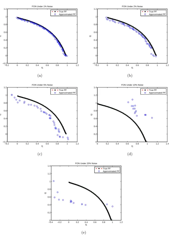
3.2 The evolved Pareto front of FON under the influence of noise levels (a)1%, (b)2%, (c)5%, (d)10% and (e)20% by MOEA/D. . . 53
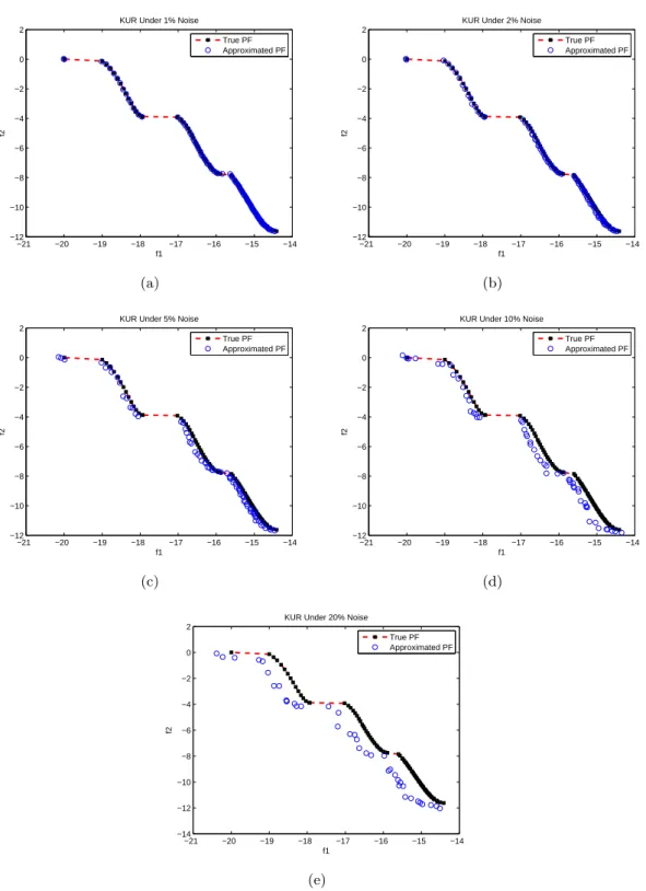
3.3 The evolved Pareto front of KUR under the influence of noise levels (a)1%, (b)2%, (c)5%, (d)10% and (e)20% by MOEA/D. . . 54
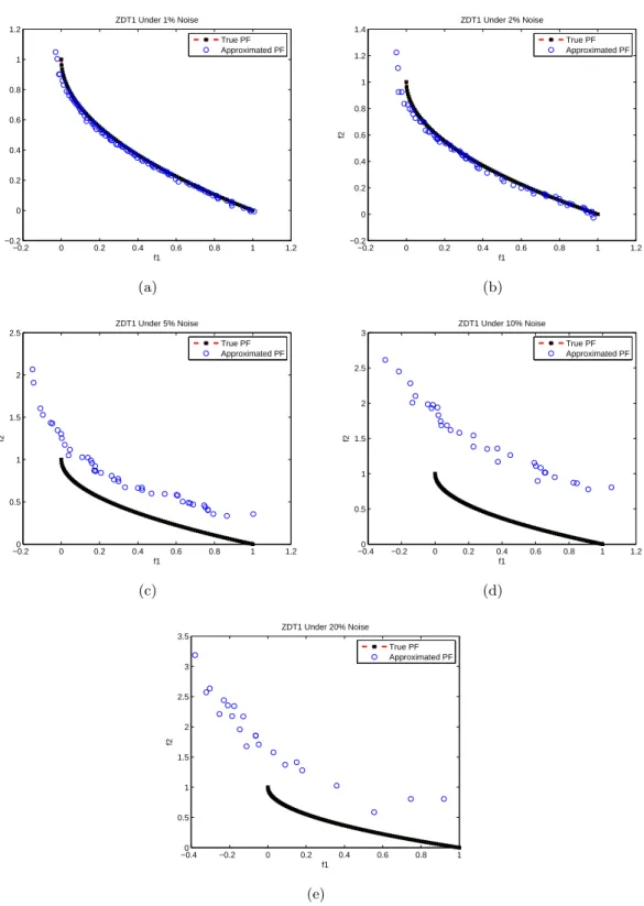
3.4 The evolved Pareto front of ZDT1 under the influence of noise levels (a)1%, (b)2%, (c)5%, (d)10% and (e)20% by MOEA/D. . . 55
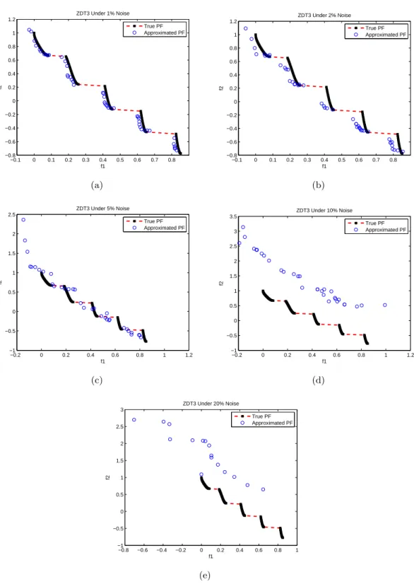
3.5 The evolved Pareto front of ZDT3 under the influence of noise levels (a)1%, (b)2%, (c)5%, (d)10% and (e)20% by MOEA/D. . . 56
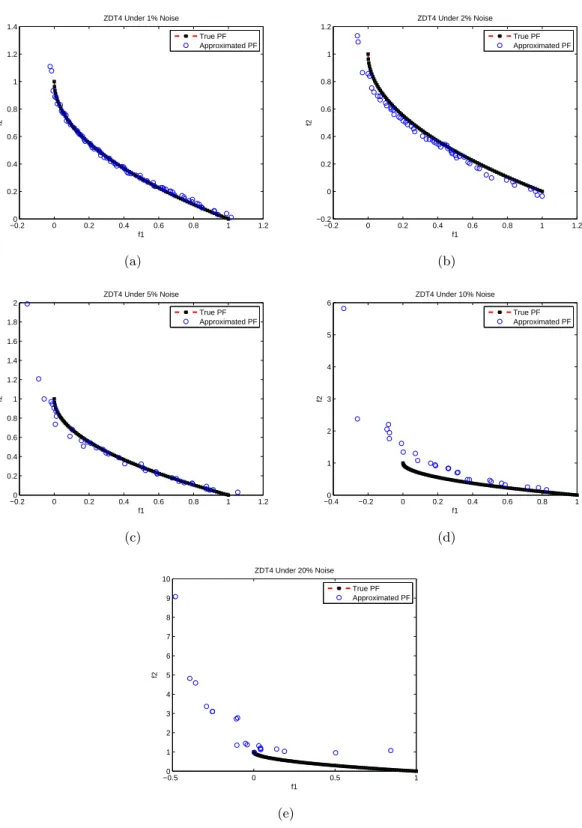
3.6 The evolved Pareto front of ZDT4 under the influence of noise levels (a)1%, (b)2%, (c)5%, (d)10% and (e)20% by MOEA/D. . . 57
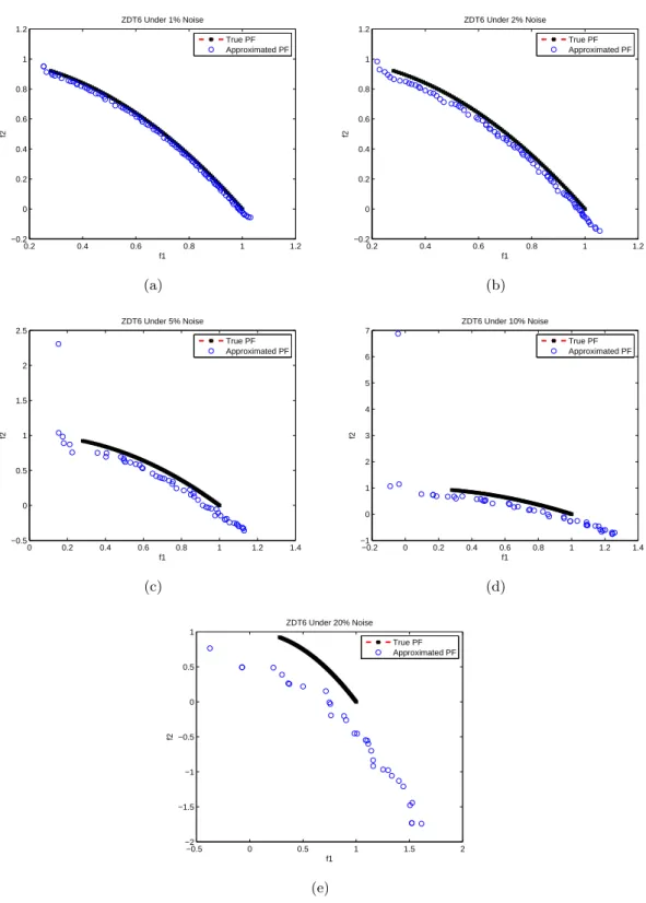
3.7 The evolved Pareto front of ZDT6 under the influence of noise levels (a)1%, (b)2%, (c)5%, (d)10% and (e)20% by MOEA/D. . . 58
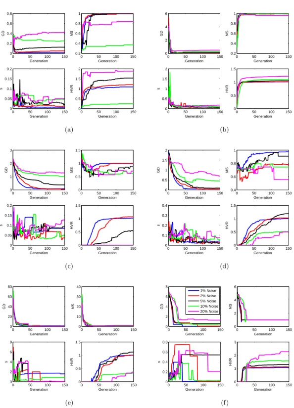
3.8 MOEA/D’s trace of performance metrics for (a) FON, (b) KUR, (c) ZDT1, (d) ZDT3, (e) ZDT4, (f) ZDT6. . . 59
4.1 Performance Metrics of MOEA/D+OO in presence of different noise lev-els for noisy FON problem. . . 69
4.2 Performance Metrics of MOEA/D+OO in presence of different noise lev-els for noisy KUR problem. . . 70
4.3 Performance Metrics of MOEA/D+OO in presence of different noise lev-els for noisy ZDT1 problem. . . 71
4.4 Performance Metrics of MOEA/D+OO in presence of different noise lev-els for noisy ZDT3 problem. . . 72
4.5 Performance Metrics of MOEA/D+OO in presence of different noise lev-els for noisy ZDT4 problem. . . 73
4.6 Performance Metrics of MOEA/D+OO in presence of different noise lev-els for noisy ZDT6 problem. . . 74
4.7 Pareto Front of noisy FON under the influence of noise level at (a)1%, (b)2%, (c)5%, (d)10%, (e)20% by MOEA/D+OO. . . 75 4.8 Pareto Front of noisy KUR under the influence of noise level at (a)1%,
(b)2%, (c)5%, (d)10%, (e)20% by MOEA/D+OO. . . 76 4.9 Pareto Front of noisy ZDT1 under the influence of noise level at (a)1%,
(b)2%, (c)5%, (d)10%, (e)20% by MOEA/D+OO. . . 77 4.10 Pareto Front of noisy ZDT3 under the influence of noise level at (a)1%,
(b)2%, (c)5%, (d)10%, (e)20% by MOEA/D+OO. . . 78 4.11 Pareto Front of noisy ZDT4 under the influence of noise level at (a)1%,
(b)2%, (c)5%, (d)10%, (e)20% by MOEA/D+OO. . . 79 4.12 Pareto Front of noisy ZDT6 under the influence of noise level at (a)1%,
(b)2%, (c)5%, (d)10%, (e)20% by MOEA/D+OO. . . 80 4.13 Performance metric of (a) GD, (b) MS, (c) S and (d) HVR for FON with
1% noise . . . 81 4.14 Performance metric of (a) GD, (b) MS, (c) S and (d) HVR for FON with
2% noise . . . 81 4.15 Performance metric of (a) GD, (b) MS, (c) S and (d) HVR for FON with
5% noise . . . 81 4.16 Performance metric of (a) GD, (b) MS, (c) S and (d) HVR for FON
with10% noise . . . 81 4.17 Performance metric of (a) GD, (b) MS, (c) S and (d) HVR for FON with
20% noise . . . 82 4.18 Performance metric of (a) GD, (b) MS, (c) S and (d) HVR for KUR with
1% noise . . . 82 4.19 Performance metric of (a) GD, (b) MS, (c) S and (d) HVR for KUR with
2% noise . . . 82 4.20 Performance metric of (a) GD, (b) MS, (c) S and (d) HVR for KUR with
5% noise . . . 82 4.21 Performance metric of (a) GD, (b) MS, (c) S and (d) HVR for KUR
with10% noise . . . 83 4.22 Performance metric of (a) GD, (b) MS, (c) S and (d) HVR for KUR with
20% noise . . . 83 4.23 Performance metric of (a) GD, (b) MS, (c) S and (d) HVR for ZDT1
with 1% noise . . . 83 4.24 Performance metric of (a) GD, (b) MS, (c) S and (d) HVR for ZDT1
with 2% noise . . . 83 4.25 Performance metric of (a) GD, (b) MS, (c) S and (d) HVR for ZDT1
with 5% noise . . . 84 4.26 Performance metric of (a) GD, (b) MS, (c) S and (d) HVR for ZDT1
with10% noise . . . 84 4.27 Performance metric of (a) GD, (b) MS, (c) S and (d) HVR for ZDT1
with 20% noise . . . 84 4.28 Performance metric of (a) GD, (b) MS, (c) S and (d) HVR for ZDT3
with 1% noise . . . 84 4.29 Performance metric of (a) GD, (b) MS, (c) S and (d) HVR for ZDT3
4.34 Performance metric of (a) GD, (b) MS, (c) S and (d) HVR for ZDT4
with 2% noise . . . 86
4.35 Performance metric of (a) GD, (b) MS, (c) S and (d) HVR for ZDT4 with 5% noise . . . 86
4.36 Performance metric of (a) GD, (b) MS, (c) S and (d) HVR for ZDT4 with10% noise . . . 86
4.37 Performance metric of (a) GD, (b) MS, (c) S and (d) HVR for ZDT4 with 20% noise . . . 87
4.38 Performance metric of (a) GD, (b) MS, (c) S and (d) HVR for ZDT6 with 1% noise . . . 87
4.39 Performance metric of (a) GD, (b) MS, (c) S and (d) HVR for ZDT6 with 2% noise . . . 87
4.40 Performance metric of (a) GD, (b) MS, (c) S and (d) HVR for ZDT6 with 5% noise . . . 87
4.41 Performance metric of (a) GD, (b) MS, (c) S and (d) HVR for ZDT6 with10% noise . . . 88
4.42 Performance metric of (a) GD, (b) MS, (c) S and (d) HVR for ZDT6 with 20% noise . . . 88
5.1 MOEA/D results for portfolio optimization problem with 60 assets (a) without noise, (b) 1%, (c) 2%, (d) 5%, (e) 10%, (f) 20%. . . 100
5.2 MOEA/D results for portfolio optimization problem with 60 assets (a) without noise, (b) 1%, (c) 2%, (d) 5%, (e) 10%, (f) 20%. . . 101
5.3 MOEA/D+OO results for portfolio optimization problem with 30 assets (a) without noise, (b) 1%, (c) 2%, (d) 5%, (e) 10%, (f) 20%. . . 102
5.4 MOEA/D+OO results for portfolio optimization problem with 30 assets (a) without noise, (b) 1%, (c) 2%, (d) 5%, (e) 10%, (f) 20%. . . 103
5.5 Algorithm A is better than B . . . 104
5.6 MOEA/D+OO vs. MOEA/D with respect to mean, standard divination and range of return for noisy portfolio optimization problem . . . 106
A.1 True Pareto front of ZDT1. . . 129
A.2 True Pareto front of ZDT3. . . 129
A.3 True Pareto front of ZDT4. . . 130
2.1 Create subproblems with evenly distributed weight vectors . . . 25 3.1 Definition of the test functions. . . 48 3.2 Performance metric values of estimated Pareto front by MOEA/D for
noisy FON . . . 51 3.3 Performance metric values of estimated Pareto front by MOEA/D for
noisy KUR . . . 52 3.4 Performance metric values of estimated Pareto front by MOEA/D for
noisy ZDT1 . . . 52 3.5 Performance metric values of estimated Pareto front by MOEA/D for
noisy ZDT3 . . . 52 3.6 Performance metric values of estimated Pareto front by MOEA/D for
noisy ZDT4 . . . 52 3.7 Performance metric values of estimated Pareto front by MOEA/D for
noisy ZDT6 . . . 52 4.1 Performance metrics values of estimated Pareto front by MOEA/D+OO
for noisy FON . . . 67 4.2 Performance metrics values of estimated Pareto front by MOEA/D+OO
for noisy KUR . . . 68 4.3 Performance metrics values of estimated Pareto front by MOEA/D+OO
for noisy ZDT1 . . . 68 4.4 Performance metrics values of estimated Pareto front by MOEA/D+OO
for noisy ZDT3 . . . 68 4.5 Performance metrics values of estimated Pareto front by MOEA/D+OO
for noisy ZDT4 . . . 68 4.6 Performance metrics values of estimated Pareto front by MOEA/D+OO
for noisy ZDT6 . . . 68 5.1 Result of portfolio optimization returns with 30 assets by MOEA/D . . 99 5.2 Result of portfolio optimization returns with 60 assets by MOEA/D . . 99 5.3 Result of portfolio optimization returns with 30 assets by MOEA/D+OO 104 5.4 Result of portfolio optimization returns with 60 assets by MOEA/D+OO 104
MOEA Multi-objective Optimization Evolutionary Algorithm SPEA Strength Pareto Evolutionary Algorithm
NSGA-II Non-dominated Sorting Genetic Algorithm-II ELDP Experimental Learning Directed Perturbation GASS Gene Adaptation Selection Strategy
MOEA/D Multi-objective Optimization Evolutionary Algorithm based on Decompo-sition
MOP Multi-objective Optimization Problem OO Ordinal Optimization
MOEA/D+OO Combined MOEA/D algorithm with OO technique VOO Vector Ordinal Optimization
SVR Support Vector Regression ANN Artificial Neural Network PF Pareto Front
PS Pareto-optimal Set
NTSPEA Noise Tolerant Version of SPEA
MOEA-RF Robust Feature Multi-objective Evolutionary Algorithm MNSGA-II Modified Non-dominated Sorting Genetic Algorithm-II MOPSEA Multi-objective Probabilistic Selection Evolutionary Algorithm SOP Single-objective Optimization Problem
DMOEA-DD Dynamical Multi-Objective Evolutionary Algorithm with Domain De-composition
OGA Order Based Genetic Algorithm GOO Genetic Ordinal Optimization
OCBA Optimal Computing Budget Allocation
CPSOO Combined Particle Swarm with Ordinal Optimization xiii
• Chapter 4: MOEA/D With Ordinal Optimization Technique for Handling Noisy Problems.
1. Hamid R. Jalalian, Qingfu Zhang and Edward Tsang, “Combining MOEA/D with Ordinal Optimization for Noise Handling Purpose”, to be submitted to journal of “Computational Intelligence”.
• Chapter 5: Noisy Portfolio Optimization Problem.
1. Hamid R. Jalalian and Edward Tsang, “An Investigation on Noisy Portfolio Optimization Problem”, to be submitted to journal of “Intelligent Systems in Accounting, Finance and Management”.
Many real life applications involve multiple (potentially conflicting) objective functions that must be optimized simultaneously. In the case of conflicting objectives, no single solution can be optimal to all objectives. Thus, a strong and powerful optimization algorithm is required to be capable of finding a set of solutions that will represent the best tradeoffs amongst the all objectives. This set of solutions is known as the Pareto optimal solution.
Evolutionary algorithms fall within a class of stochastic search methods that are capable of estimating Pareto optimal solutions in a single run. They are able to do this because the algorithms update their population of solutions at each generation. As a result, this method is proving itself to be very effective at solving complicated multi-objective optimization problems.
Finding a good Pareto-optimal estimation is not the only challenge facing the
mization algorithm, however. Uncertainty is also a disruptive phenomenon that char-acterizes many real world optimization problems in various forms. In recent decades numerous studies [4–6] have been conducted into different types of uncertainty and these are listed in the next section.
1.1
Sources of Uncertainty
• Uncertainty of environment: for example, temperature, moisture, perturbation in speed or dynamic fitness function.
• Uncertainty of optimization parameters: for instance, parameters of a solution subject to change or perturbation after implementation, but still required to func-tion for manufacturing tolerance. This type of uncertainty is known as a search for robust solution.
• Uncertainty introduced due to unavailability of original fitness function or where the analytical fitness function is computationally very expensive. In this instance, the solution must be approximated.
The work presented in this thesis addresses this third version of uncertainty, also known as the optimization of noisy problems.
1.2
Thesis Motivation
A very important and also very sensitive research area is the study of noise, and the ways to cope with it, in the evolutionary multi-objective optimization algorithm. There are a number of studies that suggest different strategies or noise handling techniques for tackling disruptive noise by very well known MOEA. For instance,
• Strength Pareto Evolutionary Algorithm (SPEA) introduced by Zitzler in 1999 [7]. A Noise Tolerant Version of SPEA (NTSPEA) by Buche [8]. Zitzler and Buche proposed three modifications for handling noise for this particular dominance based MOEA, namely i) Domination dependent lifetime, which defines a lifetime
• A Robust Feature Multi-objective Evolutionary Algorithm (MOEA-RF). Goh and Tan proposed three noise handling techniques and incorporated them into a simple MOEA, naming the new algorithm MOEA-RF. The three noise handling features are the Experimental Learning Directed Perturbation (ELDP), the Gene Adaptation Selection Strategy (GASS) and a possibilistic archiving methodology [9].
• A Modified Non-dominated Sorting Genetic Algorithm-II (MNSGA-II). Deb in-troduced the Non-dominated Sorting Genetic Algorithm-II (NSGA-II) and Babbar introduced a modification of its ranking scheme to handle noise. The new scheme allows the algorithm to expand its Rank 1 frontier by adding close neighbour-ing solutions to the rank. It also incorporates a procedure to keep only reliable solutions in the final non-dominated solution set. [10].
MOEA/D, which is a very well established decomposition-based MOEA, introduced for the first time by Zhang and Li in 2007 [11], will be utilised in this thesis to confront noise problems.
As with the other algorithms detailed in Section 1.2, this thesis will investigate MOEA/D in a noisy environment. In order to reach our stated goal certain steps must be taken, the first of which being an answer to the following questions.
• How effective is MOEA/D in the presence of noise?
It is important to analyse the performance of MOEA/D in the presence of different levels of noise, from low to medium to high. Will its performance deteriorate with increased noise? if so, by how much? In order to measure these qualities, different performance metrics will be implemented (see section 3.4).
• What technique best assists MOEA/D to handle noise?
Due to the fact that most of the studies on noisy environments explore MOEAs that are based on dominance their noise-handling methods will not be useful for MOEA/D, which is a decomposition-based algorithm. Furthermore, their results are not comparable because parameter settings have a bearing on different algo-rithms’ performance. Thus, in this work, we are seeking a novel technique for handling noise in conjunction with the basic MOEA/D. Our technique will ideally cope with noisy problems and estimate more reliable solutions for them.
Finally, we will assess the new algorithm as to its suitability for real life application.
1.3
Thesis Contribution
As previously mentioned, this work will study MOEA/D in the presence of different levels of noise. The major contributions of this thesis are listed as follows:
1. This is the first piece of research that studies the effect of noise on the performance of MOEA/D.
2. We will prove that the performance of MOEA/D deteriorates as noise levels in-tensify.
3. In Chapter 4 a new algorithm, MOEA/D+OO, based on the MOEA/D framework will be introduced. This is a modified version of MOEA/D that is significantly better suited to handling noise.
4. We will prove that MOEA/D+OO significantly outperforms MOEA/D in the noisy multi-objective optimization problem.
5. We study noisy portfolio optimization for the first time by adding noise only to the return values of the objective function.
6. In this thesis, the noisy portfolio optimization problem is used as a real world application to test the algorithms’ performance.
1.4
Thesis Outline
The organization of this thesis is as follows:
Chapter 2 provides a review of multi-objective evolutionary algorithms. In this chapter, the fundamentals of evolutionary algorithms and MOP will be summarized. Chapter 3 assesses the performance of MOEA/D in a noisy environment. This chapter explains the theory and methodologies that have been used to examine and assess the algorithm. Chapter 4 proposes a noise handling technique to handle noisy problems. A new algorithm is developed that combines Ordinal Optimization (OO) with MOEA/D. Chapter 5 details the introduction of the algorithm into a real life problem: a classical finance problem in a noisy environment. Finally Chapter 6 presents conclusions, which will wrap up this thesis and propose possible future works.
2
Background and Literature Review
This chapter will briefly discuss the principals of optimization theory and the different types of optimization problem. A literature review of previous research studies into multi-objective optimization problems is delivered, along with a discussion of the tradi-tional methods and evolutionary algorithms used for solving multi-objective problems. Thereafter, the major issues in multi-objective optimization evolutionary algorithms (MOEAs) are discussed, alongside a classification of the different MOEAs.
The base algorithm used in this thesis is MOEA/D. A detailed review of it has been prepared in Section 2.4, followed by a look at the literature on noisy MOEAs.
In conclusion, this chapter details the principals of ordinal optimization theory (OO) that are going to be used for noise handling in this study to assist MOEA/D in solving noisy multi-objective problems.
specific constraints of their area.
In this section, a succinct general summary and classification of the optimization problem is provided, alongside a look at other issues in this area such as different optima types or different problems.
2.1.1 Elements of an Optimization Problem
There are three major elements which are common to any optimization problem as follows [12]:
• An objective function. A system model, representing the quantity to be opti-mized.
• A set of variables. These impact the value of the objective function.
• A set of constraints. These restrict the values that can be assigned to the variables.
The goal of any optimization method is to assign values, from a given domain, to the variables of the objective function to be optimized such that all constraints are satisfied. In this research, the search space is denoted by Ω . In the case of a constraint problem, a solution is found in the feasible space that is denoted byF. Always,F ⊆Ω .
2.1.2 Classification of Optimization Methods
The different classifications are made according to the specific characteristics of the methods used. For instance, optimization methods can be divided into two major classes [12], dictated by the solutions found, as follows.
• Local search algorithm: information local to the current solution is used to produce a new solution.
• Global search algorithm: the entire domain is searched for optima. Further classifications can be introduced as follows:
• Stochastic: this method uses random elements to transform a candidate solution into a new solution.
• Deterministic: in which no random elements are applied.
2.1.3 Classification of Optimization Problems
Optimization problems can have many characteristics and classifications of these can be proposed according to the following [12]:
• Number of variables: single variable to multi-variable.
• Type of variable: continuous or discrete.
• Degree of non-linearity: linear, quadratic, etc.
• Type of constraint: boundary, equality and/or inequality.
• Number of optima: optimization problems can have one (unimodal) or many (multimodal) solutions.
• Number of optimization criteria: if only one objective function requires op-timization, it is a ‘Single Objective Problem’. If more than one objective function must be optimised simultaneously, the problem becomes ‘Multi-objective’.
2.1.4 Multi-objective Optimization Problems
Most real-world search and optimization problems naturally involve multiple objectives. The extremist principle mentioned above cannot only be applied to one objective when the rest of the objectives are just as important. Different solutions may produce tradeoffs
straints. Objective functions and constraints are functions of the decision variables. The optimization goal is to min y=F(x) = (f1(x), f2(x), ..., fm(x)) s.t C(x) = (c1(x), c2(x), ..., cr(x))≤0 x= (x1, x2, ..., xn)∈Ω x(iL)≤xi≤x (U) i f or i= 1,2, ..., n y= (y1, y2, ..., ym)∈Λ (2.1)
where x is the decision vector, y is the objective vector, Ω is denoted as the decision space, andΛ is the objective space. Mapping between the solution space and the objective space is illustrated in Figure 2.1. The constraints C(x)≤0 determine the set of feasible solutions [2].
The solutions x∈Ω of continuous MOPs are a vector of nreal variables. Neverthe-less the solutions of discrete MOPs are vectors of ninteger variables.
The definition of optimality is not straightforward, due to totally conflicting, non-conflicting or partially non-conflicting objective functions. It is therefore necessary to outline the specific definition of ‘optimum’ for the MOP: for an MOP the optimum means a balance point between all of the objectives. In other words, improving any one objective may bring about the degrading of other objectives. Thus, our task is to find solutions that balance these tradeoffs. A significant number of solutions may exist for our MOP, so in order to tackle this task, it is necessary to put forward a set of definitions.
Most multi-objective optimization algorithms use the concept of dominance in their search.
Definition 2 (Dominance) A solution x1 is said to dominate another solution x2 ,
if both conditions 1 and 2 are true:
1. The solution x1 is no worse than x2 in all objectives, or fi(x1) ≤ fi(x2) for all i= 1,2, ..., m.
2. The solution x1 is strictly better than x2 in at least one objective, or fj(x1) < fj(x2) for at least one j∈ {1,2,· · ·m}.
If either of the above conditions is violated, the solution x1 does not dominate solutionx2. Ifx1does dominate solutionx2(or mathematicallyx1x2), it is customary to note any of the following [13]:
• x2 is dominated byx1 • x1 is non-dominated by x2 • x1 is non-inferior tox2.
Definition 3 (Pareto Optimal Set) For a given MOP 2.1, the Pareto Optimal Set (see Figure 2.2), P∗, is defined as:
P∗:={x∈Ω | @ x0 ∈Ω F(x0)F(x)}. (2.2) The Pareto-optimal Set (PS) contains all balanced tradeoffs which represent the MOP solutions.
The Pareto front contains all the objective vectors corresponding to the decision vectors that are not dominated by any other decision vector (see Figure 2.2).
Figure 2.2: Illustration of Pareto front and Pareto set [2].
It is appropriate to note the characteristics of a Pareto front:
1. The Pareto front contains the Pareto-optimal solution and, in the case of a con-tinuous front, divides the objective function space into two parts: non-optimal solutions and infeasible solutions.
2. A Pareto front is not necessarily continuous.
3. The Pareto front can be concave, convex, or a combination of either.
5. The Pareto front may continue towards infinity, even in the case of boundary constrained decision variables.
6. Due to mapping, neighbouring points in a Pareto front (objective function space) are not necessarily neighbours in the decision variable space.
2.1.4.1 Ideal and Nadir Points (Objective Vectors)
We assume that the objective functions are bounded over a feasible region, with two special objective vectors ideal and nadir point to define the lower and upper bounds of PF. Figure 2.3 illustrates both points in the objective space of a hypothetical two objective minimization problem. Definitions of both points are given below.
Definition 5 (Ideal point) A pointzidl={z1,· · · , zm}in the objective space is called an ideal point if it has the best value for each objective: ziidl= min
x∈Ωfi(x) ∀ i={1, ..., m}
for problem 2.1.
Definition 6 (Nadir point) A point znad = {z1,· · · , zm} in the objective space is called a nadir point if it has the worst value for each objective: zinad= max
x∈Ω fi(x) ∀ i= {1, ..., m} for problem 2.1.
Figure 2.3: Illustration of Nadir and Ideal points [1].
2.1.5 Classification of an MOP
Multi-objective optimization problems have been around for at least the last four decades and many algorithms have been evolved to solve them. Researchers have at-tempted to classify these algorithms according to various considerations. Cohon [14] classified them into the following two types:
and Masud [15] and later Miettinen [1] fine-tuned the above classification and suggested the following four classes:
• No-preference methods.
• A posteriori methods.
• A priori methods.
• Interactive methods.
The no-preference methods assume no information about the importance of objec-tives, but a heuristic is used to find a single optimal solution. It is important to note that although no preference information is used, these methods do not make any at-tempt to find multiple Pareto-optimal solutions. Posteriori methods do use preference information on each objective and iteratively generate a set of Pareto-optimal solutions. The classical method of generating Pareto optimal solutions requires some knowledge of the algorithmic parameters that will guarantee the finding of a Pareto-optimal solution. On the other hand, A priori methods use more information about the preferences of objectives and usually find one preferred Pareto-optimal solution. Interactive meth-ods use the preference information progressively during the optimization process as the decision-maker interacts with the optimization program during the optimization process. Typically the system provides an updated set of solutions and lets the decision-maker consider whether or not to change the weighting of individual objective functions.
The popularity of using a weighted sum of objective functions is obvious: it is trivial to implement and it effectively converts a multi-objective problem into a single objective one. A known drawback is that in the case of a high number of objective
functions, the appropriate weighting is painful to choose a priori by the decision-maker. Furthermore, scaling of the individual objective function values is often required due to different function value ranges. With regard to the popularity of a posteriori techniques, especially Pareto-optimization techniques, there are two obvious candidate explanations:
1. The decision-makers are willing to perform unbiased searches.
2. The decision-makers are unwilling or unable to assign priorities without having further information about the other potential/effective solutions.
2.2
Traditional Methods of Solving MOPs
Classical ways to address this problem used direct or gradient based methods that rendered them insufficient or computationally expensive for large scale or combinatorial problems. Other difficulties attended the classical methods, such as problem knowledge, which may not be available, or sensitivity to some problem features. For example, finding solutions on the entire Pareto optimal set can only be guaranteed for convex problems. Classical methods for generating the Pareto front set aggregate the objectives into a single or parametrized function before search. Thus, several runs and parameter settings are performed to achieve a set of solutions that approximate the Pareto optimal.
2.2.1 The Weighted Sum Method
The idea behind this method is to associate each objective function with a weighting coefficient and minimize the weighted sum of the objective. In this way, multiple ob-jective functions are transformed into a single obob-jective function. More accurately, the multi-objective optimization problem is modified into the following problem, known as a weighted problem: minimize m X i=1 wifi(x) s.t x∈Ω (2.4)
Theorem 3 Let the multi-objective optimization problem be convex ifx∗ is Pareto op-timal, then there exists a weighting vector w (wi ≥ 0 , i= {1, ..., m} , Pki=1wi = 1.) such that x∗ is a solution of the weighted problem (2.4).
For the proof of all theorems, refer to [1].
Theorem 1 to 3 state the solution of the weighting method is Pareto optimal if the weight coefficients are all positive [1]. The disadvantage of this method is that it is limited solely to convex problems, because a whole solution cannot be found for non-convex problems.
2.2.2 ε-Constraint Method
In the ε-constraint method one of the objective functions is selected to be optimized and all the other objective functions are converted into constraints by setting an upper bound to each of them. The problem to be solved is now of the following form
minimize fl(x)
s.t fi(x)≤εi, ∀ i= 1, ..., m , i6=l
s.t x∈Ω
(2.5)
wherel∈ {1, ..., m}. Problem (2.5) is called an ε−constraint problem.
Theorem 4 The solution ofε−constraint problem (2.5) is weakly Pareto optimal.
Theorem 4 states that the solutions of equation 2.5 are weakly Pareto optimal with-out any additional assumptions. After this the theorem 5 regarding the proper Pareto optimality of the solutions of theε−constraintproblem can be introduced as follows, Theorem 5 A decision vector x∗ ∈Ω is Pareto optimal if and only if it is a solution of ε-constraint problem (2.5) for every l = 1, ..., m, where εi = fi(x∗) f or i = 1, ..., m, i6=l.
Proof in [1].
2.2.3 Value Function Method
In this method, the decision maker must be able to give an accurate and explicit math-ematical form of the value function U :Rm →R that represents his or her preferences
globally. This function provides a complete ordering in the objective space.
maximize U(f(x))
s.t x∈Ω
(2.6)
The value function problem is then ready to be solved by any single objective optimization method.
Theorem 6 Let the value function U : Rm → R be strongly decreasing. Let U attain
its maximum atf∗. Then, f∗ is Pareto optimal. Proof in [1].
2.3
Multi-objective Evolutionary Algorithm
2.3.1 Evolutionary Algorithm
Evolution is an optimization process that improves the ability of a system to survive in competitive environments [12]. Inspired by Charles Darwin’s theory of ‘natural
se-• Small changes in the location (decision variables) of the offspring ⇐⇒Mutation. The evolutionary algorithm (EA) is a stochastic optimization method. The earliest study in this field dates back to the 1950s and, since the 1970s, several evolutionary methodologies have been proposed. All of these approaches operate on a set of candi-date solutions. Using strong simplifications, this set is subsequently modified by two basic principles: selection and variation. While ‘selection’ mimics the natural world’s competition for reproduction and resources among living beings, the other principle, variation, imitates the natural ability to create new beings by means of recombination and mutation.
Evolutionary algorithms such as evolution strategies and genetic algorithms are of-ten used for solving optimization problems that are too complex to be solved using traditional mathematical programming methods [12]. EAs require little knowledge of the problem to be solved and are easy to implement, robust, and inherently parallel.
2.3.2 Multi-objective Optimization Problems using EAs
To solve an optimization problem by EA, one must be able to evaluate the objective (cost/loss) functions for a given set of input variables. Due to their ease of implementa-tion, and fitness for parallel computing, EAs are eminently suited to complex problems. Most real-world problems involve simultaneous optimization of several often conflicting objectives. Multi-objective EAs are able to find a set of optimal trade-offs in a single run [2, 13].
EAs work with ‘individuals’ in a population. The number of individuals in the population is called ‘popsize’ and each individual has two properties:
• Quality, known as ‘fitness value’.
After obtaining the fitness values of all individuals, the selection process generates a ‘mating pool’. Only individuals with higher fitness values are allowed into the mating pool. Selected individuals are called ‘parents’.
Then, two parents might be selected randomly from the mating pool to generate two ‘offspring’. After which, the newly generated individuals replace the old ‘parents’ and another generation starts.
2.3.3 Major Issues in MOEAs
MOEAs regulate the following processes in order to achieve a good approximation of a Pareto front.
2.3.3.1 Reproduction Operators
Reproduction is the process of producing offspring from selected parents. Thus an operator needs to combine or change the value of the parents in the decision space to create new individuals.
The operator that combines the genome of the parents to produce a new individual is called the ‘Crossover’. ‘Mutation’ changes the value of genes in a chromosome ran-domly. From the first evolutionary algorithm introduced to the current day, different reproduction operators have been proposed, including:
(i) Binary reproduction operators such as, one point, two point or uniform crossover and Gaussian or uniform mutation [2, 13].
(ii) Floating point operators such as, simulated binary crossover (SBX) [16], uni-modal normal distribution operator (UNDX) [17], deferential evolution (DE) [18] and simplex crossover (SPX) [19] or polynomial mutation [13] and Gaussian mutation oper-ator [20]. The floating point operoper-ator shows better performance when decision variables are floating point values (Real numbers).
with the decision variables from another predetermined vector to create a trial vector. Parameter mixing is often referred to as ‘crossover’. There are two predetermined parameters, differential weight (F ∈[0,2]) and crossover probability (CR∈[0,1]), that need to be set up either by practice or through a specific method, for instance rules of thumb for selecting parameters [18]. The basic DE algorithm is described in Algorithm 2.1.
Algorithm 2.1 DE
Input: 1) Three randomly selected individuals x1, x2, x3 = (x1, x2, ...xn). 2) F differential weight.
3) CR crossover probability
Output: New individual x0 = (x01, x02, ..., x0n).
Step 1) Create vectorU with uniformly distributed numberU = (u1, u2, ..., un) Step 2) ifui < CRthenx0i =xi1+F×(x3i −x2i)
Step 3) otherwise setx0i =x1i fori= 1,2, ..., n.
Sometimes, the newly created candidate falls out of the bounds of the decision variable space. We address this problem by simply replacing the candidate value that violated the boundary constraints with the closest boundary value [21].
2.3.3.1.2 Gaussian Mutation If the uniformly distributed number u ∼ U(0,1) is greater than the mutation probability (Pmu) then this operator adds a Gaussian distributed random value to the decision variables of the chosen individual. If it falls out of the boundary of the decision variables then the violating values are replaced with the closest boundary value [22, 23]. The Gaussian density function is
fG(0,σ2)(x) = 1 √ 2πσ2e −x2 2σ2
2.3.3.2 Fitness Assignment
As only the best performing individuals get the chance to reproduce, it is important to generate a function that will determine the fitness of each individual, known as ‘Fitness Function’. A fitness function maps a fitness vector to a single value, which represents the quality or rank of the individual in the population. Moreover, the fitness function guides the MOEA to search into promising areas in the search space. Pareto dominance ranking, indicator-based and decomposition-based rankings are three major fitness assignment strategies used in MOEAs.
2.3.3.3 Convergence
It is important for any optimization framework to find actual solutions to optimization problems or to make a good estimation of a solution. This process is called convergence. As with any optimization technique, converging to the true Pareto front is important for all MOEAs. Algorithms are comparative in their converging speed [24, 25].
2.3.3.4 Diversity
Obtaining a good distribution of generated solutions along the Pareto front is called ‘Diversity’. A diversity maintenance technique avoids convergence of a population to a single solution. Therefore, it is very important. It is a fact that an even spread of discovered solutions is more desirable and different techniques have been established to preserve the diversity of solutions along the Pareto front such as, niche sharing [26], clustering [27], crowding density estimation [28], and nearest neighbour method [29].
2.3.3.5 Elitism
The process that guarantees survival of the best individual in the current population to the next generation is called ‘Elitism’. To ensure this, a copy of the current population will be kept, without being mutated; in other words, elitism in MOEAs makes sure that the best (or elite) solutions are kept in a safe place between generations.
In this study we classify the MOEA according to their fitness assignment methods and divide these into three categories including:
2.3.4.1 MOEAs based on Pareto Dominance
One of the most popular approaches to fitness assignment appears to be the Pareto-based ranking. Since its inception, Pareto-based MOEAs such as MOGA [30], PAES [31], NSGA-II [32], SPEA-II [33] have emerged as the most widely used. However, both Fonseca and Fleming [34], [30] have highlighted the inadequacy of an MOEA based on Pareto assignment in high dimensional objectives. In this situation, the Pareto-based MOEA may not be able to produce sufficient selection pressure and also its performance does not scale well with respect to the number of objectives [35].
2.3.4.2 MOEAs Based on Decomposition
This approach aggregates the objectives into a single scalar to approximate the Pareto front. It was in fact the failure of Pareto-based MOEAs in the high dimensional ob-jective space that turned attention to decomposition-based methods. MOGLS [36] and MOEA/D [11] are the two most successful algorithms in this category.
2.3.4.3 MOEAs Based on Indication
Here, the fitness function seeks to rank population members according to their perfor-mance in relation to the optimization goal. MOEAs then introduce a utility function to be maximized. For example, one possibility would be to sum up the indicator val-ues for each population member with respect to the rest of the population [37], [38]. IBEA, which was introduced by Zitzler and K¨unzli, is an example of an indicator-based evolutionary algorithm. For more information see [37].
The Non-dominated Sorting Genetic Algorithm, NSGA-II, is undoubtedly the most well-known and referenced algorithm in the multi-objective literature. It is a GA with random mating of individuals within a population. It is based on obtaining a new population from the original one by applying the typical genetic operators (selection, crossover and mutation); then, the individuals in the two populations are sorted ac-cording to their rank, and the best solutions are chosen to create a new population. In the case of having to select some individuals with the same rank, a density estimation based on measuring the crowding distance to the surrounding individuals belonging to the same rank is used to get the most promising solutions [32]. In 2014 a new version of this algorithm was introduced based on adaptive updating and including new refer-ence points on the fly. The resulting adaptive NSGA-III is shown to provide a denser representation of the Pareto-optimal front [39, 40].
The Strength Pareto Evolutionary Algorithm, SPEA2, works on the same random mating of individuals within a population as NSGA-II. In this algorithm, each individual has a fitness value assigned, which is the sum of its strength raw fitness and a density estimation. The algorithm applies the selection, crossover, and mutation operators to fill an archive of individuals; then, the non-dominated individuals of both the original population and the archive are copied into a new population. If the number of non-dominated individuals is greater than the population size, a truncation operator, based on calculating the distances to the (k−th) nearest neighbour, is used [29].
2.4
MOEA/D as a Framework
In this thesis, MOEA/D has been studied for handling noisy MOP and this framework will be reviewed as follows:
In order to find a set ofN Pareto optimal solutions, MOEA/D decomposes an MOP toN Single-objective Optimization Problem (SOP) (see Figure 2.4). It then solves each subproblem independently. (See Figure 2.5).
Figure 2.4: Decomposing MOP to N Subproblems.
Figure 2.5: MOEA/D solve N subproblems simultaneously.
2.4.1 Decomposition Methods
Decomposition is a general approach to solving a problem by breaking it up into smaller ones and solving each of the smaller ones separately, either in parallel or sequentially. [41].
Decomposition in optimization is an old idea and appears in early work on large-scaleLP s[42]. The original primary motivation behind decomposition methods was to solve very large problems that were beyond the reach of standard techniques.
Decomposition of an MOP can be done at different levels. i) Decision variables: in [43] the authors introduced a Dynamical Multi-Objective Evolutionary Algorithm with Domain Decomposition (DMOEA-DD) by using a domain decomposition technique. The decomposition of decision variables is implemented by splitting the original set
of decision variables into subgroups and optimizing each group as a subproblem. ii) Objective functions: in [11, 44] the authors introduced algorithms that decompose an MOP into multiple scalar optimization subproblems.
In the following the Tchebycheff decomposition method is introduced. This will be used later in this thesis.
2.4.1.1 Tchebycheff Decomposition Method
The Tchebycheff approach was introduced in [45]. The aggregation function of this method is mathematically defined as follows,
minimize gte(x|λ, z∗) = max i∈1,···,mλi|fi(x)−z ∗ i| subject to x∈Ω⊂Rn. (2.7)
where z∗ = (z1∗,· · · , zm∗) is the reference point. zi∗ = min{fi(x) | x ∈Ω} for each
i= 1,· · · , m. The reference point guides the search procedure to converge. (see Figure 2.6).
According to the following theorem for any Pareto optimal solution x∗ there is a weight vector (λ1, λ2) such thatx∗ is the optimal solution to (2.7).
Theorem 7 If the Tchebycheff problem 2.7 has a unique solution, then it is Pareto-optimal.
Proof of this theorem is available in [1].
2.4.2 Subproblems
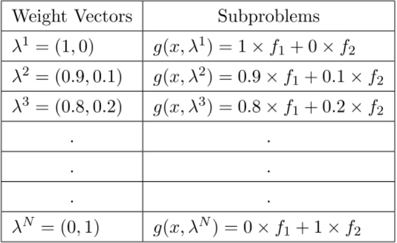
Generating a diverse set of weight vectors is intransitive for the decomposition of the multi-objective problem into multiple single objective problems in order to achieve a good representation of Pareto Front (PF). Table 2.1 shows the process of creating sub-problems based on an aggregation function. Every weight vector defines a subproblem and a diverse set of weight vectors leads to a diverse range of subproblems. This results in a diversity of Pareto optimal solutions because, as is mentioned in Section 2.4.1.1,
Figure 2.6: Tchebycheff Decomposition Method.
Table 2.1: Create subproblems with evenly distributed weight vectors
Weight Vectors
Subproblems
λ
1= (1
,
0)
g
(
x, λ
1) = 1
×
f
1+ 0
×
f
2λ
2= (0
.
9
,
0
.
1)
g
(
x, λ
2) = 0
.
9
×
f
1+ 0
.
1
×
f
2λ
3= (0
.
8
,
0
.
2)
g
(
x, λ
3) = 0
.
8
×
f
1+ 0
.
2
×
f
2.
.
.
.
.
.
λ
N= (0
,
1)
g
(
x, λ
N) = 0
×
f
1+ 1
×
f
2the optimal solution of 2.7 is a Pareto optimal solution for 2.1. This fact is clearly illus-trated in Figure 2.7. The authors in [11] introduced a method for generating uniform weight vectors.
2.4.3 Neighbourhood
Neighbourhood relation in MOEA/D is introduced by computing the Euclidean dis-tances between any two weight vectors and then working out the T closest weight vectors to each weight vector. T is the size of neighbourhood which is set by the deci-sion makers. For each i= 1,· · ·, N set B(i) ={i1,· · ·, iT} where λi1,· · · , λiT are the closest weight vectors to λi. Note that each weight vector is the closest vector to itself and the neighbourhoods of weight vectors remain unchanged during the whole search process. Figure (2.8) illustrates the neighbouring relations in MOEA/D. T is a major
Figure 2.8: Illustration of neighbouring relation in MOEA/D. (T is the size of neighbourhood)
control parameter in MOEA/D [11] because it is a mating restriction. Two solutions have a mating chance if they are in the same neighbourhood.
2.4.4 General Framework
In the framework of MOEA/D, a population of scalar optimization subproblems is maintained and each subproblem is formed by the following components:
• Solution x: is the current best solution of this subproblem.
• Weightλ: is the weight vector that characterizes this subproblem and determines its search direction.
• Neighbourhood B: the list for each subproblem that contains the indexes of neigh-bouring subproblems.
subproblems within the neighbourhood of subproblem i. If y is fitter than any neighbours, then y will replace that particular neighbour.
A stopping criteria is necessary to stop the algorithm from searching. In this thesis, the stopping criteria employed is a predetermined number of generations. An external population that holds the best solutions is not practical in continuous MOPs, however. This is because the final generation of this population represents the best result found by MOEA/D an inherent elitism that plays an important role in discrete MOPs. However, in our experiments we focus purely on continuous MOP and for this reason the next chapters will not employ the external population. Finally, the reference point is a vector which directs the algorithm towards the optimal solution. A reference point constructed asz∗ = (z1∗,· · ·, zm∗) where zi∗ = min {fi(x) | x ∈ Ω} for each i = 1,· · · , m. This can be updated during the search or can be fixed as a predetermined parameter. Algorithm 2.2 describes MOEA/D in detail and more information is available in [11].
In the less than a decade since Zhang and Li introduced MOEA/D in 2007 [11] it has attracted much interest and numerous research studies have been published on the following aspects [46]:
1. Combining MOEA/D with other meta-heuristics, such as simulated anneal-ing [47], colony optimization [48], particle swarm optimization [49, 50], tabu search [51], guided local search [52]and deferential evolution [53].
2. Changing the reproducing operators, such as guided mutation operator [54], nonlinear crossover and mutation operator [55], differential evolution schemes [53], and a new mating parent selection mechanism [46, 56].
3. Research on decomposition techniques. An NBI-style Tchebycheff decom-position approach is proposed to solve portfolio optimization problems by the authors in [57]. In [58, 59] different decomposition approaches are used simultaneously.
4. Improvement on weight vectors. Predetermined, uniformly distributed weight vectors are used to define scaler subproblems in MOEA/D. This reveals that the fixed weight vectors used in MOEA/D might not be able to cover the whole PF very well [47]. Therefore, in [60], the authors create weight vec-tors predictably based on the distribution of the current weight set. In [61], another weight adjustment method is developed by sampling the regression curve of the objective vectors of the solutions in an external population. The authors in [46] introduce (MOEA/D-AWA), which is an improved version of MOEA/D with an adaptive weight vector adjustment.
5. Applications of MOEA/D like the combinatorial optimization problem, known as the knapsack problem, [47, 58], the travelling salesman problem [47], the flow-shop scheduling problem [51,62] and the capacitated arc routing problem [63]. Or practical engineering problems like antenna array synthesis [64, 65], wireless sensor networks [66], robot path planning [67], missile control [68], a multi-objective optimization for rest-to-rest manoeuvres of flexible space-craft [69], portfolio management [57] and rule mining in machine learning [70] have also been investigated.
Input:
• A stopping criterion.
• N: the number of subproblems considered in MOEA/D.
• A uniform spread of the weight vectors: λ1,· · ·, λN.
• T: the number of weight vectors in the neighbourhood of each weight vector. Output:
• EP or {F(x1),· · ·, F(xN)}. Step 1) Initialization:
Step 1.1) Set EP =∅.
Step 1.2) Compute the Euclidean distances between any two weight vectors. For each subproblemi= 1, ..., N, set the neighbourhoodB(i) ={i1, ..., iT}. where
λi1, ..., λiT are theT closest weight vectors to λi.
Step 1.3) Generate an initial populationx1, ..., xN randomly. Step 1.4) Evaluate the population.
Step 1.5) Set the reference point z= (z1, ..., zm) (see Section 2.4.4). Step 2) Update:
Fori= 1,· · · , N do
Step 2.1) Reproduction: Randomly select two solutions fromB(i) to generate a new solutiony by using genetic operators.
Step 2.2) Improvement: Apply a problem-specific (repair/ improvement heuristic) ony to produce y0.
Step 2.3) Update of z: Update the reference point z.
Step 2.4) Update of Neighbouring Solutions: For each indexj∈B(i),set
xj =y0 ifxj is not fitter than y0 regarding to the subproblemj.
Step 2.5) Update of EP:Add F(y0) to EP if no vector in EP dominates F(y0) and remove all dominated vectors by F(y0) from EP.
Step 3) Stopping Criteria:
If stopping criteria is satisfied stop and return EP or{F(x1),· · ·, F(xN)}Otherwise, go to Step 2.
2.5
Ordinal Optimisation Technique.
Ordinal optimization is a ranking and selection approach to solve a simulated optimiza-tion problem [71].
2.5.1 Introduction
Ordinal optimization concentrates on ordinal comparison and achieves a much faster convergence rate [3]. The idea behind ordinal optimization is to effect a strategic change of goals.
2.5.1.1 Problem Statement
Suppose a general simulation optimization problem was defined as follows:
min
x∈ΩJ(x)≡E[f(x, )] (2.8) Where J(x) is the performance measure of the problem, L(x, ) is the sample perfor-mance, x is a system solution and Ω is the set containing all the feasible solutions. If J(x) is a scalar function, the problem is a single objective optimization problem; whereas if it were to be a vector valued function, the problem would become a multi-objective optimization problem. The standard approach for estimating the expectation of performanceE[f(x, )] is the mean performance measure as follows,
¯ J ≡ 1 n n X i=1 f(x, i) (2.9)
Where, n shows the number of simulation samples for solution i.
Due to its huge search space, lack of structure and high uncertainty, solving problem 2.8 is very challenging, either computationally or analytically. The fact that many real world optimization problems remain unsolved is partly due to these very issues. A large number of human-made systems imply combinatorics, symbolic or categorical variables which make the calculus or real variable-based methods less applicable. Search-based
better than to struggle to find out how much better.
2.5.1.2 Basic Ideas
The fundamental principles of the ordinal optimization method are as follows [3, 72]: 1. Goal softening.
2. Ordinal Comparison.
3. ‘Order’ converges exponentially fast.
4. ‘Order’ is much more robust against noise than ‘value’.
The first principle, goal softening, holds that it is much easier to find a top-n solution than to find out the global best.
The second principle, namely ordinal comparison, holds that it is much easier to determine which solution is better than how much better. For example, were you to receive two parcels, it would be far easier to identify which one was heavier than to work out the exact weight difference between them.
The third principle, in which order converges faster than value, has been analysed in [73] (pp. 160-163). In addition, the interested reader could refer to [3].
2.5.1.3 Notifications and Concepts
Assume that a subset of search space Ω, defined as ‘Good enough’ and denoted by G, which could be the top-g solution or top-n% of the solutions of the sampled set of M
solutions. The size of the number G is denoted as g (|G|=g). Moreover, by selecting some other members of the population, either blindly or by some rule, another subset
is defined called ‘Selected Subset’. It is denoted by ‘S’ with the same cardinality as G (|G|=|S|=g). Figure 2.9 illustrates the concept of ordinal optimization.
The question here is: what is the probability that among the set ‘S’ we have at least ‘k’ of the members of G, which is P{|G∩S| ≥ k} and represents another concept of ordinal optimization known as ‘Alignment Probability’. It is a measure of the rightness of our selection rules. Alternatively there are some special cases of alignment probability which are denoted by P(CS) and stand for probability of ‘Correct Selection’ [72]. This probability is calculated for discrete systems with blink picking in [3, 72].
Figure 2.9: Generalized concept of Ordinal Optimization [3].
2.5.1.4 Definitions, Terminologies and Concepts of OO
Ordinal optimization uses a crude system model to order the solutions in the search space. A crude model is one with a lower computational cost that allows the simulation to converge faster.
In addition, it utilizes a different method to select set S. A selection rule is a procedure that selects the set S based on observed performance of the solutions, such as blind picking or horse racing etc.
The ordinal optimization (OO) procedure is summarized in Algorithm 2.3 [3]. As we study the multi-objective optimization problem, the concept of OO by itself is not
Step7 : Then employ OO theory to ensure there are at least k truly good enough solutions inS with a certain probability.
helpful. However in [74] the authors extended the concept of OO for vector optimization problems and called it Vector Ordinal Optimization (VOO). We will implement VOO later in this research.
2.5.2 Vector Ordinal Optimization
When ordinal optimization was first developed it was initially proposed to solve a stochastic simulation optimization with a single objective and no constraints [3, 74]. Very soon, however, the idea was extended to multi-objective problems, constrained optimization problems and so on [74].
2.5.2.1 Definitions, terminologies and concepts of VOO
Practical problems in the finance or industry sectors involve multiple simulation-based objective functions and, in most cases, decision makers have no prior knowledge as to priority nor appropriate weighting amongst the objective functions.
Different studies have proposed various ways to introduce order amongst the solu-tions in vector ordinal optimization. The first and most common way is to follow the definition of Pareto front.
Definition 7 (Dominance) Assume that we have two solutions, x1 andx2. x2
dom-inates x1, denoted by x2 ≺x1, if both the following conditions hold:
∃ j∈ {1,2, ..., m}, Jj(x2)< Jj(x1)
where m is the number of objective functions in the simulation-based optimization problem.
Definition 8 (Pareto frontier) A set of solutions L1 is called the Pareto frontier if
it contains only the non-dominated solutions,
L1 ≡ {x | x∈Ω, 6 ∃ x0∈Ω, s.t. x0 ≺x}
Figure 2.10: Illustration of Layers [3].
The concept of Pareto frontier introduces an operator ω that maps the solution space to the set of Pareto fronts with respect to the objective functions as L1 = ω(Ω) [74]. The concept of Pareto frontier can extend to a sequence of layers. This can be seen in Figure 2.10.
Definition 9 (Layers) A series of solutions Ls+1 =ω(Ω\ S
i=1,2,...,sLi) , s= 1,2, .... are called layers. A\B denotes the set containing all the solutions included in the set A but not included in the set B.
Without any additional problem information, there are no preferences as to objective function and no preferences as to solution in the same layer.
solutions.
Step 3 : Select the observed top-s layers. (selected set S).
Step 4 : Evaluate the selected layers with exact model (more refined model) to esti-mate the optimal solutions.
The second method for introducing order among the solutions is to count the number of solutions that dominate a solutionx, denoted asn(x), then to sort all the solutions according to n(x) in ascending order [75]. Solution xi is deemed better than xj if
n(xi) < n(xj). And solutions xi and xj are regarded as equally good solutions if
n(xi) =n(xj).
An Order Based Genetic Algorithm (OGA) was introduced in [76], based on the idea of ordinal optimization, to ensure the quality of the solution found with a reduction in computational effort.
The authors in [77] combine OO and Optimal Computing Budget Allocation (OCBA) within the search framework of GA to propose a novel Genetic Ordinal Optimiza-tion (GOO) algorithm to solve the stochastic travelling salesman problem.
In [78] the authors incorporate particle swarm along with OO for a stochastic simula-tion optimizasimula-tion problem. The new algorithm Combined Particle Swarm with Ordinal Optimization (CPSOO) is applied to solve the centralized broadband wireless network problem.
The authors in [78] combine evolution strategy with ordinal optimization to solve a wafer testing problem. They called this new algorithm (ES+OO). In another study [79] they solve the same problem with (GA+OO), which is a combination of a genetic algorithm with ordinal optimization.
An ordinal optimization-based algorithm is also used for the hotel booking limits problem in [80]. The authors construct a crude mode as a fitness evaluation function
in Particle Swarm Optimization (PSO) Algorithm to selectM candidate solutions and then use OCBA to search for a good enough solution.
In this thesis we will use the ordinal optimization technique to handle uncertainty for the first time.
2.6
Noisy MOEAs
In real-world problems characterized by noise, precise determination of the fitness value for individual solutions is a major challenge. This is because the noise may be associated with different sources, including erroneous sensory measurements and randomized simu-lations. Such noise causes an uncertainty in the fitness evaluation of potential solutions and eventually adversely affects the search efficiency, convergence and self-adaptation of evolutionary algorithms (EAs) and other heuristic search algorithms.
Uncertainty in the context of evolutionary optimisation can be divided into four major categories [4], as follows:
1. Noise: The noisy fitness function (F(X)) may be described as:
F(X) =f(X) +ζ
where X denotes the parameter-vector, f(X) the fitness function without noise, and ζ the additive noise. In that, though ζ is often assumed to have a Gaussian distribution, it may have non-Gaussian distributions as well. Notably, given the randomness associated with the noise, different fitness values may be obtained for the same solution in different evaluations.
2. Robustness: Here, the parameter-vector is perturbed after the optimal solution has been obtained, and a solution is still required to work satisfactorily. In this case, the expected fitness function (F(X)), as below, may be used:
used together with the original fitness function as follows:
F(X) =
f(X), if the original fitness function is used
f(X) +E(X) if the meta-model is used
where, E(X) is the approximation error.
4. Time-varying fitness functions: Here, the fitness function is deterministic at any point in time but is dependent on time t, and may be described by:
F(X) =ft(X)
Among the above categories, the issue of handling noise in fitness evaluations is often an important one in several domains, including evolutionary robotics [81], evolutionary process optimization [82], and evolution of en-route cashing strategies [83]. In order to address this issue, three major approaches have been identified [4], as follows:
1. Explicit Averaging (Fitness Averaging): This calls for estimating the fitness by averaging over a number of samples taken over time. Notably, each sampling may be quite expensive, hence a balance between the sample size and performance becomes critical. The authors in [84, 85] suggested two adaptation schemes: i) increasing the sample size with generation number and using a higher sample size for individuals with higher estimated variance. The author in [86] concludes that for small population sizes, sampling is able to improve the learning performance. Moreover it is also mentioned that sampling does not help if the population size is generously large.
by increasing the population size. For instance, the authors in [87] have demon-strated that when the population size is infinite, proportional selection is not affected by noise.
3. Modifying Selection: This calls for modifying the selection process in order to cope with noise. For instance, the authors in [88] proposed to de-randomize the selection process, and demonstrated that the effect of noise could be significantly reduced without a proportional increase in computational cost. Notably, this approach has also been studied in the context of multi-objective optimization, where Pareto-dominance is used for selection. In the latter, the authors in [89] and [90, 91] have proposed that an individual solutions Pareto-rank be replaced by its probability of being dominated.
A number of approaches have also been proposed to reduce the disruptive effect of noise such as population sizing [92, 93], fitness averaging and fitness estimation [94–96], specific selection method [97–99], and Kalman filtering [100].
A few noise handling techniques in MOEAs have been introduced which include periodic re-evaluation of achieved solutions [8], probabilistic Pareto ranking [90], the extended averaging scheme [101], experiential learning directed perturbation [102] and gene adaptation selection strategy [102].
There are some MOEAs which are facilitated by specific noise handling techniques to tackle the disruptive impact of noise, for instance NTSPEA [8], Multi-objective Prob-abilistic Selection Evolutionary Algorithm (MOPSEA) [103], a robust feature multi-objective evolutionary algorithm (MOEA-RF) [9] and MNSGA-II [10].
The authors in [104] examined the effect of noise on both local search and genetic search to understand the potential effects of noise on the search space.
Optimization in noisy and uncertain environments is regarded as one of the favourite application domains of evolutionary algorithms [6]. Research in the field of noisy MOEAs is still in its infancy. Compared to its practical relevance, the effect of noise and its influence on the performance of MOEAs has gained relatively little attention in EA research [8, 90, 105].
![Figure 2.2: Illustration of Pareto front and Pareto set [2].](https://thumb-us.123doks.com/thumbv2/123dok_us/9959342.2488420/26.892.181.701.435.658/figure-illustration-pareto-pareto-set.webp)
![Figure 2.3: Illustration of Nadir and Ideal points [1].](https://thumb-us.123doks.com/thumbv2/123dok_us/9959342.2488420/27.892.197.704.642.877/figure-illustration-nadir-ideal-points.webp)