FrFT-Based Scene Classification of Phase-Gradient
InSAR Images and Effective Baseline Dependence
Nazli Deniz Cagatay,
Student Member, IEEE
, and Mihai Datcu,
Fellow, IEEE
Abstract—In the literature, scene recognition from interfer-ometric synthetic aperture radar (InSAR) images has been mainly focused on the joint use of the backscatter intensity and the coherence between interferometric image pairs. However, the terrain height information residing in the interferometric phase requires further exploration for classification purposes. In this letter, taking the interferometric phase information into ac-count together with the backscatter intensity, the whole complex-valued InSAR image is exploited for feature extraction. In addition, a new complex-valued phase-gradient InSAR (PGInSAR) image is defined. A fractional-Fourier-transform-based feature ex-traction, which was proposed for the classification of single-look complex (SLC) SAR images, is adopted for InSAR and PGInSAR images. For patch-based classification, an image database is gener-ated from bistatic pairs acquired from the same terrain with three different effective baselines. The supervisedK-nearest neighbor classification results show that InSAR outperforms SLC by 15%, whereas PGInSAR introduces further 10% improvement over InSAR or a total improvement of 27% over SLC. Moreover, PGInSAR is found to be more robust to effective baseline changes than InSAR, which makes PGInSAR a better candidate for feature extraction.
Index Terms—Effective baseline, feature extraction, fractional Fourier transform (FrFT), interferometric synthetic aperture radar (InSAR), phase gradient.
I. INTRODUCTION
A
UTOMATED recognition and classification of remote sen-sing images is of great importance due to the huge vol-ume of available data. Among various imaging technologies, the weather- and daylight-independent sensing capability of synthetic aperture radar (SAR) makes it a special candidate for scene recognition. The inclusion of a second SAR image acquired from a slightly different position and/or at a different time, as in SAR interferometry, provides some complementary information about the scene, such as the interferometric coher-ence, the terrain height, etc. Such information can be expected to enhance the recognition performance. Thus, in addition to being in use for the derivation of the surface topography and the observation of temporal surface change, SAR interferometryManuscript received June 1, 2014; revised October 25, 2014; accepted December 3, 2014. The work of N. D. Cagatay was supported by the German Academic Exchange Service (DAAD).
The authors are with the Remote Sensing Technology Institute (IMF), German Aerospace Center (DLR), 82234 Wessling, Germany (e-mail: Nazli. [email protected]; [email protected]).
Color versions of one or more of the figures in this paper are available online at http://ieeexplore.ieee.org.
Digital Object Identifier 10.1109/LGRS.2014.2385771
has recently found a new application area in scene recognition and classification.
In literature, the research on the classification of InSAR images has mostly focused on the use of interferometric co-herence. In particular, the coherence of interferometric pairs, together with the backscatter intensity, was found to increase the accuracy of land-cover classification [1]–[4]. Furthermore, multitemporal InSAR images have been widely utilized for classification based on the temporal variation of the coherence and the backscatter intensity [1], [5].
On the other hand, the terrain height information residing in the interferometric phase requires further exploration [6]. There are several studies that take the interferometric phase informa-tion into account for boundary detecinforma-tion [6]–[8] and for damage detection based on height changes [9]. Moreover, the phase-gradient approach is studied for boundary detection [6] and for the motion detection of glaciers in differential InSAR [10].
However, although some amount of research related to the interferometric phase has been reported, not much has been done to explore its potential in classification. Considering the fact that man-made and/or natural land-cover scatterers may differ in height (the interferometric phase) and backscattering properties (the amplitude), the whole complex-valued InSAR image was employed in our previous work to extract feature descriptors for classification purposes [11]. In addition, based on the fact that the gradient of the interferometric phase follows how the surface topography changes throughout the scene [12], a new complex-valued phase-gradient InSAR (PGInSAR) image was defined and employed in feature extraction.
As a feature descriptor, first-order statistics were extracted from the fractional Fourier transform (FrFT) of the images. This method had been already proposed and found to be quite successful in the classification of single-look complex (SLC) SAR images [13]. In [11], by slightly modifying this method for InSAR and PGInSAR images, a comparative study was performed for SLC, InSAR, and PGInSAR, and the superiority of InSAR and PGInSAR over SLC was presented.
In this letter, in order to further investigate the performance of the proposed method in patch-based image classification for different InSAR geometries, a database is generated with three different InSAR acquisitions from the same site, particularly with different effective baselines.
The rest of this letter is organized as follows. In Section II, the relation between the terrain height and the interferometric phase is explained through the InSAR acquisition geometry. Section III introduces the proposed phase-gradient approach. The FrFT-based feature extraction is presented in Section IV. The image database and the classification results are given in Sections V and VI, respectively. Finally, the results are concluded in Section VII.
1545-598X © 2015 IEEE. Personal use is permitted, but republication/redistribution requires IEEE permission. See http://www.ieee.org/publications_standards/publications/rights/index.html for more information.
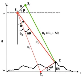
Fig. 1. InSAR geometry.
II. INSAR IMAGINGGEOMETRY
A 2-D SLC SAR image is represented asz=|z| ·ejψ, with its amplitude |z| and phaseψ. The amplitude depends on the transmitter power, the distances of the scatterer to the trans-mitter and the receiver, and the scene reflectivity. On the other hand, the phase depends on the total distance that the signal travels before being received by the receiver antenna. Hence, the phase is mainly composed of two components: 1) the geo-metrical phase due to the total distances between transmitter– scatterer and scatterer–receiver (a deterministic component); and 2) the object’s phase due to the coherent sum of many indi-vidual scatterers, i.e., the scattering phenomenon on the ground (a random component).
In SAR interferometry, the backscattered echo from the same region is received from slightly different positionsS1andS2, as
in Fig. 1, and an interferometric image pair(z1, z2)is obtained.
For the case whereS1transmits and bothS1andS2receive, the
phases of the two SAR images will be ψ1=− 2π λ(2R1)−ψobj1 ψ2=− 2π λ(R1+R2)−ψobj2. (1) Since the random object’s phase components may be as-sumed to be identical for these two images, i.e.,ψobj1≈ψobj2, interferometric phase ψint, which is defined to be the phase
difference between the two images, reflects the difference in the sensor–scatterer distances of the two images, i.e., ΔR=
R2−R1. Unlike the random phase of one SLC image, the
interferometric phase carries particular information about the acquisition geometry as follows:
ψint=ψ1−ψ2= 2π
λΔR≈ −
2π
λ Bsin(θ−β). (2) Due to a nonzero baseline, even a point on the flat Earth yields a nonzero interferometric phase. Then, a point at height δhhas an interferometric phase of
ψint=− 2π
λ Bsin(θ0−β)−
2π
λBcos(θ0−β)δθ (3) where the first term corresponds to the interferometric phase measured in the absence of any topography, and the second term
corresponds to the flattened interferometric phase that reflects the height variations in the scene relative to the flat Earth. Once an interferogram is generated, it is flattened by removing the first term, andψflatis obtained.
Then, together with the knowledge of InSAR parameters, such as baseline B, look angle θ0, and signal wavelength λ,
a change in the flattened interferometric phase corresponds to a change in the terrain height according to the following relation:
δh=−δψflat
λR1sinθ0
2πB⊥ (4)
where theeffective baselineB⊥=Bcos(θ0−β)is the
projec-tion of the interferometric baseline onto the direcprojec-tion perpen-dicular to the line of sight. The height change that leads to a
2π change in the flattened interferometric phase is called the ambiguity height, i.e.,
hamb=
λR1sinθ0
B⊥ (5)
and it can be considered a measure of sensitivity to the topog-raphy. From (5), a longer effective baseline yields a smaller ambiguity height, which means better height sensitivity. How-ever, for long baselines, the spatial decorrelation between the two images should be also considered. As a measure of the similarity between the two images, thecomplex correlationis defined as follows: ρ= E[z1·z ∗ 2] E[|z1|2]E[|z2|2] =|ρc|ejφc (6)
and its magnitude|ρc|is called thecoherence. III. PGINSAR IMAGE
In this letter, the complex-valued flattened InSAR image is used for feature extraction, as previously proposed in [11].
The amplitude of the InSAR image is slightly modified such that the geometric mean of the amplitudes of the two images is used instead of their multiplication as
I=|z1| · |z2| ·ejψflat. (7)
On the other hand, the interferometric phase suffers from being wrapped over principal interval [−π, π). Hence, the observed phase contains 2π phase jumps and has to be un-wrapped to retrieve the original phase. However, since the whole complex-valued images are used in this letter for feature extraction, not their phases, the challenging phase unwrapping operation is avoided. In addition, the idea of an image gradient is adopted for the interferometric phase. Taking the gradient magnitude of the interferometric phase, the number of phase discontinuities is reduced.
Considering the modifications in the InSAR amplitude and phase, a new complex-valuedPGInSARis defined as
PG≡|z1| · |z2| ·ej|∇ψflat| (8)
where |∇ψflat| is the magnitude of the interferometric phase
gradient in the range and azimuth directions. As it is, the PGInSAR image phase can be considered to express how fast the terrain height changes throughout a scene, whereas the InSAR image phase is related to the absolute terrain height [11].
As in [14], ∇ψflat is computed from the real (Ireal) and
imaginary(Iimag)parts of the flattened interferogram as
∇ψflat =
Ireal∇Iimag−Iimag∇Ireal
I2
real+Iimag2
(9) by means of the relationψflat = tan−1
Iimag
Ireal
and the chain rule in the differentiation. Unlike the computation of the gradi-ent directly from the wrapped phaseψflat, the real and
imagi-nary parts, which are usually continuous, yield a phase gradient with less jumps [11].
IV. FEATUREEXTRACTIONBASED ONFRFT In this letter, a nonparametric feature extraction method previously proposed in [13] for the classification of SLC images is adopted to InSAR and PGInSAR images [11]. In that method, the feature descriptor is based on the simple statistics extracted from the FrFT of the SLC image. The FrFT of a functionf(ξ)
is defined as FrFTα(ξ) =Aα·exp(jπξ2cotα) · expjπ(−2xξcscα+x2cotα)f(x)dx Aα= exp [−j(πsgn(sinα)/4−α/2)] |sinα|12 (10) whereα=pπ/2is the transform angle, and0<|p|<2is the transform order of the FrFT. If α= 0 or a multiple of 2π, the FrFT corresponds to the identity operator, and forα=π/2, the FrFT takes the standard Fourier transform [15]. For 2-D images, the transform can be first applied to columns and then to rows, or vice versa, due to the linearity of the FrFT.
Due to the chirplike nature of SLC and InSAR images, a chirplet-based FrFT is expected to be well suited for transform-domain representation. Controlled by the FrFT order, the scaling performed in the phase captures the backscattering and topographic behaviors in SLC and InSAR, respectively [13], [16]. For a given image patch, 17 different FrFT operations are performed with 17 equally spaced transform angles between 0 and π (i.e., Δp= 0.125), and for each of the transformed images, three log cumulants (log mean,log variance, andlog skewness) are computed from its amplitude, yielding a feature descriptor of length 51 [13]. However, for the InSAR and PGInSAR cases, the exploitation of the whole complex data is important in order not to ignore any contribution of the interferometric phase information. Hence, the log cumulants are computed for both the real and imaginary parts of the trans-formed image and then appended to obtain a feature descriptor of length 102 [11].
V. EXPERIMENTALBISTATICSAR IMAGEDATABASE
For patch-oriented classification, an image database of eight different classes is generated. The classes in the database are:C1—agricultural fields; C2—forest;C3—industrial area;
C4—mixed vegetation (forest and agricultural);C5—riverside;
C6—urban-1 (medium-density residential area);C7—urban-2 (high-density buildings); andC8—water body (lakes and ponds). Each class consists of 50 scenes of size200×200pixels. For each scene, there exist three TerraSAR-X add-on for Digital El-evation Measurement (TanDEM-X) image pairs acquired in the
TABLE I
INSAR ACQUISITIONPARAMETERS OF THEDATABASE
bistaticoperation mode with three different effective baselines. That is, the whole database consists of 3 sets of 400 patches, with each set corresponding to a different effective baseline. The orbit direction, the look direction, the look angle, and the wave-length are identical for these acquisitions. These parameters and the corresponding ambiguity heights are tabulated in Table I.
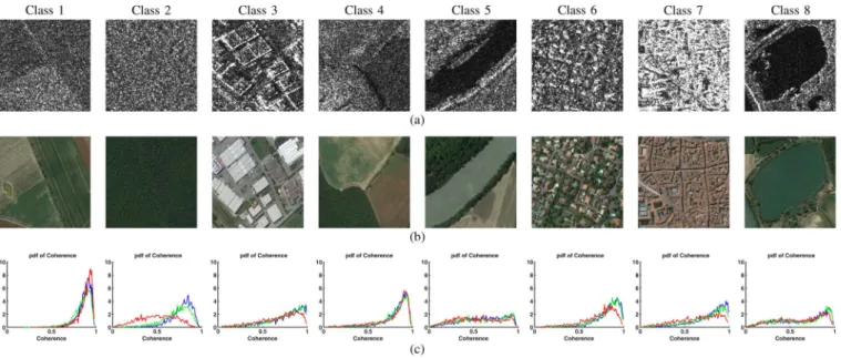
The image patches are from the test site in Toulouse, France. The spatial resolution is about 2 m, i.e., each scene corresponds to an area of 400 m×400 m on the ground. Google Earth has been used as theground truthduring the generation of the database. In Fig. 2, each class in the database is visualized by a sample patch with its quick-look view of the SLC image, together with the corresponding optical Google Earth image.
Due to the bistatic imaging (S1transmits;S1andS2receive
within the same pass), the temporal baseline is quite short (on the order of seconds), resulting in a low temporal decorrelation. Fig. 2(c) illustrates the spatial decorrelation due to the nonzero baseline with the probability density function (pdf) of the in-terferometric coherence values estimated for each sample patch and baseline. It can be seen that a longer baseline yields lower coherence as expected, except for C1 likely due to the seasonal agricultural activities. In addition, for Set 3, the sharp decrease in the C2 coherence may be not only due to the long baseline but also due to the presence of leaves in summer. For a given baseline, C3, C6, and C7 have similar coherence values due to the similar scattering mechanisms, and C5 and C8 have the lowest coherence values due to the specular reflection on water.
VI. CLASSIFICATIONRESULTS
In this letter, a supervised K-nearest neighbor classifier, with a Euclidean distance and k= 1, is used. Four percent of each class, i.e., 2 out of 50 patches, is randomly selected as the training samples for the classifier. Each classification experiment is repeated 100 times with different training sets, and the average of the classification accuracy is reported. A. Performance of SLC SAR, InSAR, and PGInSAR for Set 2
First, the classification performance of the SLC images, that of the InSAR images, and that of the PGInSAR images are compared for Set 2 (a medium baseline), and the results are given in Fig. 3. It can be seen that InSAR is better than SLC with a 15% enhancement in the mean accuracy. PGInSAR introduces further improvement of 10% over InSAR or a total improvement of 27% over SLC.
The F-measures show that InSAR considerably improves all class accuracy values compared with SLC, except for C5 and C8, which is likely due to the specular reflection in these classes. PGInSAR performs the best among all, and the biggest
Fig. 2. Classes in the bistatic SAR image database: C1—agricultural fields; C2—forest; C3—industrial area; C4—mixed vegetation; C5—riverside; C6—urban-1 (medium density); C7—urban-2 (high density); C8—water body. (a) Quick-look views obtained from the amplitude of the master SLC data. (b) Optical Google Earth images as the ground truth. (c) PDFs of the interferometric coherence values computed with a4×4averaging window for three different baselines. Blue curve: Set 1 (a small baseline). Green curve: Set 2 (a medium baseline). Red curve: Set 3 (a long baseline).
Fig. 3. F-measures and mean accuracy of SLC, InSAR, and PGInSAR (Set 2).
TABLE II
CONFUSIONMATRIX FORPGINSAR (SET2)INPERCENTAGE
improvement is achieved for scenes with natural structures such as C1, C2, and C4. The improvements for C3, C6, and C7 are faint due to the strong phase discontinuities present, even in PGInSAR.
Fig. 4. Comparison of the Gabor- and FrFT-based feature descriptors (Set 2).
For a detailed assessment of individual class accuracy values, the confusion matrix for PGInSAR is tabulated in Table II. It can be seen that the misclassifications are mostly observed within the following groups: 1) C1–C2–C4; 2) C3–C6–C7; and 3) C5–C8, which seems to be quite reasonable.
In addition, the FrFT-based feature descriptor is compared with a Gabor-based descriptor (with three scales and four orien-tations), which is a well-known multiscale approach capturing the textural information. The F-measures are given, together with Kappa coefficientsκand standard deviationsσκ, in Fig. 4. The FrFT-based PGInSAR feature descriptor yields the best performance with the highestκand the smallestσκ. Moreover, it seems to be more uniform over all classes than other feature descriptors.
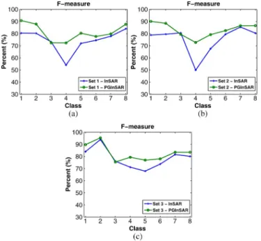
B. Performance of InSAR and PGInSAR for Sets 1, 2, and 3 As the second experiment, the impact of the effective base-line is studied for the InSAR and PGInSAR images. As shown in Fig. 5(a)–(c), for each effective baseline, PGInSAR is better than InSAR. However, with the long baseline, for which the
Fig. 5. F-measures for InSAR and PGInSAR for (a) Set 1 (a small baseline), (b) Set 2 (a medium baseline), and (c) Set 3 (a long baseline).
Fig. 6. F-measures for (a) InSAR and (b) PGInSAR for the three different baselines.
number of fringes and phase discontinuities increase, PGInSAR can no longer perform better than InSAR for C2, and similarly, the improvement is less for C1 and C4.
Furthermore, Fig. 6(a) and (b) shows how InSAR and PGInSAR react to different effective baselines in terms of classification accuracy, respectively. In this figure, it can be seen that, for C2 and C4, the long baseline yields better accuracy despite the low coherence in C2. For C3, C6, and C7, the medium baseline is found to be the best among all. For C5 and C8, the small baseline results in better accuracy. That is, the behavior of a class differs under different effective baselines, as expected. Additionally, the effect of the seasonal changes between acquisitions should be considered. Nevertheless, it is important to note that the PGInSAR feature descriptor is less affected by the effective baseline than the InSAR feature descriptor since the phase discontinuities are reduced compared with InSAR.
VII. CONCLUSION
In this letter, complex-valued InSAR and newly defined PGInSAR images have been used for image classification, where the InSAR phase is related to the absolute height of the
scene and where the PGInSAR phase rather reflects how fast the height changes throughout the image. As the feature descriptor, log cumulants are extracted from the real and imaginary parts of the FrFT coefficients of the complex-valued InSAR and PGInSAR. Classification results show that InSAR and PGInSAR improve the mean accuracy by 15% and 27% com-pared with SLC, respectively.
In addition, the impact of the effective baseline on the clas-sification performance of the InSAR and PGInSAR images is investigated through three interferometric pairs acquired from the same site with different effective baselines. For each base-line, PGInSAR achieves better classification performance than InSAR since the phase discontinuities are reduced. Moreover, it has been observed that, for scenes containing natural structures with smooth phase changes, PGInSAR considerably improves the classification accuracy compared with InSAR. However, the gain of PGInSAR may remain faint for scenes containing man-made objects with abrupt phase changes and even for natural scenes with long baseline acquisitions. The behavior of a class may differ under different baselines, but yet PGInSAR is more robust to the changes in the effective baseline than InSAR.
REFERENCES
[1] U. Wegmuller and C. Werner, “Retrieval of vegetation parameters with SAR interferometry,”IEEE Trans. Geosci. Remote Sens., vol. 35, no. 1, pp. 18–24, Jan. 1997.
[2] A. Elmzoughi, R. Abdelfattah, and Z. Belhadj, “SAR image classification using the InSAR coherence for soil degradation cartography in the South of Tunisia,” inProc. IEEE ICIP, Nov. 2009, pp. 1677–1680.
[3] V. Nizalapur, R. Madugundu, and C. S. Jha, “Coherence-based land cover classification in forested areas of Chattisgarh, Central India, using environmental satellite-advanced synthetic aperture radar data,”J. Appl. Remote Sens., vol. 5, no. 1, Mar. 2011, Art. ID. 059501.
[4] V. Vijaya and G. J. Niveditha, “Classification of COSMO SkyMed SAR data based on coherence and backscattering coefficient,”Int. J. Comput. Sci. Inf., vol. 1, no. 4, pp. 60–63, 2012.
[5] M. E. Engdahl and J. M. Hyyppa, “Land-cover classification using mul-titemporal ERS-1/2 InSAR data,”IEEE Trans. Geosci. Remote Sens., vol. 41, no. 7, pp. 1620–1628, Jul. 2003.
[6] A. B. Suksmono, A. Handayani, and A. Hirose, “Snake in phase domain: A method for boundary detection of objects in phase images,” inProc. IJCNN, 2006, pp. 481–485.
[7] F. Baselice and G. Ferraioli, “Statistical edge detection in urban areas exploiting SAR complex data,”IEEE Geosci. Remote Sens. Lett., vol. 9, no. 2, pp. 185–189, Mar. 2012.
[8] F. Baselice, G. Ferraioli, and D. Reale, “Edge detection using real and imaginary decomposition of SAR data,” IEEE Trans. Geosci. Remote Sens., vol. 52, no. 7, pp. 3833–3842, Jul. 2014.
[9] H. Wang, K. Ouchi, and Y. Q. Jin, “Classification of typhoon-destroyed forests based on tree height change detection using InSAR technology,” inProc. IEEE IGARSS, Jul. 2011, pp. 1247–1250.
[10] A. I. Sharov, K. Gutjahr, and P. E. Pellikka, “Phase gradient approach to the evaluation and mapping of glacier rheology from multi-pass SAR interferograms,” inProc. MultiTemp, Jul. 2004, pp. 154–165.
[11] N. D. Cagatay and M. Datcu,“Scene recognition based on phase gradient InSAR images,” inProc. IEEE ICIP, Paris, France, 2014.
[12] P. A. Rosenet al., “Synthetic aperture radar interferometry,”Proc. IEEE, vol. 88, no. 3, pp. 333–382, Mar. 2000.
[13] J. Singh and M. Datcu, “SAR image categorization with log cumulants of the fractional Fourier transform coefficients,” IEEE Trans. Geosci. Remote Sens., vol. 51, no. 12, pp. 5273–5282, Dec. 2013.
[14] D. T. Sandwell and E. J. Price, “Phase gradient approach to stacking interferograms,”J. Geophys. Res., vol. 103, no. B12, pp. 30 183–30 204, Dec. 1998.
[15] H. M. Ozaktas, O. Arikan, M. A. Kutay, and G. Bozdagi, “Digital compu-tation of the fractional Fourier transform,”IEEE Trans. Signal Process., vol. 44, no. 9, pp. 2141–2150, Sep. 1996.
[16] M. Datcu and J. Singh,“ Phase-scale analysis of complex valued SAR images,” inProc. EUSAR, Jun. 2014, pp. 1121–1124.