Imperial College London Department of Computing
Analysing Directed Network Data
Anida Sarajli´
c
December 2015
Supervisor: Dr. Nataˇsa Prˇ
zulj
Submitted in part fulfilment of the requirements for the degree of Doctor of Philosophy in Computing of Imperial College London
Declaration of Originality
I herewith certify that that the original work submitted in this dissertation is my own and that all material in this dissertation which is not my own work has been properly acknowledged.
Anida Sarajli´c
Copyright Declaration
The copyright of this thesis rests with the author and is made available under a Creative Commons Attribution Non-Commercial No Derivatives licence. Researchers are free to copy, distribute or transmit the thesis on the condition that they attribute it, that they do not use it for commercial purposes and that they do not alter, transform or build upon it. For any reuse or redistribution, researchers must make clear to others the licence terms of this work.
Abstract
The topology of undirected biological networks, such as proteprotein in-teraction networks, or genetic inin-teraction networks, has been extensively explored in search of new biological knowledge. Graphlets, small connected non-isomorphic induced sub-graphs of an undirected network, have been particularly useful in computational network biology. Having in mind that a significant portion of biological networks, such as metabolic networks or transcriptional regulatory networks, are directed by nature, we define all up to four node directed graphlets and orbits and implement the directed graphlet and graphlet orbits counting algorithm. We generalise all exist-ing graphlet based measures to the directed case, definexist-ing: relative directed graphlet frequency distance, directed graphlet degree distribution similarity, directed graphlet degree vector similarity, and directed graphlet correlation distance. We apply new topological measures to metabolic networks and show that the topology of directed biological networks is correlated with biological function. Finally, we look for topology–function relationships in metabolic networks that are conserved across different species.
I dedicate this dissertation to my parents and my brother for all
their love and support.
Acknowledgements
I wish to thank my supervisor, Dr. Nataˇsa Prˇzulj, for giving me the opportunity to join her research group at Imperial College London and to work in this exciting research environment. I am grateful for Dr. Prˇzulj’s guidance and support on my research, as well as for her passion for science, motivating me to always strive for more. With this guidance, I developed research skills which I hope to always be proud of. I also wish to thank Dr. N¨oel Malod-Dognin, Dr. Prˇzulj’s post-doctoral researcher, for all insightful discussions and guidance during my work on this dissertation. Also, I would like to thank members of my viva examination committee, Prof. Dr. Jan Baumbach and Prof. Dr. Murray Shanahan, for all the useful comments which led to the improved final version of this manuscript.
I am especially grateful to all former and current fellow PhD students: Dr. Vuk Janji´c, Vladimir Gligorijevi´c, Dr. ¨Omer Nebil Yaverˇoglu and Dr. Kai Sun, for genuine friendship, fruitful discussions and all their support.
I sincerely thank Prof. Djordje Radak, Prof. Charles Coombes and Dr. Aleksandra Filipovi´c for the collaborative work on several journal publications during my research as a member of Dr. Prˇzulj’s group.
I acknowledge European Research Council (ERC) Starting Independent Researcher Grant 278212 (2012-2017) for the funding of my studies.
Finally, I am very grateful for my dearest, my family, their understanding, love and support.
Contents
Contents 6 List of Tables 9 List of Figures 12 1 Introduction 15 1.1 Motivation . . . 15 1.2 Dissertation Outline . . . 171.3 Networks and Network Properties . . . 18
1.3.1 Global Network Properties . . . 21
1.3.2 Local Network Properties . . . 25
1.3.3 Graphlet-based Measures for Analysing Network Topology . . . . 27
1.4 Random Network Models . . . 31
1.5 Biological Networks . . . 36
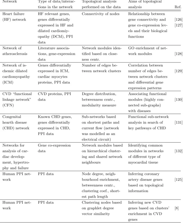
2 Undirected Biological Networks in Researching Complex Diseases: Cardiovascular Disease (CVD) Case Studies 41 2.1 Review of Network-based Approaches in Researching Cardiovascular Dis-eases . . . 42
2.1.1 Exploring Disease Through Network Topology . . . 42
2.2 CVD Case Studies . . . 47
2.2.1 Network Topology Reveals Key Cardiovascular Disease Genes . . 47
2.2.2 Network Wiring of Pleiotropic Kinases Yields Insight into the Re-lationship between Diabetes and Aneurysm . . . 60
2.3 Conclusions . . . 75
3 Directed Graphlet-based Methods 78
3.1 Methods . . . 78
3.1.1 Directed Graphlets and Graphlet Orbits . . . 78
3.1.2 Directed Graphlet-based Measures . . . 81
3.1.3 Redundancies between Directed Graphlet Orbits . . . 86
3.1.4 Implementation of Directed Graphlets and Orbits Counting Al-gorithm . . . 89
3.2 Evaluation of Directed Graphlet-based Methods for Network Comparison using Synthetic Data . . . 93
3.2.1 Standard Methods for Evaluation of Clustering Performance . . 93
3.2.2 Clustering Directed Model Networks . . . 94
3.2.3 Noise Tolerance . . . 101
3.3 Conclusions . . . 106
3.4 Author’s Contributions . . . 106
4 Application of Directed Graphlet-based Methods to Metabolic Net-works 108 4.1 Topology-based Clustering of Metabolic Networks of Eukaryotes Agrees with Taxonomic Classification . . . 108
4.1.1 Methods . . . 109
4.1.2 Results . . . 111
4.1.3 Comparison with Undirected Metabolic Networks . . . 117
4.2 Similar Wirings around Enzymes in Metabolic Network of H. Sapiens Correspond to Similar Biological Functions . . . 123
4.2.1 Methods . . . 123
4.2.2 Results . . . 124
4.3 Topology–Function Relationships in Metabolic Networks are Conserved across Different Species . . . 126
4.3.1 Methods . . . 127
4.3.2 Results . . . 132
4.4 Conclusions . . . 149
4.5 Author’s Contributions . . . 150
5 Conclusions and Future Directions 152 5.1 Conclusions . . . 152
Bibliography 159
Appendices 183
A Appendix to Chapter 2 184
A.1 Literature Validations of Predicted CVD Genes . . . 184
B Appendix to Chapter 3 186
B.1 The Source Code for the Directed Graphlets and Orbits Counter . . . . 186
C Appendix to Chapter 4 211
C.1 GO Enrichment of Enzyme Clusters in the Metabolic Network ofH. sapiens211 C.2 GO Enrichment of Enzyme Sets Corresponding to Characteristic
List of Tables
1.1 Databases of molecular interaction data. . . 37
2.1 Methods that explore the topology of biological networks in CVD research. 46 2.2 Functional annotation of the ten key cardiovascular disease genes. . . . 52 2.3 Predicted CVD genes. . . 53 2.4 The Key Cardiovascular Disease Genes that are known drug targets. . . 56 2.5 Pathways related to aneurysm. . . 65 2.6 Pathways related to atherosclerosis. . . 66 2.7 The 24 pathways containing genes that participate in specific genetic
interactions. . . 67 2.8 The 16 broker genes participating in specific genetic interactions. . . 73
3.1 Complete list of orbit dependencies for all directed 2 to 4 node graphlets. 83 3.2 AU C, AU P R and AU CEP Q=10 scores for clustering model networks
when comparing all-to-all networks. . . 97 3.3 AU C, AU P R and AU CEP Q=10 scores for clustering model networks
when comparing the networks of same size and density. . . 100
4.1 AUC scores for clustering metabolic networks according to Kingdom, Phylum, Class, Order, Family and Genus levels of taxonomic classification.113 4.2 AUPR scores for clustering metabolic networks according to Kingdom,
Phylum, Class, Order, Family and Genus levels of taxonomic classification.115 4.3 Comparison of AUC scores for clustering undirected and directed metabolic
networks according to Kingdom, Phylum, Class, Order, Family and Genus levels of taxonomic classification. . . 120 4.4 Comparison of AUPR scores for clustering undirected and directed metabolic
networks according to Kingdom, Phylum, Class, Order, Family and Genus levels of taxonomic classification. . . 122 4.5 Number of enriched GO terms in clusters in H. sapiens metabolic
4.6 Number of enriched GO terms in clusters in H. sapiens metabolic net-work; 19 clusters. . . 125 4.7 Metabolic networks of H. sapiens and four model organisms. . . 127 4.8 Number of Common GO terms per analysed species pair. . . 130 4.9 Number of GO terms with statistically significant topology–function
re-lationships (statistically significant structure association strengths). . . . 131 4.10 Number of genes with predicted BP annotations. . . 133 4.11 The number of topologically orthologous GO terms per pairwise
experi-ment. . . 136 4.12 Topologically orthologous biological processes across species pairs. . . . 137
C.1 GO term enrichment of 4 enzyme clusters inH. sapiens metabolic network.213 C.2 GO term enrichment of 19 enzyme clusters inH. sapiens metabolic network.221 C.3 Case study: Purine nucleotide metabolic process. GO term enrichment
of enzymes touching orbit 5 in H. sapiens metabolic network. . . 223 C.4 Case study: Purine nucleotide metabolic process. GO term enrichment
of enzymes touching orbits 10 or 12 in H. sapiens metabolic network. . 224 C.5 Case study: Purine nucleotide metabolic process. GO term enrichment
of enzymes touching orbit 5 in M. musculus metabolic network. . . 225 C.6 Case study: Purine nucleotide metabolic process. GO term enrichment
of enzymes touching orbits 10 or 12 in M. musculus metabolic network. 226 C.7 Case study: Purine nucleotide metabolic process. GO term enrichment
of enzymes touching orbit 5 in D. melanogaster metabolic network. . . . 226 C.8 Case study: Purine nucleotide metabolic process. GO term enrichment
of enzymes touching orbits 10 or 12 in D. melanogaster metabolic network.227 C.9 Case study: Ribose phosphate metabolic process. GO term enrichment
of enzymes touching orbit 5 in H. sapiens metabolic network. . . 228 C.10 Case study: Ribose phosphate metabolic process. GO term enrichment
of enzymes touching orbits 10 or 12 in H. sapiens metabolic network. . 229 C.11 Case study: Ribose phosphate metabolic process. GO term enrichment
of enzymes touching orbit 5 in M. musculus metabolic network. . . 230 C.12 Case study: Ribose phosphate metabolic process. GO term enrichment
of enzymes touching orbits 10 or 12 in M. musculus metabolic network. 231 C.13 Case study: Ribose phosphate metabolic process. GO term enrichment
C.14 Case study: Ribose phosphate metabolic process. GO term enrichment of enzymes touching orbits 10 or 12 in D. melanogaster metabolic network.232 C.15 Case study: Cyclic nucleotide metabolic process. GO term enrichment
of enzymes touching orbit 5 in H. sapiens metabolic network. . . 232 C.16 Case study: Cyclic nucleotide metabolic process. GO term enrichment
of enzymes touching orbits 10 or 12 in H. sapiens metabolic network. . 233 C.17 Case study: Cyclic nucleotide metabolic process. GO term enrichment
of enzymes touching orbit 5 in M. musculus metabolic network. . . 234 C.18 Case study: Cyclic nucleotide metabolic process. GO term enrichment
of enzymes touching orbits 10 or 12 in M. musculus metabolic network. 235 C.19 Case study: Cyclic nucleotide metabolic process. GO term enrichment
of enzymes touching orbit 5 in D. melanogaster metabolic network. . . . 236 C.20 Case study: Cyclic nucleotide metabolic process. GO term enrichment
List of Figures
1.1 Different topologies with the same degree distributions. . . 21
1.2 73 Graphlets and graphlet degree vector (GDV) of a node. . . 28
2.1 Using network topology to uncover elements involved in a disease . . . . 44
2.2 Method for inferring the key CVD genes - Flowchart . . . 48
2.3 The distribution of GDV similarity of protein pairs in the human PPI network. . . 55
2.4 Summary of the results of the CVD study. . . 56
2.5 Work-flow of the aneurysm-diabetes study. . . 62
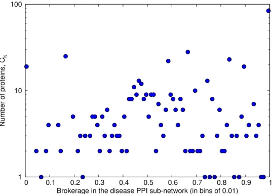
2.6 Distribution of brokerage values in the disease PPI sub-network. . . 70
2.7 Statistically significant brokerage values in the disease sub-network. . . 71
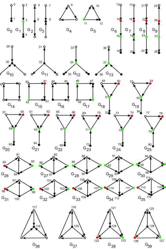
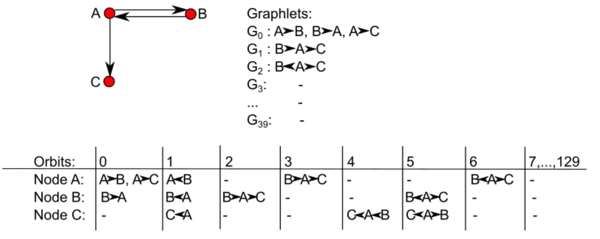
3.1 40 Directed Graphlets and 129 orbits. . . 79
3.2 Inducing directed graphlets from the network with anti-parallel pairs of arcs. . . 81
3.3 Illustration of the redundancies between directed graphlet orbits 0, 6 and 11. . . 87
3.4 Model clustering performance when comparing all-to-all networks. . . . 98
3.5 Model clustering performance when comparing networks of the same size and density. . . 99
3.6 Model clustering performance when the similarity scores are obtained at random. . . 100
3.7 Effects of missing network edges on model clustering performance of dif-ferent network distance measures. . . 103
3.8 Effects of rewiring networks on model clustering performance of different network distance measures. . . 104
3.9 Effects of adding network edges on model clustering performance of dif-ferent network distance measures. . . 105
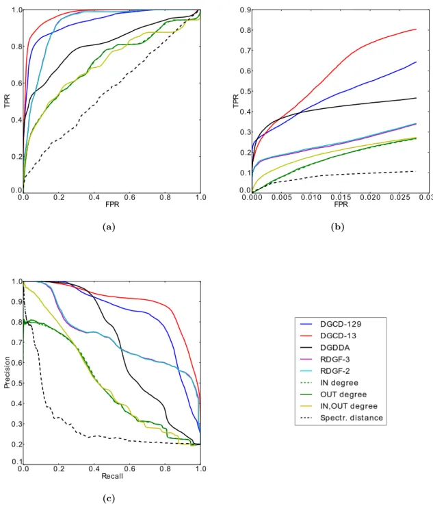
4.1 ROC curves for clustering of directed metabolic networks according to (a) kingdom, (b)phylum. . . 111 4.1 ROC curves for clustering of directed metabolic networks according to
(c) class, (d) order, (e) family and (f) genus. . . 112 4.2 Precision-recall curves for clustering of directed metabolic networks
ac-cording to (a) kingdom, (b)phylum. . . 113 4.2 Precision-recall curves for clustering of directed metabolic networks
ac-cording to (c) class, (d) order, (e) family and (f) genus. . . 114 4.3 Precision-recall curves for clustering of directed metabolic networks using
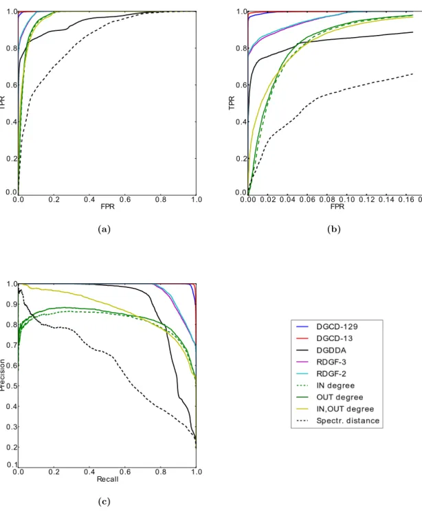
random similarity scores. . . 115 4.4 Phylogenetic tree of eukaryotes, obtained using DGCD-13 measure. . . . 117 4.5 Comparison of ROC curves for clustering of undirected and directed
metabolic networks according to (a) kingdom, (b)phylum. . . 118 4.5 Comparison of ROC curves for clustering of undirected and directed
metabolic networks according to (c) class, (d) order, (e) family and (f) genus. . . 119 4.6 Comparison of precision-recall curves for clustering of undirected and
directed metabolic networks according to (a) kingdom, (b)phylum. . . . 120 4.6 Comparison of precision-recall curves for clustering of undirected and
directed metabolic networks according to (c) class, (d) order, (e) family and (f) genus. . . 121 4.7 ROC curves for predicting GO annotations. . . 134 4.8 Number of GO terms per structire association strength value. . . 135 4.9 Orbit contribution strength profiles of the topologically orthologous
bio-logical processes between H. sapiens and D. melanogaster. . . 139 4.10 Illustration of topological patterns linked to some of the topologically
orthologous GO terms. . . 140 4.11 Parent-child relationships between topologically orthologous biological
processes in in Gene Ontology tree. . . 141 4.12 GO enrichment around enzymes touching orbit 6, that are annotated
with purine nucleotide metabolic process. . . 143 4.13 GO enrichment around enzymes touching orbit 11, that are annotated
with purine nucleotide metabolic process. . . 144 4.14 GO enrichment around enzymes touching orbit 6, that are annotated
4.15 GO enrichment around enzymes touching orbit 11, that are annotated with cyclic nucleotide metabolic process. . . 149
1 Introduction
1.1 Motivation
A network (also called a graph) is a common model of a set of objects and their inter-actions for describing and analysing data in numerous research areas. Different graph theoretic approaches are used for analysing network data.
Computational network biology is an emerging research area that complements tra-ditional biology and medicine. Computational analysis on ever-growing amounts of available biological data offers new insight into research on the development of living organisms, research on human diseases and the discovery of new drug targets. A number of large-scale data sets were generated as a result of recent advances in high-throughput techniques. These molecular data include information on interactions between biological macromolecules, such as protein–protein interactions (PPI), genetic interactions (GI), enzyme-substrate relationships and pathway maps. The concept of networks has been introduced in systems biology as it accurately captures the inner workings of many com-plex biological systems and reduces the comcom-plexity of biological data that is required for performing computational analyses. Also, the fact that a specific network topology comes as a direct consequence of biological processes occurring between the elements of the underlying system, highlights the importance of the topology as a valuable source of new biological knowledge. Graph theoretic approaches help to identify topological properties which differ from the wiring which can be expected at random, revealing the connection between a specific topological characteristic and a related biological function or phenotype, such as disease.
The majority of current publicly available biological networks are undirected net-works. For example, PPI networks, where nodes correspond to proteins and edges are placed between two proteins if they physically interact, are networks with a highly ex-plored topology. It was shown that proteins which are close in the PPI network are more likely to perform the same function [1] which was used for inferring functions of unannotated proteins: the direct neighbourhoods of proteins [1], n–neighbourhoods of proteins [2], and shared neighbours of proteins [3] were examined looking for the most
common functions among annotated direct neighbours. Several other methods have shown that PPI network topology around proteins is a predictor of their function or their involvement in a disease [4–6].
Graphlets, small connected non-isomorphic induced sub-graphs of an undirected net-work, first introduced by Prˇzuljet al.[7], have been particularly useful: the local topol-ogy around a protein in a PPI network was summarised into a topological “signature” of a protein –graphlet degree vector (GDV)[4] and the similarity of these protein “sig-natures” is a good indicator that proteins belong to the same protein complex, perform similar biological functions, are coexpressed, involved in the same diseases, and are part of the same sub–cellular components [4]. This topological measure of similarity was used for predicting new melanogenesis related genes that were phenotypically validated [5] and for identifying key cardiovascular disease genes [8]. In addition, Gligorijevi´c et al.[9] developed an integrative model for gene ontology (GO) reconstruction and gene function prediction. They show that the GDV similarity between nodes contains com-plementary information to the connectivity patterns, and integrating these two sources of information boosts the quality of the integrative model by increasing the performance of gene function and GO term association predictions.
In recent years, there is a growing trend in completing and exploring biological net-works that are directed by nature, such as transcriptional regulatory netnet-works, metabolic networks, and effective connectivity brain networks [10–12]. Various network proper-ties and measures exist for topological analysis of directed networks, such as properproper-ties based on nodes’ degrees or network spectra. However, directed graphlets are still not defined. In this dissertation, we define directed graphlets and directed graphlet-based heuristics for analysis of directed networks. Furthermore, we show that our measures outperform common existing measures for directed networks comparison. Finally, we apply these new topological measures to show that topology of directed metabolic net-works is correlated to biological information.
As was the case with the undirected graphlets [13], application of directed graphlets and derived measures is certainly not limited to computational biology. For instance, sociology, economy and technology are just some of the many research areas in which the underlying complex interactions can be modelled using directed networks: social interaction networks, world trade networks, citation networks, autonomous system net-works etc. The set of new measures that we propose in this dissertation opens up a window of opportunities for exploring these research areas from a new perspective.
1.2 Dissertation Outline
In the remainder of this section, we introduce undirected and directed networks and and give an overview of graph-theoretic measures for local network topology analysis, network comparison and network modelling. In addition we provide a brief description of different types of biological networks, as all applications presented in Chapter 4 of this dissertation involve biological networks.
We use Chapter 2, to show that it is possible to tackle open problems in biology and medicine using graph theoretic approaches on undirected biological networks. We first give a short review of network-based approaches in research on complex diseases, in particular cardiovascular diseases (CVD), as they are a leading health problem world-wide [14]. We then present two case studies where we analyse CVDs using undirected biological networks: (1) In the first study, we apply graphlet-based measures to the human PPI network to identify key genes involved in CVDs.(2) In the second study, we use human PPI and genetic networks to explore the reasons behind the protective role of diabetes against the development of aneurysm. Using a topological measure of brokerage - a measure that identifies “weak” points in a network, we find kinases that, conditioned with diabetes pathways, can influence disruption of pathways responsible for the development of aneurysm.
Motivated by the growing amounts of available directed biological network data, and the usefulness of topological analysis in biological research described in Chapters 1 and 2, in Chapter 3 we introduce our new methodology for the analysis of directed networks. We define directed graphlets and generalise the following undirected graphlet-based measures to the directed case: relative graphlet frequency distance, graphlet degree distribution similarity, graphlet degree vector similarity, and graphlet correlation distance. Using synthetic networks and model network clustering, we then show that directed graphlet-based measures outperform commonly used measures for comparison of directed networks. In addition, in case of directed networks without anti-parallel pairs of arcs, we find orbits that are redundant among up-to-four node graphlets.
In Chapter 4, we demonstrate the use of the new network measures introduced in Chapter 3 by applying them to directed metabolic networks. Namely, we evaluate the quality of topology-based clustering of metabolic networks of eukaryotic species accord-ing to their taxonomic classification and confirm that graphlet-based measures outper-form other common measures for directed network comparison. Further on, we show that similar local topologies around genes in the human metabolic network correspond to similar biological functions. Motivated by this finding we use directed graphlets to
further explore metabolic networks of several eukaryotic species and find conserved rela-tionships between topology around genes and their biological functions across different species. We also show the predictive power of a gene’s directed graphlet signature in a metabolic network for annotating the gene with biological functions.
Finally, in Chapter 5, we conclude the dissertation with a summary of our contribu-tions, and discuss future work.
1.3 Networks and Network Properties
A network, also called a graph, is a mathematical object denoted as a pair G={V, E}, whereV is a set of vertices (nodes) and E is a set of edges that connect pairs of nodes according to some relationship between them [15]. In an undirected graph, edges are unordered pairs of vertices. In adirected graph, edges are ordered pairs of vertices, often called arcs, directed edges, or arrows. A directed edge or arc e= (x, y) is considered to be directed from xtoy, wherey is called the head andx is called the tail of the arc,y
is a direct successor of x, and xis a direct predecessor of y.
A graph can be represented as the |V| × |V|dimensional adjacency matrix A. In an undirected graph, the entryAij from matrixA takes a non-zero value or a zero value if
the nodes iand j are connected with an edge or not, respectively [15, 16]. In a directed graph,Aij is the number of arcs from nodeito nodej. In a weighted graph the values
in the matrix can be used to represent the edge weights. A graph can also be presented in the format of an adjacency list: it is a |V| ×2 dimensional array representing nodes in the network, with each node linked to a list of nodes that it is connected to. In case of a weighted network an additional list of edge weights is necessary for each node.
The choice of network representation depends on computing requirements and the type of the network. For example, for more sparse networks the adjacency list is more memory efficient then the adjacency matrix. Also operations of adding or deleting nodes from a network have a high computational cost in case of adjacency matrix because the size of the matrix changes and it needs to be allocated again. However, operations on edges are more computationally efficient if performed on adjacency matrices because they require only a change in the value of the existing matrix elements. Another advan-tage of matrix representation is that additional network information can be encoded in the matrix. For example, the Laplacian matrix of a network contains information on nodes degrees in the diagonal elements. It is calculated as the difference between: (1)the matrix containing only nodes’ degrees as the diagonal elements and (2)the adjacency matrix.
Depending on the type of edges - whether they have an orientation or not - networks (graphs) can be directed, undirected, or mixed. A network is weighted if values are assigned to network edges. Note that in the case of an undirected graph the adjacency matrix is symmetric, whereas in the case of a directed or mixed graph it is not. Here, we list common network concepts:
• Multiple edges, also called parallel edges, are two or more edges with the same pair of endpoints. In directed networks, multiple edges are edges with the same ordered pair of endpoints [17].
• A loop is an edge whose endpoints are equal.
• A simple graph is an unweighed graph containing no loops or multiple edges. A directed graph is simple if each ordered pair of vertices is the head and tail of at most one edge [17].
• A neighbourhood of nodei is a set of nodes adjacent to node i.
• A path is a simple graph whose vertices can be ordered so that two vertices are adjacent if and only if they are consecutive in the list [17]. A directed path is a simple directed graph whose vertices can be linearly ordered so there is an edge with tail u and head v if and only if v immediately follows u in the vertex ordering [17].
• The shortest path between nodes, also called a geodesic path [18], is such that no shorter path between these nodes exists in the network.
• A graph is connected if each pair of vertices in the graph belongs to a path, otherwise, the graph is disconnected [17]. A directed graph is weakly connected if its underlying undirected graph is connected. A directed graph is strongly connected if for each ordered pair (u, v) of vertices, there is a directed path from
u tov [17].
• A cycle is a path that starts and ends in the same node.
• An arc(x,y) inverted in a directed graph is arc(y, x).
• An anti - parallel pair of arcs is a pair of arcs such that one’s head/tail is the other’s tail/head (e.g. arcs (x, y) and (y, x)).
• An induced sub-graph of graph G(V, E) is a sub-graph G0(V0, E0) such that it contains all edges in G between verticesV0.
• A partial sub-graph of graphG(V, E) is a sub-graph G0(V0, E0) such that it does not contain all edges in G between verticesV0.
• An isomorphism of graphs G and H is a bijectionf between the nodes of G and H such that any two vertices i and j from G are adjacent in G if and only if f(i) and f(j) are adjacent in H.
• A sub-graph isomorphism problem is a task where for given networks G and H, it has to be determined whether graph G contains a sub-graph that is isomorphic to H. This problem is NP-complete [19] which means that there are no polynomial time exact solutions. N P denotes a set of all decision problems whose solutions can be verified in polynomial time. P denotes a set of all decision problems whose solutions can be found in polynomial time. A problem p is NP-complete if it is in N P and if every problem in N P is reducible to p in polynomial time [20]. Note that there is still no proof whether NP-complete problems are solvable in polynomial time (P = N P) and this is one of the great unsolved problems of mathematics [21, 22]. In the case that P = N P, the sub-graph isomorphism problem would be solved in polynomial time.
Below are listed the properties which summarise the topological characteristics of net-works. First we address the global network properties, which give an overview of the network with respect to all its nodes and edges. Then we address the local network properties, which describe the network topology using sub-graphs, namely motifs [23] or graphlets [7]. We also list all network distance measures that are based on the discussed properties. The distance measures address the network topology comparison problem and quantify the topological correspondence between the two networks or between the local topologies around nodes in the network.
Note that in this dissertation we do not address the network alignment problem and thus we do not discuss existing network alignment algorithms. Network alignment algorithms are another approach for the network comparison problem with the goal of producing a mapping between nodes of two networks such that the correspondence between the edges of the compared networks is maximised.
1.3.1 Global Network Properties
• Degree distribution. Thedegree kof a node is the number of edges attached to that node. The degree distribution d(k) shows the probability that a randomly selected node has degreek, for allk≥0 [16]. Nodes with the highest degree values are called networkhubs. Note that this is a very simplistic notion of a hub and that identification of hubs in real world networks is often based on multiple network attributes [24]. For example, in a brain network with vertices corresponding to brain regions and edges representing inter-regional pathways, hub brain regions were identified based on node degree, motif fingerprint, betweenness and closeness centrality of nodes in the network [25]. Another example is a directed network of web-pages [26], where nodes are ranked based on the relevancy of information they contain. In that network, a hub was defined as a vertex that points to highly ranked vertices [26, 27].
The degree distribution captures only one aspect of network topology; networks with completely different topologies can have the same degree distributions [28], as illustrated in Figure 1.1. In social networks the degree of a node is sometimes referred to as degree centrality, to emphasise its use as a centrality measure [18]. The centrality measures will be discussed further later on. Theaverage degree of a network is the arithmetic average of the degrees of all nodes in the network.
In directed networks there exist two different types of degrees for a node: (1) the in-degree of a node is defined as the number of edges that are pointing to the node, (2) the out-degree is defined as the number of edges that are pointing from the node. The total degree of the node in the directed network is given as the sum of itsin- andout- degrees.
Figure 1.1. Different topologies with the same degree distributions. The topologies of two graphs shown in the figure differ: Graph A consists of two connected components (two triangles), while Graph B is a single connected component. Still, both graphs have the same number of nodes (six), the same number of edges (six), and the same degree distribution (each of the six nodes in the graph has the degree of two).
When comparing networks using their degree distributions, the most common approach is computing the Euclidian distance between the distributions of the two networks. Ifdi anddj are the degree distributions of the two networksI and
J being compared, then the Euclidian distanceEdist(di, dj) is given as:
Edist(di, dj) = v u u t max(ki,kj) X k=0 (di(k)−dj(k))2;. (1.1)
where ki and kj are maximum degrees in networks I and J, respectively. It is
possible to differently weight or normalise distributions before computing the Eu-clidian distance in order to reduce or emphasise the significance of some elements in the distribution.
• Clustering spectrum, Average clustering coefficient. The clustering coef-ficient is the probability that two nodes j and k, connected to node i, are also connected among themselves [29, 30]. The clustering coefficient of a node i is defined by
Ci =
2Ki
ki(ki−1)
, k≥2; (1.2)
where Ki denotes the number of edges between neighbours of the node i and ki
denotes the degree of the node i. Ci = 0 for k < 2. The average clustering
coefficient of a network is calculated as the average value of clustering coefficients over all nodes in the network [31]:
¯ C= 1 n n X i=1 Ci, (1.3)
where n denotes number of nodes in the network. Clustering spectrum of the network, C(k), is the distribution of the averages of clustering coefficients of all nodes of degree kin the network, over all k.
• Average path length. The shortest path lengthlij between nodesiandjis the
minimum number of edges that form a connected path between these nodes. The average path length in the network is defined as
hli= 2
N(N −1)
X
hi,ji
lij; (1.4)
• Network diameter and network radius. In a connected graph, the eccentric-ity of a node is the maximum distance between the node and any other node in the graph. The maximum eccentricity is denoted as the network diameter. The minimum graph eccentricity is denoted as the network radius. Note that the di-ameter of the network is also defined as the maximum distance within the network (described above): D = max(lij). Here we also mention the small-world
prop-erties of a network [33]. In small world networks, the shortest distance between two randomly chosen nodes grows proportionally to the logarithm of the number of nodes in that network [29]. Social networks and some biological networks ex-hibit small-world network characteristics—they have much smaller diameters than would be expected at random [29].
• Centrality Measures
– Degree centrality. As mentioned above, degree centrality is equivalent to the degree of a node. In terms of centrality, the degree relates to the importance of a node, based on the number of neighbouring nodes.
– Eigenvector centrality. This is an extension of degree centrality: the im-portance of the vertex increases based on the importance of its neighbouring nodes [18]. Relative scores are assigned to nodes based on the concept that having high-scoring nodes as neighbours contributes more to the score of the node than having low-scoring neighbours. Eigenvector centrality of a nodei
can be calculated using [34]:
xi=k1−1
X
j
Aijxj; (1.5)
where A is the adjacency matrix of the network, and k1 is the largest of the
eigenvalues of matrix A. The eigenvector centrality of a node has a higher value if the node has many neighbours, and/or his neighbours areimportant. Another generalisation of degree centrality is Katz centrality [35] of a node, which measures the number of all nodes that can be connected with the node through a path. The contributions of more distant nodes are penalised using an attenuation factorα∈(0,1). The centrality measure with the trade name PageRank [36] is used as a central part of Google’s web ranking technology. It can be observed as a variation of Katz centrality where the centrality that a node derives from its neighbours is proportional to their centrality divided by their out-degree [18] (a network of webpages being a directed network).
Spectral network theory analyses the topology of a network by using the eigen-values and eigenvectors of network matrices. If X is a matrix describing the network (Laplacian or adjacency matrix) [37], then the eigendecomposition of X is given asX =φλφT, whereλ=diag(λ1, λ2, ..., λn) is the diagonal matrix
with the sorted eigenvalues as elements andφ= (φ1|φ2|...|φn) is the matrix
of columns containing sorted eigenvectors. Thegraph spectrum is defined as the set of eigenvalues s = λ1, λ2, ..., λn, where λ1 ≤ λ2 ≤ ... ≤ λn. Note
that the eigenvalues of a matrix are real numbers in the case of a symmetric matrix, i.e. A =AT, which means that the spectra of undirected networks are real numbers. Two networks are called cospectral if they have the same eigenvalues.
Networks can be compared based on their spectra by calculating thespectral distance. If s1 and s2 are network spectra of two graphsG and H, then the spectral distance is defined as the Euclidian distance d(G, H) between the spectras1 and s2 [37]: ds(G, H) = s X i (λ1 i −λ2i)2; (1.6)
If the lengths of the spectra are different, 0 valued eigenvalues are added to the smaller spectrum while preserving the correct magnitude ordering. Graph spectrum can be computed using Laplacian matrix, normalised Laplacian matrix, adjacency matrix, shortest path length matrix etc. It was shown that the spectral distance computed using Laplacian matrices is the most appropriate for classification and clustering experiments [37]. Thus, in our experiments we use spectral distance based on Laplacian matrices and denote it simply as spectral distance.
– Closeness centrality. The farness of a node is defined as the sum of its shortest paths to all other nodes, and its closeness is defined as the inverse of the farness [38]. For nodev it is calculated as:
Cc(v) =
1
P
u∈V dist(u, v)
; (1.7)
where dist(u, v) is the distance between nodes u and v and V is the set of nodes in the network. Therefore, the more central the node is in a network, the lower its total distance to all other nodes is.
– Betweenness centrality. This quantifies the number of times a node lies on the shortest path between two other nodes in the network [39]. Betweenness centrality of a nodeican be calculated using [18]:
xi = X s6=i,t6=i,s6=t nist gst , (1.8)
where nist is the number of shortest distances between s and t that pass through node i, and gst is the total number of shortest distances between
nodess and t. The convention is that nist
gst equals 0 ifgst is 0. Equation 1.8
can be normalised by dividing it with the total number of node pairs in the network.
– K-shell decomposition. K-shell decomposition of a network is conducted by iteratively removing and grouping nodes based on their degrees. The steps of the algorithm are:
1. All nodes of degree ≤ 1, along with their edges, are removed from the network. All removed nodes form the 1-shell of the network;
2. In the resulting network, all nodes of degree≤2, along with their edges are removed from the network, forming the 2-shell;
3. The decomposition process is repeated until all nodes are assigned to one of the k-shells.
The largest value ofk for which the resulting network is not empty is called
kmax, and the corresponding sub-network is called kmax-core, or the core of
the network. Nodes corresponding to higher degree shells are more central in the network, but are not necessarily hubs [40].
1.3.2 Local Network Properties
• Network Motifs. A network motif is a pattern that occurs at a statistically significant frequency in the network [23]. Motifs are partial sub-graphs. The pro-cess of finding motifs is as follows: (1) occurrences of different patterns of interest in a network are counted, (2) the network is randomised conserving the nodes degrees, (3) the frequencies of the patterns are counted in the randomised net-work, where the null model is Erd¨os-Renyi (ER) random network model (random network models will be described in more detail in section1.4), (4) steps 2 and 3 are repeated to find the frequency distribution for topological patterns in the
set of randomised networks, (5) statistical significance of the frequency of each sub-graph in the original network is determined from the frequency distributions obtained in (4) using the Z-score as follows [41]:
Zi =
(Nreali−< Nrandi >)
std(Nrandi)
, (1.9)
whereNreali is the number of times the sub-graph appears in the original network,
and < Nrandi > and std(Nrandi) are the mean and standard deviation of its
appearances in the randomised networks, respectively. The normalisedZ-score of the sub-graph in question is called the sub-graph’ssignificance profile SP and for a sub-graphiit is calculated as:
SPi =
Zi
(P Zi2)12
. (1.10)
This normalisation emphasises the relative significance of sub-graphs, rather than the absolute. Normalisation enables the comparison of networks of different sizes because the motifs in large networks tend to have higher Z values than those in smaller networks. It is possible to group networks according to similar motif-spectra [41]. Obviously, network motifs can be identified both for directed and undirected networks and indicate the main organisational principles within a net-work. An example is the feed forward loops that are shown to be over-represented in signalling networks [42] which is in line with how the signals are propagated though such networks. A drawback of network motifs is that they are dependent on the choice of a network null model [43]
• Graphlets. Graphlets are the small, connected, non-isomorphic induced sub-graphs of a network first introduced by Prˇzulj et al. [7]. Recall that an induced sub-graph of a networkGis a sub-graph that contains all edges between its nodes which are present inG; this is different to a partial sub-graph that contains only some of these edges (above defined network motifs are partial sub-graphs). They can appear in the network at any frequency and thus are not dependent on a null model. All 30 two to five node graphlets, denoted by G0 to G29 are shown
at the top of Figure 1.2. Three highly sensitive measures of network local struc-tural similarities are based on graphlets: the Relative Graphlet Frequency Dis-tance (RGF distance) [7], Graphlet Degree Distribution Agreement (GDD agree-ment) [44] and Graphlet Correlation Distance (GCD) [13]. Also, the Graphlet
Degree Vector (GDV), or node signature, captures the topology of a node’s neigh-bourhood. Comparing the signatures of two nodes provides a highly constraining measure of local topological similarity between them -Graphlet Degree Vector sim-ilarity [4]. As a large part of this dissertation deals with the generalisation of all graphlet-based measures to a directed case, in the following section we elaborate upon graphlet-based network properties in more detail.
1.3.3 Graphlet-based Measures for Analysing Network Topology
The Graphlet Degree Vector [4] (GDV) is a generalisation of the degree of a node and it counts the number of all two to five node graphlets that the node touches, taking into account different “symmetry groups” within each graphlet (numbered from 0 to 72 in the top panel of Figure 1.2). These symmetry groups are called automorphism orbits (detailed in [44]). For example, it is topologically relevant whether a node touches graphlet G4 at the middle node, or at one of the end nodes (top of Figure 1.2). These
counts are coordinates in the 73-dimensional Graphlet Degree Vector (GDV)of a node. An illustration of a GDV of node v is given in the bottom panel of Figure 1.2.
The similarity between GDVs of nodesuandvin graphGis computed as follows [4]. Ifui is theith coordinate in the GDV of nodeu, andvi is theithcoordinate in the GDV
of nodev, then the distance between these two coordinates is computed as:
Di(u, v) =wi×
|log(ui+ 1)−log(vi+ 1)|
log(max(ui, vi) + 2)
. (1.11)
In formula (3.1), wi represents the weight of coordinatei, which takes into account
dependencies between orbits, as described in [4]. Namely, the occurrence of some orbits is dependent on the occurrence of other orbits. For example, the difference in the number of orbits 3 that a node touches implies the difference in the number of orbits that contain orbit 3, such as orbits 14 and 72. This observation is applied to all orbits and the distinction is established between “more important” and “less important” with higher and lower values of wi respectively. To compute wi, each orbit i is assigned a
value oi that denotes the number of orbits that affect orbit i. Each orbit also affects
itself. For example, o15 = 4 because orbit 15 is affected by orbits 0, 1, 4, and itself.
Finally wi is computed as follows:
wi= 1−
logoi
log 73. (1.12)
2-node graphlet 4-node graphlets 3-node graphlets 5-node graphlets G0 G1 G2 G3 G4 G5 G6 G7 G8 0 1 2 3 4 5 6 7 8 10 11 9 13 12 14 G9 G10 G11 G12 G13 G14 G15 G16 G17 G18 G19 G20 G21 G22 G23 G24 G25 G26 G27 G28 G29 15 16 17 18 20 21 19 22 23 25 26 24 29 30 28 27 32 31 33 34 36 37 38 35 39 42 40 41 43 44 46 48 47 45 50 49 52 53 51 54 55 57 58 56 59 61 60 63 64 62 65 67 66 68 69 70 71 72
2 X Orbit 0 2 X Orbit 1 Orbit 2 2 X Orbit 4 2 X Orbit 5 Orbit 8
Orbit 0 1 2 3 4 5 6 7 8 9 ... 72 GDV(v) 2 2 1 0 2 2 0 0 1 0 ... 0
v v v v v v
Figure 1.2. 73 Graphlets and graphlet degree vector (GDV) of a node. Top: Graphlets with up to five nodes, denoted byG0, G1, G2, . . . G29. They contain 73
“symmetry groups,” denoted by 0,1,2, . . . ,72. Within a graphlet, nodes belong-ing to the same symmetry group are of the same shade [44]. Bottom: An illus-tration of the GDV of nodev. GDV(v) = (2,2,1,0,2,2,0,0,1,0. . . ,0), meaning that v is touched by two edges (orbit 0, illustrated in green and red in the first panel), two times as end-node of one graphletG1 (orbit 1, illustrated in the
sec-ond panel), the middle node of one graphletG1(orbit 2, illustrated in the third
panel), two times as end-node of graphlet G3 (orbit 4, illustrated in the fourth
panel), two times as a middle node of graphlet G3 (orbit 5, illustrated in the
fifth panel), and touched by graphletG5(orbit 8, as illustrated in the most right
panel). calculated as: D(u, v) = P72 i=0Di P72 i=0wi . (1.13)
Finally, theGDV similarity of the two nodes is computed as:
The GDV similarity between proteins in the human PPI network has already been used to successfully predict protein function and involvement in disease [4–6, 45].
Relative graphlet frequency is defined as Ni(G)
T(G), where Ni(G) is the number of
graphlets of typei, i∈1, ...,29 in the network G, and T(G) =P29
i=1Ni(G) is the total
number of graphlets in G [7]. The relative graphlet frequency distance D(G, H) for the two graphs Gand H is defined as:
D(G, H) =
29
X
i=1
|Fi(G)−Fi(H)|, (1.15)
where Fi(G) = −log(NTi((GG))) [7]. The logarithm of graphlet frequency is used to avoid
dominance of the most frequent graphlets in the networks over less frequent ones. Rel-ative graphlet frequency was used to compare PPI networks with different types of ran-dom networks and to show that PPI networks are closest to geometric ranran-dom graphs with respect to this parameter [7]. The model networks will be described further in Section 1.4.
Graphlet Degree Distribution (GDD) is analogous to degree distribution: for each of the 73 automorphism orbits (Figure 1.2), the distribution of nodes that are touching a particular graphlet at the node belonging to a particular orbit is calculated (for a particular orbit we count the number of nodes touching a graphlet at that orbit). This results in spectrum of 73 graphlet degree distributions, where the degree distri-bution is one of them (the first one). Networks can be compared based on the GDD agreement measure which is defined as follows: Let djG be GDD for the jth automor-phism orbit in network G. The normalised distribution for the network G is defined as [44]: NGj(k) = S j G(k)) TGj ; (1.16) where djG is scaled as SGj(k) = d j G(k))
k to decrease the contribution of larger degrees in
GDD, and then the distribution is normalised with respect to its total area:
TGj = ∞
X
k=1
The distance between normalisedjthdistributions for the two networksGandHis [44]: Dj(G, H) = √1 2 ∞ X k=1 [NGj(k)−NHj(k)]2 !12 , (1.18)
where the resulting value is between 0 and 1, 0 meaning that thejthGDDs are identical. Further, jth GDD agreement is obtained as:
Aj(G, H) = 1−Dj(G, H). (1.19)
Finally, theGDD agreementbetween two networks is defined either as the arithmetic or geometric mean of all GDD agreements over 73 automorphism orbits [44]. This measurement was used to show that PPI networks are best modelled by geometric random graphs [44]. More on the topic of network modelling is covered in the following section.
Graphlet Correlation Matrix and Graphlet Correlation Distance. Recall that when the GDV similarity between two networks was calculated, the dependencies between orbit counts were observed. By exploiting these dependencies, a new concept, Graphlet Correlation Matrix, and a new measure for comparing the network topologies, Graphlet Correlation Distance, were introduced [13]. In addition, the redundant orbits were identified and eliminated. Namely, there exist 17 linear equations describing all redundancies amongst the 73 graphlet orbits, which means that only 56 orbits are non– redundant. Of 15 orbits for up to 4-node graphlets, 11 of them are non–redundant.
The dependencies (correlations) between non–redundant orbits over all nodes in a net-work are motivation for computing a Spearman’s Correlation between graphlet degrees and constructing the Graphlet Correlation Matrix (GCM) of the network as follows [13]. First, it is observed that there are fewer dependencies between the 11 non–redundant orbits for up to 4-node graphlets, than between the 56 non–redundant orbits for up to 5-node graphlets. This means that up to 4-node graphlets introduce less noise in the new network statistic, so the new statistic takes into account only 11 non-redundant orbits on up to 4-node graphlets. For each node in a network a Graphlet Degree Vector, corresponding to the 11 non-redundant orbits, is constructed. Then a matrix containing rows of Graphlet Degree Vectors is formed. Its number of rows equals the number of nodes in the network and the number of columns equals 11 (number of orbits). For a given network N, the Spearman’s Correlation coefficients between all pairs of columns of the above described matrix are computed and presented in a 11×11 symmetric
ma-trix of the network N, named GCMN [13]. In this way, the topology of the network N
is summarised into an 11×11 sized symmetric matrix with values in the interval [-1, 1]. Note that some graphlets, and hence orbits, may not appear in the network, which would result in an entire column of zeros. Spearman’s correlation coefficient can not be calculated if all the values of one of the vectors are the same (zero is the only possibility in the case of GDV), and this problem is solved by introducing a dummy node in the network with a GDV vector containing only values that equal 1. This way the correla-tion between non-existing orbits is 1, and the correlacorrela-tion between a non-existing orbit and any other orbit, whose column has non-zero values, is close to 0.
The Graphlet Correlation Distance (GCD) between networks N1 and N2,
charac-terised with GCMN1 and GCMN2, is calculated using the Euclidean distance of the upper triangle values of GCMN1 and GCMN2. GCD is free of redundancies and en-codes information about local network topology. It outperforms other measures both on synthetic and real world networks [13] and has been used to track dynamics of the world trade network (WTN). It was also used to discover broker and peripheral roles of countries in WTN and the correspondence of these roles to economic prosperity or poverty, respectively [13].
GCD-11 denotes the graphlet correlation distance that is computed from the GCM of non-redundant 2- to 4-node graphlet orbits. Similarly, GCD-73 denotes the graphlet correlation distance that is computed from the GCM of all 2 to 5-node graphlet orbits.
1.4 Random Network Models
A network model is a random network with specific and predefined network proper-ties. A network model that is well fitted to a real world network can provide better understanding of real world network data. For example, as we will discuss in Section 1.5, biological data are still incomplete and noisy due to sampling, biases in data col-lection and interpretation, and limitations in technology [46, 47]. If it is possible to find an adequate theoretical network model that fits a network, i.e. precisely reproduces the network’s structure and laws, then that model can be used to predict missing data. Also, a well-fitting model can provide easier computational manipulation of the network data and help understand the mechanisms of biological processes and evolution within the cell [48]. We evaluate our new measures for the comparison of directed networks by evaluating their performance on clustering model networks (see Chapter 3.2).
Here we present the rules for constructing network models commonly used for study-ing biological networks: Erd¨os-R´enyi (ER) graphs, Scale-free (SF) random graphs,
Stickiness-index-based model, Small-world network model, and several types of Geo-metric graph (GEO) models. In Chapter 3 we go into further detail in regards to how we generate directed network models.
• Erd¨os-R´enyi (ER) graphs. This is the earliest random graph model. An ER graph G(N, M) is constructed so that M edges are randomly placed between
N nodes with the same probability p [49]. These graphs have Poisson degree distributions (for small number of nodes in the network it is binormal), their average diameter is an order of log(n), they have low clustering coefficients for low p, and generally exhibit the small-world property forp > N(N2−1) [50]. Note that, according to Watts-Strogatz definition of small world networks [29], the small-world properties include short (logarithmically growing) average path lengths and high clustering coefficients. Real life networks, in general, are not well described using Erd¨os-R´enyi model. Regarding biological networks, which have power-law degree distributions and high clustering coefficients, it was shown that ER model poorly captures their properties [7].
However, random graphs can be generalised by constructing the generalised ran-dom model ER-DD graph, in the sense that edges are ranran-domly chosen in the same way, but the degree distribution has to fit the degree distribution of the real network that is being modelled (this was applied to world wide web networks and networks of collaboration between scientists) [51]. An ER-DD graph is constructed in the following way: (1) the number of “stubs” (that will be filled by edges) is assigned to each node, based on the degree distribution of the real network to be modelled [24], (2) edges are created between pairs of nodes with stubs picked at random, and each time the number of stubs left available at the corresponding end nodes of the edges is decreased by one, (3) multiple edges between the same pair of nodes are not allowed.
• Scale-free (SF) random graphs. These networks have a power-low degree distribution [52]. They can be generated by iteratively adding nodes to a small seed network, so each new node is attached to existing nodes proportionally to their connectivity. This isthe rich get richer principle, known as Barab´asi-Albert preferential-attachment model (SF-BA) [52]. The probability that a newly added node in the network will be connected to nodeiamongnexisting nodes isp(vi) =
di
Pn
j=0dj, where di is the degree of the node i. Clustering coefficient and average
Another way of generating scale-free networks (when N → ∞) is to duplicate existing edges in a way that they keep their existing interactions with the proba-bility 0< π <1 [53]. SF networks capture the degree distribution of PPI networks which follows a power-law [54]. Note that it has been shown that subsets of scale-free networks are not scale-scale-free [55]. Since currently available PPI information is incomplete, the fact that current PPI networks have power-law degree distri-butions therefore does not guarantee that a complete PPI network would share the same property. Also, Vasquez et al. [56] proposed the Scale-free gene du-plication and divergence model (SF-GD) that generates networks with power-low degree distribution, and fits PPI networks better than the preferential-attachment model, mentioned above. The principle for building SF-GD networks is as follows: (1) a newly added gene to the seed network inherits the same connections that a randomly chosen existing node has (a duplication step), (2) the new node and the selected node are connected with probability p, (3) in the mutation (divergence) step, each edge that the new node inherited is deleted with a probabilityq. This process is completed when the network reaches desired size and density.
• Stickiness-index-based model (Sticky). This is a random graph model, where a connection between two proteins is inserted according to the degree, or “sticki-ness”, of the two nodes involved [57]. This idea is based on the assumption that in a biological network, the proteins that partake in more interactions have many binding domains and it is highly likely that such proteins interact among them-selves. The stickiness index of a node i is calculated as Si = √Pki
j∈Vki, where
V is a set of nodes in the network, and ki is the degree of the node i. Sticky
networks mimic degree distribution, clustering coefficient and average diameter of real-worlds networks well.
• Small-world model. This model was proposed by Watts and Strogatz in [29]. It starts as a circle model (ring lattice) with nvertices in which every vertex has a degree of c, but for each node one of its edges is removed with a probability p
and replaced with an edge that connects the node to a uniformly randomly chosen node in the network. The parameter p controls the interpolation between circle model and random graph (forp= 0 the circle model is present, while forp= 1 we have a random graph). This model captures both high clustering coefficient and the small-world effect of real networks. However, the small-world model does not mimic the degree distribution of real world networks well. An alternative to this model is not to remove any edges from the circle when adding random additional
edges between nodes [18].
• Geometric graphs (GEO). For a set of nodes distributed in space and a con-stant value ε, two nodes are connected if the “distance” between the nodes is within the value of a distance threshold ε. The value of constant ε is chosen so that the resulting network would capture the number of edges in the network that is being modelled. If the nodes are distributed uniformly at random in space, these are called geometric random graphs [7]. These uniform geometric graphs have high clustering coefficients and a small average diameter, like real worlds networks, but differ in type of the degree distribution – GEO networks follow a Poisson degree distribution.
It has been shown that PPI data are better fit by GEO than SF model [7,44]. Note that the choice of a network property that can be used to examine the fit of a model is non-trivial, and using different network properties can yield different results. In order to examine the fit of GEO model and PPI networks Memiˇsevi´c et al. in [48] created a “network fingerprint” that integrates several network properties: the average degree, the average clustering coefficient, the average diameter, and graphlet frequency. The results showed that the structure of PPI networks is most consistent with noisy GEO networks.
The GEO model was later refined into aTrained Geometric Model (TGEO) [58], which learns the structure of a PPI network, and therefore captures most of the network’s properties from the real data, instead of reproducing the properties. In this model, nodes are not distributed in a metric space at random, but the distri-bution plearned in the metric space is learned from the real data, which results in
the power-law degree distribution of the TGEO network. Only the high confidence part of S. cerevisiae PPI network was used to train the model. A 3-dimensional Euclidian unit cube was chosen as a metric space, into which the nodes were em-bedded. The embedding algorithm that was used [59] is based on the premise that network connectivity information corresponds to Euclidian proximity (simi-larly to geometric random graphs). The model was evaluated by comparing it to PPI data networks using main global network properties, and it was outperformed only by the standard geometric random model. When using GDDA measure for comparison, this model outperformed others. Note that for more noisy networks, both GEO and TGEO models were outperformed by other models.
Prˇzuljet al.[60] introduce two network models that use the principles of geometric graphs to model the evolutionary dynamics of PPI networks: Geometric Model
with Gene Duplication and Divergence (GEO-GD) expansion and GEO-GD with the probability cut-off. Both models govern growth of the network from a small seed network by adding new nodes in a way that imitates gene duplications (GD) and mutations. GEO-GD is a biologically motivated model for PPI networks: (1) genes and proteins exist in a multidimensional biochemical space, (2) the dupli-cated gene is placed at the same point in space as its parent and then, if not eliminated by natural selection, is slowly separated keeping some of the parent’s interactions and gaining some new ones, (3) the difference in their properties is proportional to their distance in this abstract space. The process of generating GEO-GD networks imitates this scenario as follows: (1) A small number of nodes are distributed randomly in the space—seed network; (2) Each new node is in-troduced as a duplicated node of a randomly selected node in the network; (3) The new node is moved randomly from itsparent node in the metric space. In the GEO-GD expansion (GDE) model, the new node moves a random distance within the value of 2×ε. For a GEO-GD with the probability cut-off (GDP) model a node can move from its parent for a random distance of ε with the probability p or for a random distance 10×ε with the probability 1−p. Note that when generating GEO-DD networks we use the GDE approach.
GEO-GD networks have power-low degree distributions, high clustering coeffi-cients and low network diameters. A GDD agreement measure was used to ex-amine the fit of the GEO-GD model and PPI networks. It outperformed other networks models for high confidence parts of the yeast interactome, closely fol-lowed by scale-free duplication model from [56].
Finally, we distinguish between two different types of network models: descriptive models and network-driven models [60]. Descriptive models describe general properties of a particular type of network (e.g. PPI network), for example by reproducing the type of degree distribution characteristic for that type of network, or by modelling the princi-ple (e.g imitating gene duplication). Such are, for examprinci-ple, Scale-free (SF) duplication model or GEO-GD model. On the other hand, Stickiness-index-based model, ER-DD model and TGEO model are network-driven because they need a particular network example to reproduce its structure.
1.5 Biological Networks
In a biological network, biological elements and the relations between them correspond to nodes and edges. For example, an edge in a protein network is placed between two proteins if they bind together to perform their biological function, which results in a protein-protein interaction (PPI) network. However, an edge between two proteins can also correspond to a common trait between two proteins, such as being targeted by the same drug, or causing the same disease–associations that exist in the scientific literature, thus resulting in a type of an association network. Other highly exploited biological networks are genetic interaction networks, metabolic networks and transcrip-tional regulation networks. In this section we provide further details on these networks. Recent advances in high-throughput techniques have resulted in a number of large-scale biological data sets. Table 1.1 lists commonly used databases of biological knowl-edge. These databases contain the biological information necessary for building different types of biological networks: interactions and relationships among biological macro-molecules and metabolites, such as protein-protein interactions (PPI), genetic interac-tions or enzyme-substrate relainterac-tionships. Available data also include gene functional annotations, pathway maps, information on genetic disorders and disease associations. To give an example of the scale of available data, BioGRID currently1 lists 771,245 com-bined (physical and genetic) raw interactions between 56,907 genes (proteins) across 56 species, while DRYGIN contains 5,482,948 genetic interactions forS. cerevisiae. A lim-iting factor regarding the reliability of the networks is certainly the quality of data. As discussed before, although large amounts of biological data are available, they are still noisy and incomplete [46, 47]. This is influenced by biases introduced by screening techniques used for obtaining the data - they may not be sensitive enough to detect all the changes in the system [61]. Also, the outcomes of experiments depend on the strin-gency of experimental conditions: overly stringent conditions can lead to false negative interactions, as opposed to false positive results obtained from experiments that were not stringent enough. Another bias is introduced by the focus of the research - in partic-ular, some genes/proteins can be more interesting to scientists, thus their interactions are explored more often. An example of this is disease related genes. This can result in the existence of false hubs in the network, without reflecting the true network topology. In addition, not all biological processes can be accurately represented as interactions (edges in the network) between two elements because a biological process can require more than two elements and involves different types of interactions.
1
Database name
Type of data Number of organisms Ref.
BioGRID PPI and genetic interactions 56 [62] HPRD PPI, disease associations,
posttranslational modifications, tissue expression, subcellular
localisation, and enzyme/substrate relationships
1 (H. sapiens) [63]
DIP Experimentally determined PPI 10 [64] HomoMINT PPI experimentally verified in model organisms
forH. sapiens
1 (H. sapiens) [65]
I2D PPI 7 [66]
KEGG Pathway maps, diseases, drugs, orthology groups, genes, relations within genes, metabo-lites, biochemical reactions and enzymes
3900 [67]
OMIM Information on genes and genetic disorders 1 (H. sapiens) [68] DRYGIN Genetic interactions 1 (S. cerevisiae) [69] RegulonDB Transcriptional regulation information 1 (E.coli) [70] Reactome Pathways data 19 [71] SCOP 3D structure information for proteins Not classified according
to species
[72]
Table 1.1. Databases of molecular interaction data.
Here we list commonly analysed networks of interactions between different biomolecules.
• Protein-protein interaction (PPI) networks. Proteins are the main build-ing blocks of a livbuild-ing organism. In PPI networks, proteins correspond to nodes in the graph, with an edge between any two nodes whose corresponding pro-teins interact. These interactions occur when propro-teins bind together to perform their biological function within a cell. PPIs are essential to many processes in the cell and therefore PPI networks have been a focus of research in systems bi-ology. Advances in proteomics led to large quantities of PPI data. There are several methods for detecting protein-protein interactions. Most commonly used are Yeast Two-Hybrid (Y2H) screening [73] which results in binary data, and Mass Spectrometry (MS) [74] of purified complexes which results in co-complex data. These are high-throughput methods which, in contrast to small-scale techniques, result in less biased interactions. In the same way the sequence data provides an overview of the genome, the PPI data will hopefully give us an analogues view of the interactome [75]. Currently collected PPI networks are noisy and are just a sample of the complete networks [75], and incompleteness has an effect on
over-all network topology [76]. Still, as discussed throughout Chapters 1 and 2 of this dissertation, PPI network topology has provided insights into new biological knowledge. Note that many PPIs are undirected and represent “stable” interac-tions in which interacting partners stay bound (such as in protein complexes). However some interactions are “transient” which means that interacting partners are bonded at different times depending on conditions (this happens in signalling cascades). This means that ideally a PPI network would contain both directed and undirected edges and its topology would be time-dependent. This type of edge information is currently not available on systems-level scale, therefore PPI networks are represented as undirected static networks [77], with the exception of some studies which assign weights to the edges to include the information about confidence of the interactions [78].
• Genetic interaction networks. In a genetic network, genes correspond to nodes in the graph, while edges represent functional associations between genes. An in-teraction between two genes occurs when the observed phenotype that is a result of simultaneous mutations in the genes is not just an expected combination of phe-notypes of single mutations. For, example two genes that do not cause lethality when individually mutated, can cause lethality if mutated simultaneously. Note that the expected phenotype of simultaneous mutations would be based on the multiplicative phenotype fitness model - when the combined deletion of two genes results in phenotype which is multiplication of effects caused after single dele-tions [79–81]. Genetic interacdele-tions are classified as negative, if the phenotype of double mutants is significantly worse than expected from the phenotypes of single mutants, or positive if the phenotype of double mutants is better [82]. Negative genetic interactions often do not correlate with PPIs or protein associations in protein complexes, because they often contain pairs of genes which are involved in parallel pathways [79, 83]. Genetic interactions can be identified using synthetic genetic array (SGA) experiments [84] or synthetic lethal analysis by microarray (SLAM) experiments [81].
• Metabolic networks. A series of successive biochemical reactions for a spe-cific metabolic function forms a metabolic pathway. When representing metabolic pathways as a graph, nodes correspond to metabolites, and directed edges are metabolic reactions. A metabolic network then represents the union of all metabolic pathways within a cell and is a complex network of reactions and integrating pro-cesses that generate mass, energy, information transfer, and specify the fate of

![Figure 2.5. Work-flow of the study. Figure is taken from Sarajli´ c et al. [99].](https://thumb-us.123doks.com/thumbv2/123dok_us/9895281.2483105/62.892.287.608.124.853/figure-work-flow-study-figure-taken-sarajli-et.webp)