Combining microsimulation and CGE models:
Effects on equality of VAT reforms
by
Turid Åvitsland og Jørgen Aasness
Abstract:
Microsimulation models are apt to be the preferred instrument when applied, equality analyses of tax reforms in specific economies are undertaken. However, most of these models ignore general
equilibrium effects, like changes in prices, and may therefore miss valuable information because of their partial nature. In this paper we combine a microsimulation model and a CGE model through feeding of CGE results on producer prices, pre-tax nominal incomes, wealth and transfers into the microsimulation model. The two main reforms studied are substitution of a uniform VAT rate on all goods and services (called the general VAT reform) and substitution of the non-uniform Norwegian VAT reform of 2001 (called the political VAT reform) for the previous, differentiated system. We find that the degree of equality is clearly increased with the political VAT reform and unchanged with the general VAT reform. Comparing these results with the case where CGE effects are not taken into account, i.e. a "traditional" microsimulation analysis, we find that equality is still increased with the political VAT reform while equality is now also increased with the general VAT reform instead of being unchanged.
Keywords: Microsimulation and CGE models, "Micro-macro" links, Indirect taxation, VAT reforms, Inequality.
JEL classification:D3, D58, D61, D63, H2
Acknowledgement: The authors would like to thank Kirsten Hansen, Mohamed F. Hussein and Bård Lian for assistance with applying the microsimulation model. We would also like to thank Brita Bye for initiating the project and for reading and commenting on an earlier draft, Ådne Cappelen for comments and the Norwegian Research Council for financial support (grant no. 143631/510).
Address: Jørgen Aasness, Statistics Norway, Research Department. E-mail: jorgen.aasness @ssb.no Turid Åvitsland, Statistics Norway, Research Department. E-mail: turid.avitsland @ssb.no
Paper to be presented by Jørgen Aasness at the 12th International Conference on Computing in
Economics and Finance, Limassol, Cypros, 22-24 June 2006. Session D.3: Dealing with heterogeneity in applied GE models.
1. Introduction
When evaluating tax reforms, effects on efficiency and equality are of prime interest. The standard tool for applied, efficiency analyses of tax reforms in specific economies is computable general equilibrium (CGE) models. Often these include only one representative consumer, making it
impossible to study effects on equality between different households. CGE models with more than one consumer do exist but are likely to have only a small number of representative household groups. This fact may imply that the equality part of the analysis will tend to be too crude, as indicated by
Bourguignon, Robilliard and Robinson (2005). Savard (2005) also stresses this point. Microsimulation models are therefore apt to be the preferred instrument when applied, equality analyses of tax reforms in specific economies are undertaken. However, most of these models ignore general equilibrium effects (like changes in prices), cf. Bourguignon and Spadaro (2005), and may therefore miss valuable information because of their partial nature.
Efficiency effects in the Norwegian economy of three indirect taxation reforms, made public revenue neutral by changes in the VAT rate, have earlier been analysed by Bye, Strøm and Åvitsland (2004). They employed a CGE model with one representative consumer, disregarding equality effects. In this paper we analyse effects on equality of the same three indirect taxation reforms. For this purpose, a microsimulation model of the Norwegian economy is used subsequent to the mentioned CGE model. Producer prices, pre-tax nominal incomes, wealth and transfers are all exogenous in this
microsimulation model and percentage changes in such variables from the CGE analyses are fed into the microsimulation model. By combining microsimulation and CGE models in such a way, the equality analyses are enriched by taking into account potentially important information from the general equilibrium analyses. The main focus in this paper is then to compare the equality results from
this approach with the results from a "traditional" simulation of the microsimulation model, i.e. the case where CGE effects are not taken into account.
Davies (2004) offers a survey concerning research on complementing microsimulation with CGE or macroeconomic models for transition and developing economies1. Davies (2004) writes that such complementing is being referred to as making "micro-macro" links and that this is an area of great current interest. He also writes that this literature is still at a stage where it is not clear what links are most appropriate and feasible. Davies (2004) distinguishes between two different approaches for merging CGE and microsimulation models: In the first approach the two model types are layered, while they are completely integrated in the second approach. Our procedure belongs to the former. Davies (2004) writes that the layered approach is interesting and promising and is still in an
exploratory stage. He stresses the paper by Robilliard, Bourguignon and Robinson (2001) as the best example of the layered approach. This paper uses an extended version of the model found in
Bourguignon et al. (2005).
Robilliard et al. (2001) analyse the effects on poverty and inequality of the financial crisis that hit Indonesia in 1997. They do this by combining a microsimulation model and a CGE model through feeding of CGE results into the microsimulation model. We analyse effects on equality in Norway of reforms in indirect taxation. Our method is also to combine a microsimulation model and a CGE model through feeding of CGE results into the microsimulaiton model, which is often called a top-down approach. However, our microsimulation model differs a lot from the one used by Robilliard et al. (2001). Their model focuses on the structure and functioning of labour markets, more specifically, the modelling of individual earning determinants and occupational choices. Our microsimulation model does not take into account such modelling but rather specifies, exogenously and in a very detailed manner, personal pre-tax incomes, wealth and transfers. In addition, an accurate modelling of
the personal tax system is part of our model; a feature that seems to be absent in the model in Robilliard et al. (2001). As opposed to Robilliard et al. (2001), we are then in a position to also take into account the effect on equality of changes in non-labour income, like for instance transfers and dividends, changes in wealth and thereby taxes, and changes in overall personal taxation.
The basis for the poverty and inequality measures in Robilliard et al. (2001) is real household income, that is total household income divided by a household specific price index. The construction of this price index is based on the disaggregation of expenditure into two goods, food and non-food. Our basis for the equality measure is total consumption expenditure divided by a household specific price index. The disaggregation of expenditure into 24 commodities is the basis for the construction of this price index. So, as opposed to Robilliard et al. (2001), we take fully into account the expenditure side.
In Robilliard et al. (2001) there is complete consistency between the CGE results on employment levels, wages and self-employment incomes and the corresponding microsimulation variables. This is achieved through imposition of additional restrictions in the microsimulation model.2 However, the authors state that their methodology involves several ad hoc assumptions. Partly because of this, the linked model may not be fully coherent. Our procedure for combining the two models includes features that ensure a certain degree of consistency, but there is not complete consistency. In particular, the change in total private consumption expenditure is not identical in the CGE and microsimulation models. However, sensitivity analysis indicates that this last inconsistency is unimportant for our results on equality effects of policy reforms.3
1 Another relevant review is given in Essama-Nssah (2005).
2 There is also complete consistency between the CGE and microsimulation consumption prices but in this case imposition of
restrictions is not needed.
3 The mentioned CGE model has earlier been integrated with a detailed microeconometric model of labour supply, see
Distributional effects of taxes may be analysed at a specific moment in time or over the life cycle. Davies, St-Hilaire and Whalley (1984) find that variations in consumption's share of income are smaller in life cycle than annual data. This reduces the regressivity of taxes assumed to be born by consumption, like sales and excise taxes. In this paper we analyse distributional effects using a static microsimulation model to compare different steady state solutions of a dynamic CGE model.
The three reforms analysed in this paper are evaluated against a baseline scenario, which describes the Norwegian, non-uniform, system of indirect taxation in 1995. The first reform analysed is the general VAT reform, where all goods and services are subject to the same VAT rate. The second reform analysed is abolition of the investment tax, where the investment tax is set equal to zero. This reform is both analysed separately and as part of the general VAT reform. The third reform analysed is the political VAT reform. This reform introduces another non-uniform VAT system, of which a main characteristic is the halving of the VAT rate on food and non-alcoholic beverages. This VAT system was actually implemented in Norway in 2001. All the three reforms are in the CGE analysis made public revenue neutral by changes in the VAT rate.
We find that the degree of equality, measured by 1 minus the Gini-coefficient, is clearly increased with the political VAT reform and unchanged with the general VAT reform and abolition of the investment tax. When we compare these results with the case where general equilibrium effects are not taken into account, the equality results are the same for the political VAT reform and abolition of the investment tax. However, with the general VAT reform, equality is now increased as opposed to a zero effect on equality in the first case. Both including changes in producer prices and changes in pre-tax nominal incomes, wealth and transfers contribute to change the result from an increase in equality to unchanged equality. In other words, including general equilibrium effects in the microsimulation analysis is clearly important with the general VAT reform, but unimportant with the other two reforms.
Another finding is the importance of including general equilibrium changes in all the main income components and transfers. For example, with the general VAT reform only including changes in pre-tax incomes, excl. of dividends, and pre-pre-tax wealth together with changed producer prices would have resulted in a clear decrease in equality. This is in sharp contrast to unchanged equality when also general equilibrium changes in pre-tax dividends and pre-tax transfers are included. Robilliard et al. (2001) do not take into account changes in non-labour income (like transfers and dividends).
The paper is organised as follows; section 2 gives a short description of the CGE model and
microsimulation model employed in the analyses. Section 3 describes the policy experiments in more detail. Section 4 deals with how the CGE and microsimulation models are combined and evaluates our linking procedure. The numerical equality results are given in section 5, including some
decompositions. Section 6 concludes.
2. Basic features of the models
2.1 The CGE model
The model employed in Bye et al. (2004) is a numerical intertemporal general equilibrium model for the Norwegian economy.4 The model gives a detailed description of taxes, production and
consumption structures in the Norwegian economy. The model has 41 private and 8 governmental production activities and 24 commodity groups. The next sections briefly outline some of the
important features of the model. A more detailed description of the model is found in Bye (2000) and Fæhn and Holmøy (2000).
4 The model has been developed by Statistics Norway. Previous versions of the model have been used routinely by the
Producer behaviour and technology
The structure of the production technology is represented by a nested tree-structure of CES-aggregates. All factors are completely mobile and malleable5. The model of producer behaviour is described in detail by Holmøy and Hægeland (1997). The model incorporates both the small open economy assumption of given world market prices, and avoids complete specialization through decreasing returns to scale. Producer behaviour is generally specified at the firm level. All producers are considered as price takers in the world market, but have market power in the home market. Empirical analyses of Norwegian producer behaviour support the existence of some domestic market power, see Klette (1994) and Bowitz and Cappelen (2001).
Consumer behaviour
Total consumption, labour supply and savings result from the decisions of an infinitely lived representative consumer, maximizing intertemporal utility with perfect foresight. The consumer chooses a path of full consumption subject to an intertemporal budget constraint, which ensures that the present value of full consumption in all future periods does not exceed total wealth (current non-human wealth plus the present value of after tax labour income and net transfers). The distribution of full consumption on material consumption and leisure is determined by a translated CES utility function, cf. Bye (2003). Total material consumption is allocated across 24 different commodity groups according to a complete demand system based on a five level nested utility tree. Each subutility function is a translated CES where the "minimum" consumptions are linear functions of the number of children and the number of adults in the household. Fixed costs are included and economies of scale in household production are thus taken into account. The aggregate demand functions are derived by exact aggregation across all households in the population, where the number of households, adults and children in Norway are the only demographic variables that enter the aggregate demand. The same aggregate demand function can also be derived from a representative, utility maximizing consumer,
where the demographic variables then can be interpreted as exogenous preference variables for the representative agent. See Aasness, Bye and Mysen (1996) for a theoretical outline, Aasness and Holtsmark (1993) for specification and calibration of an earlier version of the model, and Wold (1998) for a detailed description of the current model.
Government and intertemporal equilibrium
The government collects taxes, distributes transfers, and purchases goods and services from the industries and abroad. Overall government expenditure is exogenous and increases at a constant rate equal to the steady state growth rate of the model. The model incorporates a detailed account of the government’s revenues and expenditures. In the policy experiments it is required that the nominal deficit and real government spending follow the same path as in the baseline scenario, implying revenue neutrality in each period.
2.2 The microsimulation model
We have used the model LOTTE-Konsum, developed at Statistics Norway, cf. Aasness (1995) for the basic outline of the microsimulation model and Aasness, Benedictow and Hussein (2002) for a recent application. LOTTE-Konsum calculates savings, total consumption expenditure, consumption expenditure for 24 commodity groups, the number of consumption units and price indexes for each household, taking into consideration that different households have different consumption patterns. LOTTE-Konsum also calculates different measures of distributional effects for the model population, which represents the entire Norwegian population. We have developed a specific version of the model for our particular application, in order to achieve approximate consistency with the CGE analysis.
LOTTE-Konsum is based on consumer theory and econometric analysis of consumer behaviour and standard of living, and welfare theory for aggregation of standard of living over households and individuals in a population. A model for direct taxes, LOTTE, is used as a pre-model for
LOTTE-Konsum. Personal pre-tax incomes, wealth and transfers are exogenous in this model, while personal tax payments are endogenous. The resulting disposable after-tax income from LOTTE is used as exogenous input into LOTTE-Konsum, cf. Aasness, Fjærli, Gravningsmyhr, Holmøy and Lian (1995). LOTTE uses a model population of approximately 15 000 households with about 40 000 individuals, weighted to be representative for the Norwegian population. Consumer prices are exogenous in the microsimulation model.
As a measure of the standard of living for each individual in a household, we use total consumption per consumption unit in the household.6 This implies that all persons belonging to the same household has the same standard of living, a relevant assumption in the absence of information about the internal distributions within the households.7 The households are considered as producers of standard of living for its members. We allow for the existence of economies of scale in the households, which means that the number of consumption units in a household is smaller than the number of persons in the
household. For instance, a household consisting of two adults will need less than twice the income of a single adult to achieve the same standard of living. Furthermore, we assume that children need less consumption than adults to achieve the same standard of living. This is reflected in the model by a larger increase in the number of consumption units when a household is extended with an adult than with a child. This implies that large households, and families with children in particular, are relatively efficient as producers of standard of living.
6 The standard of living for household k, and all its members, in situation t is w
kt = ckt/ek = ykt/(Pktek), where total
consumption of the household (ckt) is defined as ckt = ykt/Pkt, i.e. total consumption expenditure (ykt) divided by a household
specific price index (Pkt), and ek is the number of equivalent adults in the household in base year prices. Aasness (1995)
shows that this can be interpreted as a money metric utility.
The household demand system is used to derive a system of Engel functions in base year prices and predicting non-negative budget shares for 24 commodities, adding to one, for each of the 15 000 households in the model. These budget shares are used in Laspeyres price indexes (Pkt) for each household k and local tax reform t. Such price indexes are approximately equal
to any utility-based price index for local reforms. It is the distribution of these price indexes, and the underlying distribution of budget shares, that determine the distributional effects of indirect taxes in our model. The household demand system used to generate the budget shares is the same as the one used in the CGE model, except for a modification in order to take into account corner solutions for some of the households. The microsimulation model is calibrated so that the macro budget shares for the 24 commodities are the same in the micro model and the CGE model in the base year.
7 This can be rationalized by a household maximin welfare function of the individual utilities, cf. Blackorby and Donaldson
An equivalence scale is used to calculate the number of consumption units in the households.8 There exists no generally accepted foundation for empirical determination of equivalence scales. Therefore, the choice of equivalence scale is a controversial subject, see e.g. Buhman, Rainwater, Schmaus and Smeeding (1988), Atkinson (1992) and Nelson (1993). In this paper we employ the so-called OECD-scale, which implies that if the cost of living for a one-person household is normalised to 1, the cost of keeping the standard of living constant when the household is expanded with an adult is 0.7, and with a child 0.5. Several empirical studies of Norwegian consumer expenditure surveys find support for the hypothesis that the OECD-scale provides a suitable approximation, see Bojer (1977), Herigstad (1979) and Røed Larsen and Aasness (1996). We also perform sensitivity analyses of policy results with respect to the choice of equivalence scale within a wide class of scales, cf. footnote 8 and 17 for details and Aasness (1997) for discussions of sensitivity analysis within this type of continuous class of scales.
3. Baseline scenario and policy alternatives
The VAT is a tax formally paid by the purchaser of a good or service. All the different stages in the production process are participating in the calculation and collection of the VAT. A company may either be a) subject to the VAT, meaning there is a VAT on its sales9 but VAT paid on the company's purchases of material inputs and investment goods are refunded or b) not subject to the VAT, meaning there is no VAT on its sales but the VAT paid on the company's purchases of material inputs and investment goods is not refunded. The destination principle also applies, meaning that exports subject
8 The number of consumption units in household k, in base year prices, is defined as e
k = (1-f(e)) + ez1k + f(e)z2k, where z1k
and z2k are the number of children and adults respectively, e is the cost of living for a child relative to a single adult, and f(e)
is the cost of living for an additional adult relative to a single adult. The parameter e is assumed to lie in the interval [0,1], see Aasness (1997) or Aasness et al. (2002) for details.
to the VAT have a rate set equal to zero, while imports subject to the VAT have the Norwegian rate attached to it.
The system of indirect taxation in 1995 (the benchmark year in both the CGE and microsimulation models) was characterized by a general liability to pay VAT on goods. There were few exemptions. There was no general liability to pay VAT on services but some were explicitly mentioned in the law and were to have a positive VAT rate. Many services were not subject to the VAT, however.
Generally, the VAT rate was equal to 23 per cent. Paying of the investment tax was connected with paying of the VAT: If the company was subject to a VAT on its sales, and thereby did not pay any VAT on its material inputs or investment goods, an investment tax had to be paid. However, in addition several exemptions were specified in the investment tax Act.
The described system of indirect taxation in 1995, in addition to other taxes in the Norwegian economy, is implemented in the baseline scenario both in the CGE and microsimulation model.
The first policy alternative, called the general VAT reform, consists of a general VAT rate equal to 23 per cent on all goods and services10. In addition, there is VAT on the purchase of new investments in dwellings and cars, but there is no VAT on services from these consumer durables. The investment tax is simultaneously set equal to zero. The second policy alternative, called abolition of the investment tax11, only sets the investment tax equal to zero.
The third policy alternative, called the political VAT reform, analyses the following characteristics of the actual, Norwegian VAT reform of 2001: Some more services are subject to the VAT, the general VAT rate is increased from 23 to 24 per cent and the VAT rate on food and non-alcoholic beverages is
10 The only exceptions from this are the banks' interest rate differential and non-profit institutions serving households where
set equal to 12 per cent. In principle, the somewhat extended scope of the VAT should have led more companies to pay the investment tax. Since the investment tax was to be abolished later on,
exemptions were introduced for the affected companies. The investment tax in the political VAT reform is therefore equal to the investment tax in the baseline scenario.
All policy alternatives are made public revenue neutral in the CGE simulations by changes in the VAT rate. The increase in the general VAT rate necessary to ensure public revenue neutrality is 1.05, 2.09 and 1.54 percentage points with the general VAT reform, abolition of the investment tax and the political VAT reform, respectively. For more details about the system of indirect taxation in the baseline scenario and the three policy alternatives, see Bye et al. (2004).
4. Combining the CGE and microsimulation model
In this paper we combine the CGE and microsimulation models by multiplying consumer prices, nominal pre-tax incomes, wealth and transfers in the microsimulation model by percentage changes in corresponding variables in the CGE model. The microsimulation model calculates personal taxes, after-tax household disposable income, total household consumption expenditure, household specific price indexes and standard of living of each person.
The two models have the following features in common: Both describe the Norwegian economy, the demand system for material consumption is almost identical in the two models, with the same 24 commodity groups, both are characterized by the VAT rates present in 1995 and both are calibrated to the benchmark year 1995. The latter fact, in addition to the fact that Bye et al. (2004) simulate the baseline scenario by keeping all exogenous variables constant at their benchmark values12, imply that
11 The investment tax was actually abolished in Norway in 2002.
12 An exception is parts of the tax system, which are substituted by the tax code of 2000. There are not any major differences
both models are characterized by 1995-prices. Two important differences between the CGE and microsimulation models are that the former has an endogenous leisure variable and is intertemporal, while the latter does not include any leisure variable and describes the situation in a particular year.
As already mentioned, we multiply microsimulation variables by percentage changes in corresponding CGE variables. These changes refer to changes from baseline scenario to policy alternative j in the CGE model's steady state.
* * * * , , , , , , , , ) 1 ( t base t j t base t j t base t base t j t j CGEV CGEV MSV MSV MSV CGEV CGEV MSV = ⇔ = . t j
MSV , and MSVbase,t are the microsimulation variable in year t in policy alternative j and the
baseline scenario, respectively. CGEV j,t* and base,t*
CGEV are the CGE variable in year t* in policy alternative j and the baseline scenario, respectively. In our case, t is equal to the base year (1995) in the microsimulation (and CGE) model. t* is equal to the CGE analysis' steady state. Since Bye et al. (2004) simulate the baseline scenario by keeping all exogenous variables constant at their benchmark values the CGE model's steady state may be interpreted as representing the Norwegian economy in 1995 after it has "calmed down". The assumption we make is therefore that the ratio between a microsimulation variable in policy alternative j and baseline scenario in 1995 is equal to the
corresponding ratio in the CGE model's "1995", that is the 1995-economy after it has "calmed down".
4.1 Consumer prices
There is perfect correspondence between the classification of goods and services in the CGE and microsimulation models. Linking consumer prices in the two models is therefore unproblematic. The numerical changes in consumer prices from the CGE analyses that are used as input in the
4.2 Income and wealth
As opposed to the CGE model, the microsimulation model contains a very detailed description of the tax system for personal taxpayers. This implies that the model also contains incomes and wealth at a very detailed level. In addition, the two models are based on data from different sources and there are differences in the definition of incomes in these two datasets, see Epland and Frøiland (2002). Accordingly, there is no simple one-to-one correspondence between incomes and wealth in the microsimulation and CGE models.
We have chosen to use national incomes and wealth from the CGE model. We therefore implicitly assume that households receive constant shares of the different income and wealth components in both baseline and policy alternatives such that we can employ percentage changes in the mentioned
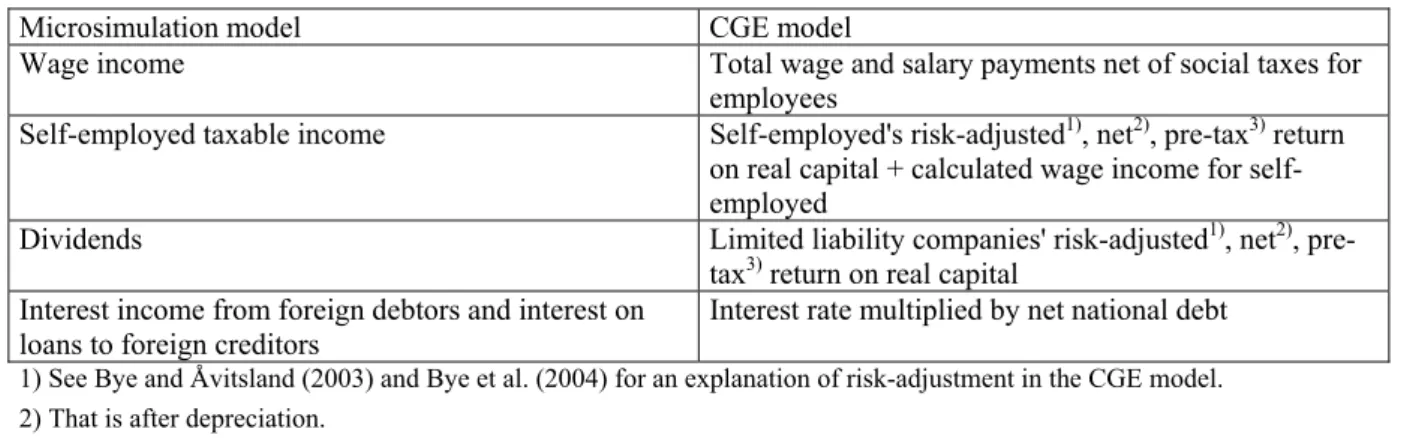
variables as exogenous input into the microsimulation model13. Broadly speaking, we have linked incomes in the microsimulation and CGE models as shown in table 1. The numerical changes from the CGE analyses are shown in appendix A.
Table 1. Linking incomes in the microsimulation and CGE models
Microsimulation model CGE model
Wage income Total wage and salary payments net of social taxes for
employees
Self-employed taxable income Self-employed's risk-adjusted1), net2), pre-tax3) return
on real capital + calculated wage income for self-employed
Dividends Limited liability companies' risk-adjusted1), net2),
pre-tax3) return on real capital
Interest income from foreign debtors and interest on loans to foreign creditors
Interest rate multiplied by net national debt
1) See Bye and Åvitsland (2003) and Bye et al. (2004) for an explanation of risk-adjustment in the CGE model. 2) That is after depreciation.
3) But after paying of VAT and/or investment tax on material inputs and investment goods.
13 In our CGE simulations, public sector's net savings and net wealth are unchanged from baseline scenario to policy
alternative. This implies that changes in net national savings and net wealth are equal to the private sector's change in these variables.
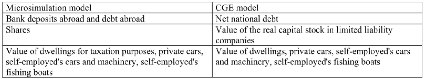
We have linked wealth in the microsimulation and CGE models as shown in table 2. The numerical changes from the CGE model are reported in appendix A.
Table 2. Linking wealth in the microsimulation and CGE models
Microsimulation model CGE model
Bank deposits abroad and debt abroad Net national debt
Shares Value of the real capital stock in limited liability
companies Value of dwellings for taxation purposes, private cars,
self-employed's cars and machinery, self-employed's fishing boats
Value of dwellings, private cars, self-employed's cars and machinery, self-employed's fishing boats
In addition, expenses and some components of income and wealth in the microsimulation model are absent in the CGE model. We have chosen to keep these variables constant, including interest income from Norwegian debtors, interest on loans to Norwegian creditors14, domestic bank deposits and domestic debt.
A detailed description of assumptions and the linking of income and wealth in the two models are given in appendix B.1 and B.2.
4.3 Transfers
In the CGE model, the different transfers, that is pensions, sickness benefits, unemployment benefits, child benefits, other transfers from Central Government and other transfers from Local Government, automatically change as a result of changes in the wage rate, total wage payments or the price index of aggregate private consumption. The detailed linking of transfers in the two models is reported in appendix B.3. The numerical changes in transfers from the CGE analyses are reported in appendix A.
14 The pre-tax income concept used in the microsimulation model includes interest income but excludes interest on debt.
Stipulated capital income stemming from housing is also excluded. Dwelling services are part of private consumption expenditure.
4.4 Leisure and savings
Leisure
Leisure is part of the utility function in the CGE model, but not in the microsimulation model. Higher (lower) incomes due to increased (lower) labour supply are fed into the microsimulation model but the corresponding decrease (increase) in leisure is not taken into account. Therefore, only the positive (negative) aspects of increased (decreased) labour supply are included in the microsimulation model.
Savings
There is a somewhat analogous problem concerning savings: In steady state, net savings in real capital are zero, but real capital wealth may have increased (decreased) from baseline scenario to a policy alternative due to positive (negative) savings in real capital earlier in the path. We employ changes in income and wealth from the CGE model's steady state when linking the microsimulation and CGE model. This means that only the gains (losses) from increased (decreased) savings in real capital are taken into account when we link the two models. A similar argument applies to financial savings.
4.5 Evaluation of the linking procedure
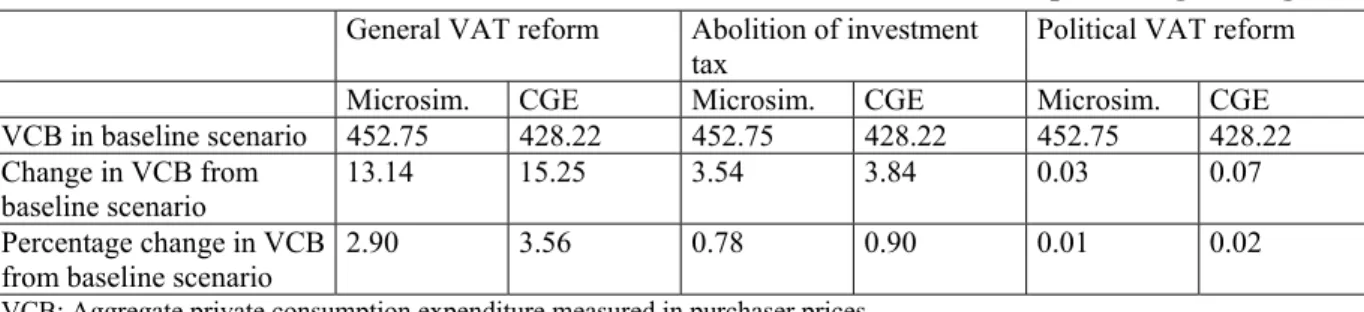
In order to evaluate our sequential linking procedure, we compare aggregate private consumption expenditure in current prices in the two models. Both the level in the baseline scenario and the change and percentage change from baseline scenario to the three policy alternatives are compared, see table 3.
Table 3. Aggregate private consumption expenditure. Current purchaser prices.
Microsimulation results versus CGE results. Billion NOK and percentage change General VAT reform Abolition of investment
tax Political VAT reform
Microsim. CGE Microsim. CGE Microsim. CGE
VCB in baseline scenario 452.75 428.22 452.75 428.22 452.75 428.22
Change in VCB from baseline scenario
13.14 15.25 3.54 3.84 0.03 0.07 Percentage change in VCB
from baseline scenario 2.90 3.56 0.78 0.90 0.01 0.02
VCB: Aggregate private consumption expenditure measured in purchaser prices.
Numbers from the baseline scenario apply to the year 1995 in the microsimulation model, while these numbers apply to the steady state in the CGE model. The steady state numbers may, as mentioned earlier, be interpreted as representing the economy in 1995 after it has "calmed down".
Concerning evaluation of our linking procedure, the impression is that it gives quite reasonable results. There is not complete consistency, visualized by the fact that the change in aggregate private
consumption expenditure is not identical in the two models. The differences between the results from the CGE and microsimulation models are not significant, however, cf. footnote 18.
5. Results
The distribution of the standard of living over a population can be summarised in several ways. In this paper, we focus on the simple aggregated measure equality (E), defined as (1 - G), where G is the Gini-coefficient15. The equality measure varies between 0 and 1, and the value increases when the distribution of the standard of living becomes more equal.
It is difficult to grasp whether a change in the degree of equality is large or not. We therefore
"translate" a change in the degree of equality into a change in the standard of living per person, while
15 The Gini-coefficient is the most common measure of inequality in the economic literature, see Aaberge (2001) for an
simultaneously keeping Sen welfare constant. Sen welfare is defined as: S = WE, where S is Sen welfare, W is average standard of living per person and E is the degree of equality, cf. Sen (1974) for an axiomatic basis. The average standard of living per person, W, is in this paper measured by the real consumption expenditure per equivalent adult, taken from the microsimulation model in 1995 and E is defined as above. When Sen welfare is to be unchanged from baseline scenario to the three policy alternatives, a reforms' increase (decrease) in equality must be compensated by a decrease (increase) in the standard of living per person. Appendix C may be consulted for details.
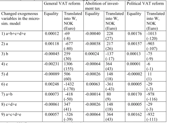
Table 4 shows the absolute change in the degree of equality from baseline scenario to the three policy alternatives for our main simulation, 1), and for different decompositions, 2) - 9). It also shows the change in the degree of equality "translated" into a change in the standard of living per person for given Sen welfare. All these numbers show that the interaction effect is close to 0, i.e. the sum of single-effects is almost identical to the effect of changing these variables simultaneously16.
Our main simulation, which is the case where all CGE effects are taken into account, (cf. 1) in table 4) shows that equality is clearly increased with the political VAT reform. With the general VAT reform the change in equality are close to 0. Abolition of the investment tax implies a small reduction in equality, but the effect is quite close to zero17,18.
16 One exception is the general VAT reform where summing the equality effects of c, d and e, respectively, (cf. 4), 5) and 6)
in table 4) is equal to 0.00072, while the effect on equality of changing the relevant variables simultaneously is equal to -0.00061 (cf. 8) in table 4).
17 All of these conclusions hold when we perform sensitivity analyses with respect to the choice of equivalence scale (cf.
footnote 8).
18 Since our linking procedure does not ensure complete consistency, visualized by the fact that the change in aggregate
private consumption expenditure is not identical in the two models, we have undertaken the following exercise: The main simulation of the general VAT reform (cf. 1) in table 4) is undertaken while simultaneously changing proportionally all incomes, wealth and transfers so that the resulting percentage change in aggregate private consumption expenditure in the microsimulation model is identical with the percentage change in the CGE model. The result shows that the change in equality is still close to 0 (-0.00005).
Table 4. Absolute change in the degree of equality from baseline scenario, for three
policy reforms and for different decompositions. Translation of this into an absolute change in NOK (Euro1)) in the standard of living per person (W2)) for given Sen welfare.
General VAT reform Abolition of
invest-ment tax Political VAT reform Changed exogeneous
variables in the micro-sim. model Equality Translated into W, NOK (Euro) Equality Translated into W, NOK (Euro) Equality Translated into W, NOK (Euro) 1) a+b+c+d+e 0.00012 -69 (-8) -0.00040 (27) 228 0.00176 -1013 (-120) 2) a 0.00118 -677 (-80) -0.00038 217 (26) 0.00157 -903 (-107) 3) b -0.00045 259 (30) 0.00024 -137 (-17) 0.00013 -75 (-9) 4) c -0.00231 1306 (155) -0.00064 364 (43) 0.00001 -6 (-1) 5) d -0.00089 506 (60) -0.00026 (18) 148 -0.00002 (1) 11 6) e 0.00248 -1432 (-170) 0.00063 -361 (-43) 0.00005 -29 (-3) 7) a+b 0.00073 -418 (-50) -0.00014 (9) 80 0.00170 -978 (-116) 8) c+d+e -0.00061 347 (41) -0.00026 (18) 148 0.00005 -29 (-3) 9) a+c+d+e 0.00057 -326 (-39) -0.00064 (43) 364 0.00162 -932 (-111)
a: changed VAT rates on consumer goods and services b: changed producer prices from the CGE simulations
c: changed pre-tax incomes, excl. of dividends (and transfers), and changed pre-tax wealth from the CGE simulations d: changed pre-tax dividends from the CGE simulations
e: changed pre-tax transfers from the CGE simulations
______________________________________________________________________________________ 1) The exchange rate used in the calculations is equal to 8.42 NOK per Euro.
2) W is equal to 130491 NOK (15498 Euro) in 1995.
When we undertake a "traditional" simulation of the microsimulation model, i.e. only changing the VAT rates (cf. 2) in table 4), the results for the political VAT reform and abolition of the investment tax are still respectively a clear increase and a small decrease in equality, where the latter is still quite close to zero. The inclusion of general equilibrium effects does not change the results, in other words. For the political VAT reform, the main explanation of the equality result in both cases seems to be the halving of the VAT rate on food and non-alcoholic beverages. This halving, together with the fact that persons with a low standard of living generally have a larger budget share of food than persons with a high standard of living, implies increased equality. With abolition of the investment tax the reason for
the small decrease in equality when general equilibrium effects are not taken into account, is the increase in the VAT rate on goods19. This increase, together with the fact that persons with a low standard of living generally have a larger budget share of goods, as opposed to services, than persons with a high standard of living, implies reduced equality.
However, with the general VAT reform, the inclusion of general equilibrium effects is important for the results. For this reform, equality is increased when CGE effects are not taken into account as opposed to almost unchanged equality when such effects are included. Increased equality when general equilibrium effects are not included can be explained by introduction of VAT on more services. This, together with the fact that persons with a low standard of living generally have a smaller budget share of services than persons with a high standard of living, results in increased equality.
Which components from the general equilibrium analysis contribute to change the result from an increase in equality to a zero effect on equality? Answers can be found in rows 3-9 of table 4. We see that taking account of changed producer prices (b), changed pre-tax incomes, exclusive of dividends, and changed wealth (c), and changed dividends (d) contribute to reduced equality. On the other hand, changed pre-tax transfers (e) contribute to increased equality. The effect on equality of the former changes (i.e. b, c, and d) outweighs the effect on equality of the latter change (i.e. e), resulting in the stated overall zero effect on equality instead of increased equality.
Explanations of the partial effects above are as follows: Pre-tax incomes, exclusive of dividends, (where wage income is a major component) increase in the CGE simulations. This, taken together with the fact that wage income generally constitutes a smaller share of income for persons with a low
19 Remember that a public revenue neutral increase in the VAT rate on goods and some services is part of the reform that
standard of living than for persons with a high standard of living, explains the reduction in equality. Dividends are increased in the CGE simulations, implying reduced equality since dividends generally constitute a smaller share of income for persons with a low standard of living than for persons with a high standard of living. In the CGE model many transfers depend upon wages (wage indexation). Since wages are increased in the CGE simulations, transfers are then automatically also increased, and equality increases because transfers generally constitute a larger share of income for persons with a low standard of living than for persons with a high standard of living.
A point worth stressing is the importance of including general equilibrium changes in all the main income components and transfers. For example, with the general VAT reform only including changes in pre-tax incomes, excl. of dividends, and pre-tax wealth together with changed producer prices would have resulted in a clear decrease in equality (the sum of 4) and 7) in table 4 is equal to -0.00158). This is in sharp contrast to almost unchanged equality when also general equilibrium changes in pre-tax dividends and pre-tax transfers are included. Robilliard et al. (2001) do not take into account changes in non-labour income (like transfers and dividends).
Table 4 also provides a decomposition of the effects on equality of abolition of the investment tax. Taking into account changes in producer prices (b) increases equality, but this is offset by the negative effect of increased dividends (d). Increased pre-tax incomes, exclusive of dividends, and changed wealth (c) contribute substantially to decreased equality, but this is offset by the effect of increased transfers (e). Thus in this policy reform the different "general equilibrium effects", cancel each other out, implying that the effect on equality is the same in the full analysis (cf. 1) in table 4) and the simple approach (cf. 2) in table 4). However, the sizes of the partial equilibrium effects are relatively important, and neglecting effects from e.g. transfers would have given a substantially more negative effect on equality of this policy reform.
Table 4 also shows the detailed decomposition of the effects on equality from the political VAT reform. We notice that the inclusion of general equilibrium effects is of no importance concerning the equality results. This is due to small changes in the variables from the CGE analysis, cf. table A.1. - A.5. in appendix A.
6. Concluding remarks
In this paper we have used a microsimulation model of the Norwegian economy subsequent to a CGE model to analyse effects on the degree of equality of three indirect taxation reforms. Efficiency effects of these three reforms have earlier been analysed by Bye et al. (2004) by employing a CGE model with one representative consumer.
Consumer prices, pre-tax nominal incomes, wealth and transfers are all exogenous in the
microsimulation model and percentage changes in such variables from the CGE anlyses are fed into the microsimulation model. By combining CGE and microsimulation models in such a way, the equality analyses are enriched by taking into account potentially important information from the general equilibrium analyses.
The three reforms analysed in this paper are evaluated against a baseline scenario which describes the Norwegian, non-uniform, system of indirect taxation in 1995. The first reform analysed is the general VAT reform, where all goods and services are subject to the same VAT rate. The second reform analysed is abolition of the investment tax, where the investment tax is set equal to zero. This reform is both analysed separately and as part of the general VAT reform. The third reform analysed is the political VAT reform. This reform introduces another non-uniform VAT system, of which a main characteristic is the halving of the VAT rate on food and non-alcoholic beverages. This VAT system
was actually implemented in Norway in 2001. All the three reforms are in the CGE analysis made public revenue neutral by changes in the VAT rate20.
We find that equality is clearly increased with the political VAT reform. Concerning the general VAT reform and abolition of the investment tax the changes in equality are close to 0. When general equilibrium effects are not taken into account, the equality results survive with the political VAT reform and abolition of the investment tax. This is not the case with the general VAT reform, where the zero effect on equality is turned into an increase in equality. Both the inclusion of changed producer prices and changed pre-tax nominal incomes, wealth and transfers contribute to this alteration of the equality result.
A priori the only case where the inclusion of general equilibrium effects is irrelevant to the overall equality results, is the one where these effects are small. The political VAT reform is an example of such a case, as pointed out above. In all other cases a microsimulation analysis with the inclusion of general equilibrium effects will have to be carried out in order to know how these effects influence the equality results. With the general VAT reform the inclusion of general equilibrium effects changes the equality result substantially, while with abolition of the investment tax the different general
equilibrium effects cancels each other out.
Another finding is the importance of including general equilibrium changes in all the main income components and transfers. For example, with the general VAT reform only including changes in pre-tax incomes, excl. of dividends, and pre-pre-tax wealth together with changed producer prices would have resulted in a clear decrease in equality. This is in sharp contrast to unchanged equality when also
20 Bye et al. (2004) find that welfare is increased with the general VAT reform, while it is reduced with the other two
general equilibrium changes in pre-tax dividends and pre-tax transfers are included. Robilliard et al. (2001) do not take into account changes in non-labour income (like transfers and dividends).
References
Aaberge, R. (2001): Axiomatic characterization of the Gini coefficient and Lorenz curve orderings, Journal of Economic Theory 101, 115-132.
Aaberge, R., U. Colombino, E. Holmøy, B. Strøm and T. Wennemo (2004): Population ageing and fiscal sustainability: An integrated micro-macro analysis of required tax changes, Discussion Paper 367, Statistics Norway.
Aasness, J. (1995): A microsimulation model of consumer behavior for tax analyses, Paper presented at the Nordic seminar on microsimulation models, Oslo, May 1995.
Aasness, J. (1997): "Effects on poverty, inequality and welfare of child benefit and food subsidies» in N. Keilman, J. Lyngstad, H. Bojer, and I. Thomsen (eds): Poverty and economic inequality in industrialized western countries, Oslo: Scandinavian University Press, 123-140.
Aasness, J., A. Benedictow and M. F. Hussein (2002): Distributional efficiency of direct and indirect taxes, Rapport 69, Economic Research Programme on Taxation, Oslo: Norges Forskningsråd.
Aasness, J, T. Bye, and H. T. Mysen (1996): Welfare effects of emission taxes in Norway, Energy Economics 18, 335-346.
Aasness, J., E. Fjærli, H. A. Gravningsmyhr, A. M. K. Holmøy and Bård Lian (1995): The Norwegian microsimulation model LOTTE: Applications to personal and corporate taxes and social security benefits, DAE Working Papers no 9533, Microsimulation Unit, Department of Applied Economics, University of Cambridge.
Aasness, J. and B. Holtsmark (1993): Consumer demand in a general equilibrium model for environmental analysis, Discussion Paper 105, Statistics Norway.
Atkinson, A.B. (1992): Measuring poverty and differences in family composition, Economica 59, 1-16.
Blackorby, C. and D. Donaldson (1993): Adult-equivalence scales and the economic implementation of interpersonal comparisons of well-being, Social Choice and Welfare 10, 335-61.
Bojer, H. (1977): The effects on consumption of household size and composition, European Economic Review 9, 169-193.
Bourguignon, F., A.-S. Robilliard and S. Robinson (2005): "Representative versus Real Households in the Macroeconomic Modeling of Inequality", in Kehoe, T. J., T. N. Srinivasan and J. Whalley (eds.) Frontiers in Applied General Equilibrium Modeling, Cambridge University Press, 219-254.
Bourguignon, F. and A. Spadaro (2005): Microsimulation as a Tool for Evaluating Redistribution Policies, unpublished Working Paper, Paris-Jourdan Sciences Economiques. The paper can be downloaded at the Web address: http://www.pse.ens.fr/document/wp200502.pdf
Bowitz, E. and Å. Cappelen (2001): Modeling income policies: some Norwegian experiences 1973-1993, Economic Modelling 18, 349-379.
Buhman, B., L. Rainwater, G. Schmaus, and T.M. Smeeding (1988), Equivalence scales, well-being, inequality, and poverty: sensitivity estimates across ten countries using the Luxembourg Income Study (LIS) database, Review of Income and Wealth 34, 115-142.
Bye, B. (2000): Environmental tax reform and producer foresight: An intertemporal computable general equilibrium analysis, Journal of Policy Modeling 22 (6), 719-752.
Bye, B. (2003): Consumer behaviour in the MSG-6 model - a revised version, Manuscript, Statistics Norway.
Bye, B., B. Strøm and T. Åvitsland (2004): Welfare effects of VAT reforms: A general equilibrium analysis, Manuscript, Revised version of Discussion Paper 343, Oslo: Statistics Norway.
Bye, B. and T. Åvitsland (2003): The welfare effects of housing taxation in a distorted economy: A general equilibrium analysis, Economic Modelling 20(5), 895-921.
Davies, J. B. (2004): Microsimulation, CGE and Macro Modelling for Transition and Developing Economies, Discussion Paper No. 2004/08, United Nations University - World Institute for Development Economics Research.
Davies, J., F. St-Hilaire and J. Whalley (1984): Some Calculations of Lifetime Tax Incidence, American Economic Review, 74 (4), 633-649.
Epland, J. and G. Frøiland (2002): Husholdningenes inntekter: En sammenlikning av nasjonalregnskapet og inntektsundersøkelsens inntektsbegreper, Notater 2002/76, Statistisk sentralbyrå.
Essama-Nssah, B. (2005): The Poverty and Distributional Impact of Macroeconomic Shocks and Policies: A Review of Modeling Approaches, Policy Research Working Paper 3682, World Bank, Washington, DC.
Fæhn, T. and E. Holmøy (2000): "Welfare effect of trade liberalisation in distorted economies: A dynamic general equilibrium assessment for Norway". In Harrison, G. W. et al. (eds): Using dynamic general equilibrium models for policy analysis, North-Holland, Amsterdam.
Herigstad, H. (1979): Forbrukseiningar, Rapporter 79/16, Statistisk sentralbyrå.
Holmøy, E., and T. Hægeland (1997): Aggregate Productivity Effects and Technology Shocks in a Model of Heterogeneous Firms: The Importance of Equilibrium Adjustments, Discussion Paper 198, Oslo: Statistics Norway.
Holmøy, E., G. Nordén, and B. Strøm (1994): MSG-5, A complete description of the system of equations, Rapporter 94/19, Oslo: Statistics Norway.
Klette, T. J. (1994): Estimating price-cost margins and scale economies from a panel of micro data, Discussion Papers 130, Oslo: Statistics Norway.
Nelson, J. (1993): Household equivalence scales: theory versus policy? Journal of Labor Economics 11, 471-493.
Robilliard, A.-S., F. Bourguignon and S. Robinson (2001): Crisis and Income Distribution: A Micro-Macro Model for Indonesia, mimeo. The paper can be downloaded at the Web address:
http://www.economie.uqam.ca/PDF/bourguignon.doc
Røed Larsen, E. and J. Aasness (1996): Kostnader ved barn og ekvivalensskalaer basert på Engels metode og forbruksundersøkelsen 1989-91, Offentlige overføringer til barnefamilier, NOU 1996:13, Oslo: Akademika, 305-317.
Savard, L. (2005): Poverty and Inequality Analysis within a CGE Framework: A Comparative
Analysis of the Representative Agent and Microsimulation Approaches, Development Policy Review,
23 (3), 313-331.
Sen, A. (1974): Informational bases of alternative welfare approaches: aggregation and income distribution, Journal of Public Economics 4, 387-403.
Wold, I. S. (1998): Modellering av husholdningenes transportkonsum for en analyse av grønne skatter: Muligheter og problemer innenfor rammen av en nyttetremodell, Notater 98/98, Statistisk sentralbyrå.
Appendix A
Simulated changes in consumer prices, income, wealth and
transfers
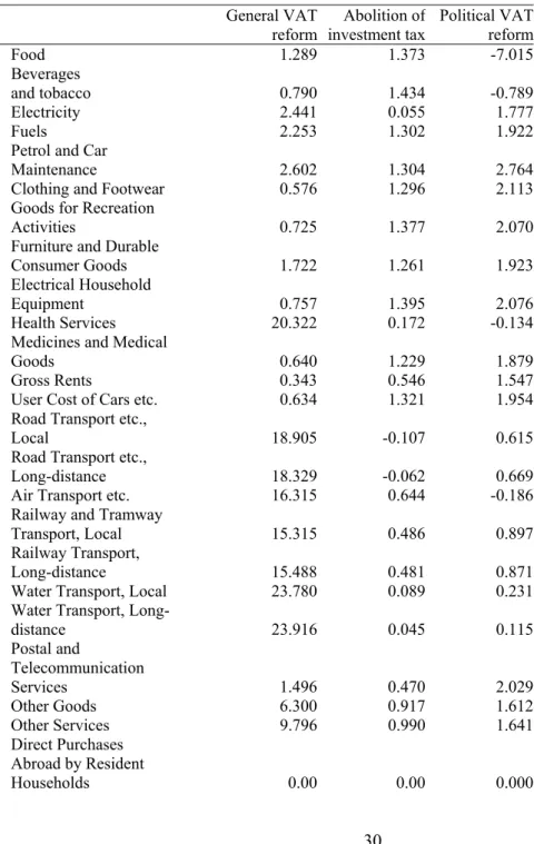
Table A.1. Consumer prices when producer prices are endogenous. Percentage changes from baseline scenario. Long run effects
General VAT
reform investment taxAbolition of Political VAT reform
Food 1.289 1.373 -7.015
Beverages
and tobacco 0.790 1.434 -0.789
Electricity 2.441 0.055 1.777
Fuels 2.253 1.302 1.922
Petrol and Car
Maintenance 2.602 1.304 2.764
Clothing and Footwear 0.576 1.296 2.113
Goods for Recreation
Activities 0.725 1.377 2.070
Furniture and Durable
Consumer Goods 1.722 1.261 1.923
Electrical Household
Equipment 0.757 1.395 2.076
Health Services 20.322 0.172 -0.134
Medicines and Medical
Goods 0.640 1.229 1.879
Gross Rents 0.343 0.546 1.547
User Cost of Cars etc. 0.634 1.321 1.954
Road Transport etc.,
Local 18.905 -0.107 0.615
Road Transport etc.,
Long-distance 18.329 -0.062 0.669
Air Transport etc. 16.315 0.644 -0.186
Railway and Tramway
Transport, Local 15.315 0.486 0.897
Railway Transport,
Long-distance 15.488 0.481 0.871
Water Transport, Local 23.780 0.089 0.231
Water Transport, Long-
distance 23.916 0.045 0.115 Postal and Telecommunication Services 1.496 0.470 2.029 Other Goods 6.300 0.917 1.612 Other Services 9.796 0.990 1.641 Direct Purchases Abroad by Resident Households 0.00 0.00 0.000
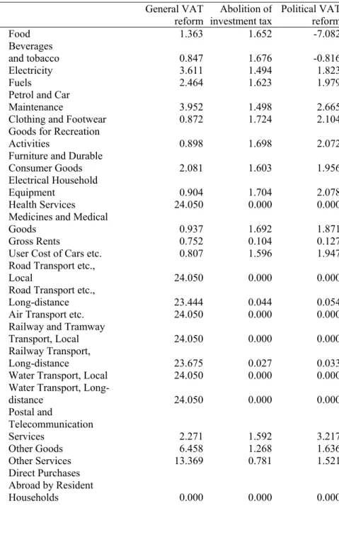
Table A.2. Consumer prices when producer prices are constant. Percentage changes from baseline scenario. Long run effects
General VAT
reform investment taxAbolition of Political VAT reform
Food 1.363 1.652 -7.082
Beverages
and tobacco 0.847 1.676 -0.816
Electricity 3.611 1.494 1.823
Fuels 2.464 1.623 1.979
Petrol and Car
Maintenance 3.952 1.498 2.665
Clothing and Footwear 0.872 1.724 2.104
Goods for Recreation
Activities 0.898 1.698 2.072
Furniture and Durable
Consumer Goods 2.081 1.603 1.956
Electrical Household
Equipment 0.904 1.704 2.078
Health Services 24.050 0.000 0.000
Medicines and Medical
Goods 0.937 1.692 1.871
Gross Rents 0.752 0.104 0.127
User Cost of Cars etc. 0.807 1.596 1.947
Road Transport etc.,
Local 24.050 0.000 0.000
Road Transport etc.,
Long-distance 23.444 0.044 0.054
Air Transport etc. 24.050 0.000 0.000
Railway and Tramway
Transport, Local 24.050 0.000 0.000
Railway Transport,
Long-distance 23.675 0.027 0.033
Water Transport, Local 24.050 0.000 0.000
Water Transport, Long-
distance 24.050 0.000 0.000 Postal and Telecommunication Services 2.271 1.592 3.217 Other Goods 6.458 1.268 1.636 Other Services 13.369 0.781 1.521 Direct Purchases Abroad by Resident Households 0.000 0.000 0.000
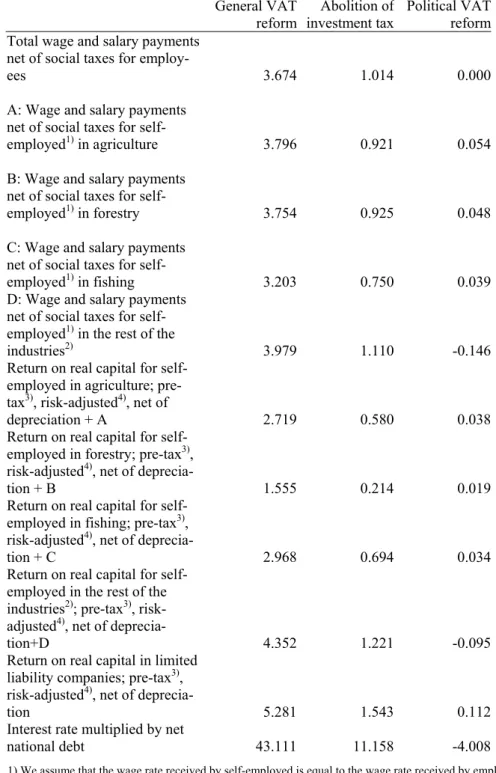
Table A.3. Nominal incomes. Percentage changes from baseline scenario. Long run effects
General VAT
reform investment taxAbolition of Political VAT reform Total wage and salary payments
net of social taxes for
employ-ees 3.674 1.014 0.000
A: Wage and salary payments net of social taxes for
self-employed1) in agriculture 3.796 0.921 0.054
B: Wage and salary payments net of social taxes for
self-employed1) in forestry 3.754 0.925 0.048
C: Wage and salary payments net of social taxes for
self-employed1) in fishing 3.203 0.750 0.039
D: Wage and salary payments net of social taxes for self-employed1) in the rest of the
industries2) 3.979 1.110 -0.146
Return on real capital for self-employed in agriculture; pre-tax3), risk-adjusted4), net of
depreciation + A 2.719 0.580 0.038
Return on real capital for self-employed in forestry; pre-tax3),
risk-adjusted4), net of
deprecia-tion + B 1.555 0.214 0.019
Return on real capital for self-employed in fishing; pre-tax3),
risk-adjusted4), net of
deprecia-tion + C 2.968 0.694 0.034
Return on real capital for self-employed in the rest of the industries2); pre-tax3),
risk-adjusted4), net of
deprecia-tion+D 4.352 1.221 -0.095
Return on real capital in limited liability companies; pre-tax3),
risk-adjusted4), net of
deprecia-tion 5.281 1.543 0.112
Interest rate multiplied by net
national debt 43.111 11.158 -4.008
1) We assume that the wage rate received by self-employed is equal to the wage rate received by employees.
2) That is all private production sectors, with the exception of agriculture, forestry, fishing, dwelling services, production of electricity, oil and gas exploration and drilling, production and pipeline transport of oil and gas, ocean transport and imputed service charges from financial institutions.
3) But after paying of VAT and/or investment tax.
4) See Bye and Åvitsland (2003) and Bye et al. (2004) for an explanation of risk-adjustment in the CGE model.
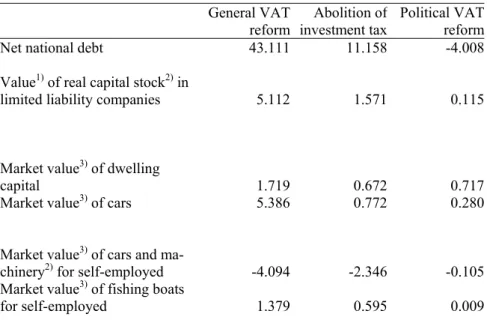
Table A.4. Nominal wealth. Percentage changes from baseline scenario. Long run effects
General VAT
reform investment taxAbolition of Political VAT reform
Net national debt 43.111 11.158 -4.008
Value1) of real capital stock2) in
limited liability companies 5.112 1.571 0.115
Market value3) of dwelling
capital 1.719 0.672 0.717
Market value3) of cars 5.386 0.772 0.280
Market value3) of cars and
ma-chinery2) for self-employed -4.094 -2.346 -0.105
Market value3) of fishing boats
for self-employed 1.379 0.595 0.009
1) Measured in purchaser price indexes, exclusive of VAT and/or the investment tax.
2) Comprising all private production sectors, with the exception of dwelling services, production of electricity, oil and gas exploration and drilling, production and pipeline transport of oil and gas, ocean transport and imputed service charges from financial institutions. 3) Measured in purchaser price indexes, inclusive of VAT and/or the investment tax.
Table A.5. Transfers. Percentage changes from baseline scenario. Long run effects
General VAT
reform investment taxAbolition of Political VAT reform
Pension 3.821 0.943 0.067
Sickness benefits etc. 3.674 1.014 0.000
Unemployment benefits 3.674 1.014 0.000
Child benefits 3.821 0.943 0.067
Other transfers, Central
Gov-ernment 3.821 0.943 0.067
Other transfers, Local
Appendix B
The symbol and name of the microsimulation variables (MSV) are first mentioned. Next, the symbol and name of the corresponding CGE variables (CGEV) are written down. This means that all microsimulation variables under the heading 1) MSV are exogenously changed by the percentage change in the variable under the heading 1) CGEV, and so forth. Assumptions made are then clarified, together with other comments. B.1 deals with income variables, B.2 with wealth variables and B.3 with transfer variables.
B.1 Combining income variables in the CGE and microsimulation
models
1) MSV
K2101, wage income and unemployment benefits for employees
K21013, of this: wage income only into the basis for calculation of member's premium to the National Insurance Scheme
K2102, income entitled to the seaman's deduction
K2103, income stemming from child care in one's own home K2104, profit from payments in kind
K2105, other income stemming from labour
K2401, children's wage income (children under 13 years of age)
K1607, calculated personal income limited liability company, liberal occupation K1608, calculated personal income limited liability company, other industry
K3212, contribution to private/public Norwegian pension scheme in connection with the employment XEKSTRA, adjustment of personal income
XELF, own wages in an enterprise XGLF, basis for deduction of wages XKAG, basis for return to capital
XKN, corrected self-employed, taxable income XLAKT, wage costs concerning active owners
1) CGEV
yww, total wage and salary payments net of social taxes
2) MSV
K1601, calculated personal income one-man enterprise, primary industry K1604, calculated personal income partner-assessed company, primary industry
K1612, part of wage income/pension stemming from enterprise from which the person in question receives calculated personal income, primary industry
K1701, remuneration for work to partner in partner-assessed company where personal income is not calculated, primary industry
2) CGEV 13 13 12 12 11 11ls ww ls ww ls ww + +
wwj is wage per hour to wage earners in production sector j in current prices and net of social taxes, lsj is number of hours worked by self-employed in production sector j, j = 11 (agriculture), 12 (forestry) and 13 (fishing).
3) MSV
K1602, calculated personal income one-man enterprise, liberal occupation K1605, calculated personal income partner-assessed company, liberal occupation
K1613, part of wage income/pension stemming from enterprise from which the person in question receives calculated personal income, liberal occupation
3) CGEV
85 85ls
ww
85 is the industry other private services.
4) MSV
K1603, calculated personal income one-man enterprise, other industry K1606, calculated personal income partner-assessed company, other industry
K1614, part of wage income/pension stemming from enterprise from which the person in question receives calculated personal income, other industry
K1702, remuneration for work to partner in partner-assessed company where personal income is not calculated, other industry
4) CGEV {
∑
} ∈PP\PW,11,12,13,85 j j jls wwPP is all private production sectors and PW is the private production sectors 71 (Production of electricity), 68 (Oil and gas exploration and drilling), 64 (Production and pipeline transport of oil and gas), 60 (Ocean transport), 83 (Dwelling services) and 89 (Imputed service charges from financial institutions).
5) MSV
5) CGEV 11 11 50 , 40 , 10 11 , 11 , 11 , 11 (bp ˆ risk)pjbk ww ls sse i i i i i − − +
∑
= δsse11 is the share of self-employed in agriculture, i = 10, 40 and 50 are respectively buildings, cars and machinery, bpi,11 is the user cost of capital type i per NOK invested in agriculture, δˆi,11 is the
depreciation rate of capital type i in agriculture, risk is the risk premium, pjbi is the purchaser price index, exclusive of VAT and the investment tax, for new investment, capital type i and ki,11 is the capital stock of type i in agriculture in constant prices.
6) MSV
K2702, self-employed, taxable income, forestry
6) CGEV 12 12 50 , 40 , 10 12 , 12 , 12 , 12 (bp ˆ risk)pjbk ww ls sse i i i i i
∑
= + − −δ 7) MSVK2703, self-employed, taxable income, fishing
7) CGEV 13 13 50 , 30 13 , 13 , 13 , 13 (bp ˆ risk)pjbk ww ls sse i i i i i
∑
= + − −δ30 is the capital type ships and fishing boats.
8) MSV
K2704, other self-employed, taxable income (inclusive of liberal occupation) K27041, self-employed, taxable income, partnership company
8) CGEV {
∑
}∑
∈ {∑
} ∈ = + − − 13 , 12 , 11 , \ 13 , 12 , 11 , \ 10,40,50,30,80 , , , ˆ ) ( PW PP j j j PW PP j i j i i j i j i j bp risk pjbk ww ls sse δ80 is the capital type aircraft.
There is a clear coherence between income types 2) to 8) since self-employed, taxable income both consists of capital income and the self-employed's labour income and calculated personal income is meant to reflect the self-employed's labour income. The above expressions for the self-employed's labour income part of self-employed, taxable income and for the calculated personal income are therefore identical. We assume that the self-employed's wage rate is equal to the wage rate received by employees.
All private production sectors with the exception of 71 (Production of electricity), 68 (Oil and gas exploration and drilling), 64 (Production and pipeline transport of oil and gas), 60 (Ocean transport), 83 (Dwelling services) and 89 (Imputed service charges from financial institutions) are included in the above calculations. 68 (Oil and gas exploration and drilling), 64 (Production and pipeline transport of oil and gas) and 60 (Ocean transport) are excluded because of a constant real capital stock and no user costs of real capital attached to them. 89 (Imputed service charges from financial institutions) are not included since there is no real capital stock there. 83 (Dwelling Services) are excluded since this is an artificially constructed private production sector directly attached to private consumption. We have chosen to omit 71 (Production of electricity) since the user cost of capital in this industry differs conceptually from the other user costs and since real capital is "almost exogenous".
Concerning item 5) to 8), we use the net return on real capital for self-employed as an approximation to the self-employed's capital income part of self-employed, taxable income. The net return in these
expressions is generally before paying of taxes. An exception is paying of the VAT and the investment tax since we employ the purchaser price index of new investments exclusive of VAT and the
investment tax. We then think of the difference between the net return on real capital employing respectively the purchaser price index inclusive and exclusive of the VAT and the investment tax as representing the paying of these two taxes. Since the microsimulation model only deals with personal taxes the VAT and the investment tax on inputs are not part of this model.
Gross production in agriculture, forestry and fishing is exogenous in the CGE model. Therefore changes in employment and real capital may only take place through substitution effects, and not through scale effects.
In the microsimulation model, the calculated personal income is either exogenous, as in item 2) to 4), or computed by means of individual variables, as in item 1) (the variables starting with the letter X). The former constitutes the largest part. For practical reasons, we assume that all the "X-variables" in 1), even though they are divided into the two categories primary industry and other industry, are changed by the change in employees' wage income. The self-employed's endogenous calculated personal income will then change by roughly the same percentage.
9) MSV
K3104, dividends from shares giving the right to refundment K31041, of this: dividends from funds of shares
9) CGEV { }