layer instability and tonal noise of an
airfoil at Reynolds number 150,000
Reprints and permission:
sagepub.co.uk/journalsPermissions.nav DOI: 10.1177/ToBeAssigned www.sagepub.com/
Marlene Sanjose
1, Aaron Towne
2, Prateek Jaiswal
1, Stephane Moreau
1, Sanjiva Lele
2,
Adrien Mann
3Abstract
A direct numerical simulation of the flow field around a controlled-diffusion airfoil within an anechoic wind-tunnel at5◦ incidence and a high Reynolds number of1.5×105 is performed for the first time using a Lattice Boltzmann Method. The simulation compares favorably with experimental measurements of wall-pressure, wake statistics, and far-field sound. The simulation noticeably captures experimentally observed high-amplitude acoustic tones that rise above a broadband hump. Both noise components are related to a breathing of a recirculation bubble formed around 65-70% of the chord, and to Kelvin-Helmholtz instabilities in the separated shear layer that yield rollers that break down into turbulent vortices whose diffraction at the trailing edge produces a strong dipole acoustic field. A wavelet analysis of the wall-pressure signals combined with some flow visualization has shown that the flow statistics are dominated by intense events caused by intermittent, large and intense bursting rollers. Several modal analyses of these events are performed on both the wall pressure fluctuations and the span averaged flow field in order to analyse the boundary layer instability which triggers the typical sharp tones over a broadband hump in airfoil noise. A suction side Kelvin-Helmholtz instability is observed to be coupled with a pressure side vortex shedding induced by the sudden transition to turbulence and the blunt trailing edge.
Keywords
Aeroacoustic, Tonal noise, Boundary layer instability, Turbomachinery, Ventilation Systems
Introduction
Airfoil self-noise can be seen as the canonical aeroacoustic problem for wall-bounded flows and is directly related to the minimum noise generated by a fixed wing or a rotating machine. It is usually produced by the scattering of boundary-layer vortical disturbances into acoustic waves at the airfoil trailing edge. This process typically produces a broadband acoustic signature, as seen, for instance, in the turbulent flow regime (8◦ geometrical angle-of-attack) over a cambered thin Controlled-Diffusion (CD) airfoil, characteristic of modern low-speed and high-speed fan blade design. Such a flow regime has been extensively studied both experimentally1–5 and numerically6–10. In addition to this broadband behavior, sharp tones that rise above the broadband noise spectrum have also been experimentally observed for the same airfoil for certain flow configurations1,5.
Such a tonal noise has been observed within the context of several different applications, including UAVs and low-speed fans. It has been intensively studied on the symmetric NACA0012 airfoil at low to transitional Reynolds numbers since the 1970s11, and has received renewed
interest with improved measurement techniques12–15 and
with direct numerical simulations16–19. Yet no consensus has
been reached on the aeroacoustic/hydrodynamic feedback mechanisms20 which may involve upstream propagating
acoustic waves and hydrodynamic influence of recirculation bubbles on the airfoil14and wake turbulent structures17.
The present study uses direct numerical simulation along with modal decomposition methods to study the acoustics and hydrodynamics of a flow configuration for which both broadband and tonal airfoil self-noise have been experimentally observed. The physical setup consists of a CD airfoil in an anechoic wind-tunnel at 5◦ geometrical angle of attack with chord Reynolds number 1.5×10⁵.
The simulation is performed with the Lattice Boltzmann Method as implemented in the Exa PowerFLOW, and mimics the experimental configuration closely by accounting for the full open-jet wind tunnel set-up with a jet width of 0.5 m. The challenges that such a simulation tackles compared with previous simulations16,17 are therefore the
high-Reynolds number transitional flow with possibly large flow separations, and the effect of the wind-tunnel jet. The simulation has been performed over an unusually long physical time and compares favorably with aerodynamic and acoustic measurements21. The simulation demonstrated the same strong unsteadiness related to the boundary layer development on the suction side of the airfoil. Extending our
1G ´enie M ´ecanique, Universit ´e de Sherbrooke, Canada 2Center for Turbulence Research, Stanford University, CA, USA 3Exa Corp., Brisbane, CA, USA
Corresponding author:
Marlene Sanjose, G ´enie M ´ecanique, Universit ´e de Sherbrooke, Sherbrooke, Canada.
previous analysis21,22, the results of the simulation are then interrogated using several data decomposition techniques. First, a wavelet decomposition is used to identify sequences of intense and quiet time periods within the flow22. We show that the overall flow statistics are dominated by the intense periods, and that these correspond to times at which the boundary layer separates from the trailing edge of the airfoil. Then, we use two empirical modal decomposition techniques, dynamic mode decomposition23 and spectral
proper orthogonal decomposition24,25, to study the flow
structures associated with the intense time periods. Finally, the observed flow structures and their resulting broadband and tonal noise contributions are linked to the Kelvin-Helmholtz instability of the separated boundary layer using linear stability analysis.
Experimental Setup
The measurements were carried out in the anechoic open-jet wind-tunnel facility at the Universit´e de Sherbrooke. The wind-tunnel convergent nozzle has a rectangular exhaust section of 50 cm by 30 cm. The extruded CD airfoil of chordC= 0.1356m is placed in the potential core of the jet at a5◦ geometric angle-of-attack with respect to the chord length. It is held by two 4.75 mm thick plexiglass plates mounted on the short sides of the nozzle, to minimize three-dimensional effects at the midspan of the airfoil while giving optical access for the Particle Image Velocimetry (PIV) measurements. The jet width is then 50 cm. The turbulence intensity of the open jet wind-tunnel in the nozzle exit plane was found to be less than0.4%4. The present work focuses
on tests run with a free stream velocityU∞= 16m/s and a
controlled temperature of 21.2◦yielding a Reynolds number of about1.5×105 and a low Mach number of0.047. The
mock-up is equipped with Knowles Remote Microphone Probes (RMP)1,26 to record the wall-pressure fluctuations
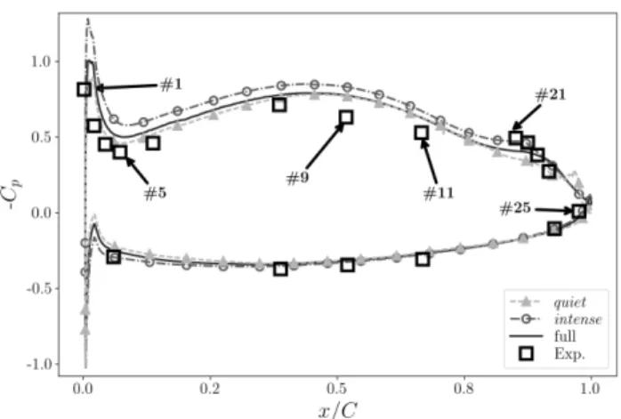
along the airfoil surface. The locations of the pin holes of 0.5 mm diameter in the center plane of the airfoil mock-up are identified with black squares in Fig.1 where the mean pressure was also recorded. The far-field acoustic pressure was measured using two 1/2 inch (12.7mm) PCB Integrated circuit piezoelectric microphones. The microphones were placed perpendicular to the jet flow direction on the suction and pressure sides of the airfoil at a distance of 1.36 m from the airfoil trailing edge. Both surface wall-pressure and far-field acoustic pressure were recorded at an acquisition frequency of25,600Hz with a NI-9234 module with 24 bits of resolution. The differential pressure is measured with a MKS Baratron 220D transducer.
Planar PIV measurements have been performed near the trailing edge region of the CD airfoil on the suction side and in the near wake region. The Planar PIV measurements were performed using a single5.5megapixel sCMOS camera. An Evergreen ND:YAG dual pulsed laser which yields up to
200 mJ of energy per pulse was used as the light source. The flow was seeded using a fog of glycerine droplets, of 1 µm typical diameter, injected upstream of the fan system driving the wind-tunnel. For the boundary-layer measurements of the suction-side a sampling frequency of 8 Hz was used. A magnification of0.73and a time delay of
6.3µsbetween pulses has been used, yielding a maximum
particle displacement of 14 pixels outside of the boundary-layer. A spatial resolution of about 0.21 mm was achieved by employing a multigrid iterative window deformation scheme wherein a four-step multigrid technique is applied starting from 96×96pixels to all the way down to24×24pixels with 75 % overlap27. A total of 4,000 images in double
frame mode were recorded. For the wake measurements a sampling frequency of 15 Hz was used. A magnification of 0.24 and a time delay of 24µs between pulses has been used, yielding a maximum particle displacement of 15 pixels outside of the wake deficit. A spatial resolution of 0.43 mm was achieved with this magnification and using the same multigrid technique up to a 16×16 pixels minimal correlation window with a 75% overlap. A total of 2,500 images in double frame mode were recorded. The sequences of images have been processed using Lavision’s commercial software DAVIS 8. In both sets of data, an initial average over 700 time frames is used to give the solver a better prediction for location of the correlation peak. Furthermore an elliptic weighting in the main shear direction is used to improve the maximum value of the correlation coefficient.
Numerical set-up
Figure 1. Detailed view of the refinement zones in the DNS
part of the domain. The labels specify the size of the cubic cells inside each refinement zone. Square symbols identify RMP locations for both experiments and simulation.
Similarly to the turbulent flow-regime case performed by Sanjoseet al.9, the direct numerical simulation is performed using the Lattice Boltzmann Method rather than the classical Navier-Stokes equations to proceed faster in time28,29 and
to account for actual experimental set-up more easily. This is even more crucial here as the observed unsteadiness of the acoustic and flow field requires a larger number of flow-through times t?=t U∞/C than for stable cases.
Installation effects from the wind tunnel are also known to play a significant role on the airfoil loading6.
The Lattice Boltzmann Method (LBM) solves the “mesoscopic” kinetic equations, i.e. the Boltzmann equation for a set of particle density functions with a collision source term, to predict macroscopic fluid dynamics. The collision source term is here represented by the simplest relaxation form known as the Bhatnagar-Gross-Krook (BGK) form30.
In the low Knudsen limit, frequency and wave-number are small relative to the lattice increments, and for the suitable choice of the set of discrete velocity vectors, the transient compressible Navier-Stokes equations are recovered through the classical Chapman-Enskog expansion, in the limit of low Mach numbers, i.e. M <0.3.31 The
molecular relaxation time τ of the BGK model is related to the fluid kinematic viscosity32. Thus to achieve the
physical laminar viscosity in the computational domain, what would be called direct numerical simulation (DNS),
sufficient mesh resolution is required for the given Reynolds number. The present simulation has been obtained with the commercial code PowerFLOW 5.1 from EXA Corporation in DNS mode. In that implementation, the discrete Lattice-Boltzmann equations are solved for 19 discrete velocities on cubic cells (D3Q19 method). For each discrete velocity, the particle equation is solved using a time explicit and spatially compact numerical integration based on the method of characteristics33,34.
To prevent using a hybrid method as in previous incompressible Large Eddy Simulation (LES) studies7,8,10,
the computational domain involves a thin slice of the corresponding full anechoic wind tunnel as described by Sanjoseet al.9,35. The spanwise domain extension has been
limited to 12% of the chord length because of the restriction of the current LBM to cubic voxels: it is however the same as for the 8◦ reference case, which was shown to be enough to capture the wall-pressure spanwise coherence length for the trailing-edge turbulent boundary layer at the present Reynolds number8,35. Thus, the same grid topology around the CD profile with zones of Volume Refinement (VR) of similar size that insured dimensionless distance to the wall y+ below 1. From one VR to another the grid
size is increased by a factor 2 by means of a conservative flux exchange36. To achieve the DNS requirements in the
first three VR around the profile the Mach number of the simulation is 4 times greater than the experimental one. All physical quantities obtained by summation of the momentum of the particle density functions are then rescaled afterwards using a dynamic pressure factor appropriate for this low Mach number flow. The actual voxel sizes of the first three VR is provided in Fig.1.
Figure 2. Sketch of the numerical setup showing boundary
conditions and sponge layers in shaded area and refinement zones with rectangular boxes.
Overall the three-dimensional grid has about 640 millions voxels with ten levels of consecutive grid refinements as shown in Fig.2. In the spanwise direction there are 1024 cells and periodic boundary conditions are applied. To mimic the anechoic environment, absorbing VRs (shown in gray
in Fig. 2) are set around the simulation box in which the laminar viscosity is gradually increased to mitigate the acoustic waves and prevent their reflection back into the computational domain. At the inlet, an axial velocity profile is prescribed which was measured at the exit of the wind-tunnel4 without airfoil, and slip walls are used to
prevent losses along the duct before the exit. No turbulent injection are considered to avoid any spurious noise. This is also representative of the little influence of residual inlet turbulence (below 0.4%) observed in various wind-tunnels on the separation bubble size on the CD airfoil37. The initial
condition for the simulation was taken from a preliminary simulation on a coarser grid with the first two finer VRs removed. The fully resolved simulation has been run for a total of 50 flow-through times, the first 10 flow-through times being a transient period to establish the flow field in the computational domain.
Aerodynamic results
In this section, we investigate the temporal and mean aerodynamic results from the DNS simulation in order to determine the characteristics of the boundary layer instability developing along the suction side of the airfoil. In particular, a wavelet analysis is used to identify meaningful events in the full time trace of the simulation. Based on this identification, the boundary layer state, which is closely related to the instability mechanism, and the wake development are compared for the unconditioned mean and the identified events with the available experimental measurements.
Overall flow topology
Figure 3 shows the instantaneous pressure and streamwise velocity fields at t∗= 26. The turbulence develops in the very aft of the airfoil suction side yielding the observed turbulent wake. The jet deflection by the cambered airfoil can also be noticed by the tilting of the jet shear layers that follow the direction of the turbulent wake shed by the airfoil. The jet shear layers are initially laminar and transition to turbulence through a vortex pairing that occurs downstream of the airfoil trailing-edge (shown by the white arrows) and therefore does not influence the airfoil loading. Including the jet effect in the simulation yields the proper airfoil loading and the direct noise emission in the near-field around the airfoil2.
Four characteristic time traces of the wall-pressure fluctuations at different locations on the airfoil suction side are shown in Fig. 4. The hashed zone corresponds to the transient regime of 10 flow-through times, where the abrupt fluctuations are related to the setting up of the airfoil loading on the resolved grid. Noticeably, the laminar recirculation bubble that was at the airfoil leading edge in the 8◦ reference case shifts toward the trailing edge, a flow bifurcation that was previously observed in the LES by Christophe et al. at a slightly higher incidence (6◦)10.
Later, in all time traces, large damped smooth oscillations are observed. They are related to the modulation of the pressure inside the potential core of the jet induced by the large coherent structures produced by the jet shear layer development observed previously. At RMP#5, a smooth laminar pressure signal is found. While the time trace of RMP#11 is very similar to the time trace of RMP#5,
Figure 4. Time trace of DNS wall-pressure fluctuations at different RMPs. vortex pairing vortex pairing vortex pairing vortex pairing
Figure 3. DNS instantaneous result in the full wind-tunnel
setup: (top) axial velocity contours; (bottom) pressure contours.
some high frequency oscillations of low amplitudes are superimposed to the smooth oscillations. Their amplitudes are intermittent which are the signs of turbulent spots and transition to turbulence. These bursts are more and more amplified toward the trailing edge as evidence in RMP#21 for which successive periods of calm and intense fluctuations can be clearly identified. Periods of intense fluctuations aroundt∗= 24,30and43are followed by longer periods of lower amplitude oscillations. The signal at RMP#25 shows the higher frequency content, and the amplitudes are more regular, although some modulation is still noticeable. The time-traces of the wall-pressure fluctuations demonstrate an intrinsic unsteadiness captured by the simulation. It is caused
by the instability of the turbulent transition in the aft part of the suction side as can be clearly identified by looking at snapshots of the flow field taken arbitrarily att∗= 12and t∗= 22in Fig.4. The flow features are visualized in Fig.5 using iso-surfaces of the second invariant of the velocity gradient, theQfactor. Note that despite the same level value of Qfor the iso-surfaces, the visualized coherent structures are quite different. For both snapshots, the boundary layer is laminar and no vortical structures can be seen up to two-thirds of the chord. Then close to RMP#11 location, natural instabilities grow in the laminar boundary layer as Tollmien-Schlichting waves (small ripples on the airfoil surface) that die out before the location where the flow separates (before RMP#21 location). The separated shear layer then becomes unstable, and this Kelvin-Helmholtz (K-H) instability yields rollers. This initial two-dimensional shear-layer roll-up is then followed by a significant three-dimensional distortion and break-up of the coherent vortices. Such a process has been described in details for several laminar recirculation bubbles by Marxen & Henningson38 and Joneset al.17 for
instance. In the present case, the strength and size of the
#25
#21 #11
#25
#21
#11
Figure 5. Q-criterion iso-surface coloured by the spanwise
velocity component taken att∗= 12(top) andt∗= 22(bottom). The spanwise location of the RMP#11, #21 and #25 are indicated with arrows.
is thin and long, yielding smaller vortices when it breaks up. Att∗= 22, for which intense fluctuations are present in
the time-trace of RMP#21, the roller is thicker and shorter, yielding larger and more intense vortices in the transition process. Larger coherent structures are consequently shed in the wake flow and stronger spanwise velocity can be noticed. Such large coherent structures shed in the boundary layer and in the wake flow were also observed in the Particle Image Velocimetry (PIV) instantaneous snapshots.
Wavelet analysis
The wavelet analysis is a well adapted tool for the study of such an unsteady evolution in order to link the unsteady pressure packets measured on the wall to the coherent structures formed in the turbulent regions39–42. In the present
analysis, a continuous wavelet transform is performed on discrete time series that demonstrate strong unsteadiness in Fig.4. The second derivative of a Gaussian (DOG) is used as wavelet function with a discrete Fourier transform to compute its convolution product with the windowed time signal for a set of scales efficiently. The time-signal for the second half of the simulation t∗>25 contains 15000 samples acquired with a sampling frequency of 71,392 Hz and is zero padded to the closest power of 2. The scales are distributed as fractional power of two with the smallest scale selected as twice the time-step and the maximum scale being the time duration of the signal42. The continuous wavelet
power spectrum for the time signal recorded at RMP#21 is shown in Fig. 6, below the time-trace of the pressure at the same location for which two main periods of strong fluctuations can be identified centered att∗= 31andt∗= 44. The cone of influence limiting the validity of the power spectrum due to the windowing of the signal by the wavelet base function is shown with the grey hashed area. Only the upper part of the spectrogram (or scalogram) with respect to that limit should be considered. To detect events, the Local Intermittency Measure (LIM)40,41 is defined as the ratio of the wavelet power spectrum over the time averaged wavelet power spectrum. The black plain contours highlight the area of powerful events defined by a LIM value greater than one. Events are detected for two main scales.
The two main bursts in the time-trace are well detected for a scale corresponding to 908 Hz which contains the maximum energy of the events. For the same scale, several other events are detected but with much shorter duration. Other events are detected for a scale of lower frequency between 50 Hz and 100 Hz. They correspond to local extrema of the smooth fluctuations induced by the jet development, which are more visible in the time-trace of RMP#5. The events detected for these two scales are strongly synchronized, suggesting that the jet flapping might influence the intensity of the pressure fluctuations. The main two bursts at t∗= 31 and t∗= 44 occurs after a major decrease of pressure by 20 Pa. In the spectrogram, the events detected for t∗ between 32 and 42 are not synchronized with the lower scale events detected within the same time period. During the two main bursts the wavelet power amplitude increases at scale corresponding to higher frequencies around 10 kHz highlighting a transfer of energy to the lower scales.
Figure 6. Wavelet power spectrum for RMP#21.
Considering the frequency resolution, only the events centered at 908 Hz are considered in the following analysis. Using the LIM signal for the scale corresponding to that frequency, events (grey diamonds) can be detected as shown in Fig7. They are sorted into local maxima (grey triangles pointing up) and minima (grey triangles pointing down) of the full pressure signal. From the flow visualizations available during the simulation length two distinct windows of one flow-through time are identified with the grey and dark-grey boxes in Fig. 7 corresponding to an intense and aquietflow-through time respectively. Some statistical analysis will be performed on both windows.
Figure 7. Events detection for RMP#21 at scale corresponding
to frequency 908 Hz. The detected events with the LIM maxima ♦are sorted out as local maximaMand minimaOof the pressure signal.
Boundary-layer analysis
As highlighted by the flow visualizations in Fig. 5 the boundary layer transition that occurs in the aft part of the airfoil suction side is drastically different in terms of the strength and the size of the Kelvin-Helmholtz rollers between the two different time instants. The events detected
with the wavelet analysis can be related to intense coherent structures passing at the probe location41. From the averaged field corresponding from theintenseandquietflow-through times identified in Fig.7and from the unconditioned average over the full time length of the simulation, the profile normal to the wall of the streamwise velocity is compared with the experimental averaged field obtained from the planar PIV measurements in the trailing-edge region in Fig.8. In thequietwindow, the flow has re-attached after the thinner separation bubble (pointed out att∗= 12in Fig.5), while in theintensethe above-mentioned recirculation bubble clearly extends up to the positionx/C= 0.92. The latter profiles are in better agreement with the experimental profiles in terms of shape and reversed flow amplitude, even though the larger experimental boundary-layer thickness suggests a thicker experimental recirculation bubble near the airfoil trailing edge. Therefore the unconditioned average boundary-layer profiles at the trailing-edge takes characteristic from the intenseevent, with a slightly thinner recirculation bubble.
Figure 8. Boundary layer extracted in the aft of the suction side.
The flow development along the suction side can be quantitatively assessed using the various boundary-layer parameters computed from the intense and quiet flow-through times, the unconditioned average over the full signal length and the experimental database from the PIV measurements in the trailing-edge region as well as the pressure coefficients measured at the pinhole locations shown in Fig. 1. Figure 9 shows the mean wall-pressure coefficient Cp=p−p∞/(0.5ρ∞u2∞). The
reference parameters (p∞, u∞ andρ∞) for the scaling of
Cpare measured at the nozzle exit for the two distinct event time windows and for the full time signal average to account for slight variations that could be induced by the jet shear layers, and measured with a Prandtl tube at the nozzle exit in the experiments. Significant variations are observed between the two conditional averaged fields. The most intense one compares well with the mean pressure measurements at the trailing edge, while the quiet one compares better at the leading edge. It should be mentioned that small pressure fluctuations appear on the suction side after the RMP#21 location for thequiet window. The unconditioned average Cp coefficient takes characteristic from both thequiet and intenseevent in the upstream part of airfoil and in the rear part of the airfoil respectively.
Figure 9. Mean pressure coefficient. Some labels of suction
side RMP probes are identified with numbers.
Figure 10. Boundary layer parameters: Mean friction (top) and
boundary layer shape (bottom) coefficients.
The mean friction coefficient on the airfoil Cf = τw/(0.5ρ∞u2∞) scaled with the nozzle exit reference
parameters, and the mean shape factor H of the boundary-layer are shown in Fig.10. The friction coefficient confirms the flow separation in the 25% aft portion of the airfoil for the intense time window, while it remains positive although close to zero, for the quiet time window. As a consequence of a thicker recirculation bubble in the experiments observed in Fig. 8, the friction coefficient shows larger negative values atx/C= 0.85than theintense window, but its global trend follows the same sudden growth towards the trailing-edge. The unconditioned average Cf coefficient takes characteristic from the intense event showing a slightly smaller recirculation zone. The boundary layer is in a completely different state in the two analyzed flow-through time windows. This is further confirmed by looking at the shape factorH =δ∗/Θ, which is the ratio of the displacement and momentum thickness of the boundary layer along the airfoil. In the simulation, below 70% of the chord the shape factor H along the suction side is around 2.4 (middle dashed line in Fig. 10), typical of a laminar boundary layer and similar for the two time windows and the unconditioned mean. It drastically increases to a maximum where the mean Cf is minimum for theintense time window. Flow separation occurs when H'3.5 (top dashed line in Fig.10). Close to the trailing edge the shape factor goes below 2.4 typical of the limit of turbulent flow separation and finally settles around 1.8 (bottom dashed line
in Fig.10), typical of an attached turbulent boundary layer. The shape factor H for the full signal average shows a similar trend than the intense time window, with slightly delayed increase and a lower maximum, still above the critical 3.5 value. For thequiettime window the H factor slowly increases from 2.4 (laminar boundary layer) to a maximum of 3 at 75% of chord at the location where the meanCfis minimal but slightly positive as a consequence of intermittent thinner recirculation as seen in the instantaneous fields (for example at t∗= 12in Fig.5). It then gradually decreases to the similar 1.8 value at trailing edge. The latter typical value for an attached turbulent boundary layer, is reached slightly earlier than for theintensewindow. Despite the small fluctuations seen in theCp levels, the boundary layer for that time window remains mostly laminar and attached up to the trailing edge where transition occurs. In the experiments the boundary layer shape factor behaves similarly as the numerical one in theintensetime window. In the recirculation bubble where the first measurements are available, the H factor is larger than in the intense conditional average due to the thicker recirculation bubble. It then similarly decreases to 1.8 at the airfoil trailing edge.
Wake profiles
To further characterize the consequence of the boundary layer state along the aft part of the airfoil on the downstream flow, the wake evolution is compared in Fig. 11 with planar PIV in the near-wake region at several locations downstream of the trailing edge. The wake statistics are again obtained for both time windows shown in Fig.7 and for the unconditioned mean over the full time signal of the simulation. As highlighted by the boundary-layer analysis, the two time windows represent two completely distinct behaviours. Thequiet flow-through time window presents a quasi-laminar attached boundary layer that transitions to turbulence with a thin and shorter recirculation bubble, and yields thin wake deficits in Fig. 11, while the detached boundary layer from theintenseflow-through time window yields a larger wake deficit and stronger turbulent levels. The full time average wake evolution is strongly influenced by the intense event. Although its wake width is smaller, its wake deficit and intensity are very similar to those from the intense window. The profiles extracted from the mean field of the intense flow-through time window agree well with the PIV measurements showing that it can be seen as a representative event of the experimental configuration. Still theintenseflow-through time window predicts a thinner wake deficit than the measurements, which is consistent with the previous boundary layer profiles.
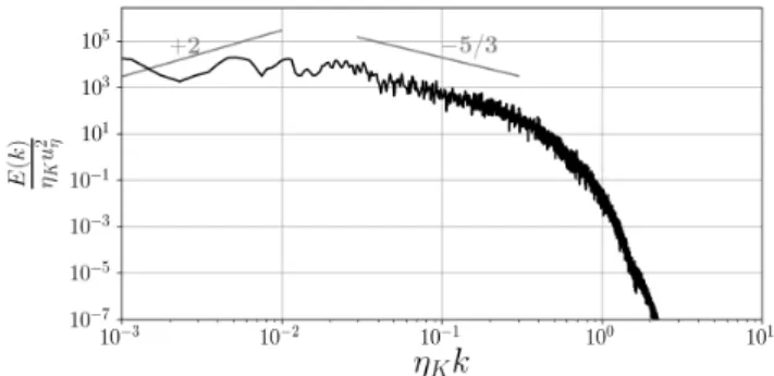
From the airfoil trailing-edge, the turbulent wake allows to assess the quality of the simulation by comparing the resolved turbulent scales with the Kolmogorov scales. For instance, the energy spectrum scaled by the Kolmogorov scale ηK and the velocity scale uη, computed from the laminar viscosity and the turbulent dissipation, is shown for a typical probe located inside the turbulent wake in Figure12. The spectrum shape shows in particular the scale separation with quite large inertial subrange with the typical −5/3
slope and a significant energy content up to the Kolmogorov scale. For large scales, modulation from the boundary layer instability appears as humps which participate in the energy
Figure 11. Streamwise mean velocity component (top) and
turbulence intensity in the wake (bottom).
production as they reasonably align with the typical +2
slope. Similar results are found in the suction-side turbulent boundary layer near the trailing edge. In can then be concluded that the current mesh density (Figure 2) allows resolving the turbulent kinetic energy spectra up to the Kolmogorov scale in the whole turbulent region: the last 15% chord length from the trailing edge and the wake.
Figure 12. Turbulent energy spectra normalized by the
Kolmogorov scales atx/C= 0.132andy/C= 0.007.
To summarize these first aerodynamic results, theintense events are therefore seen to be more representative of the flow captured by the experiments in terms of mean loading (Cp distribution), mean boundary layer shape near the trailing edge and wake development. They are the dominant features yielding the mean flow and the main flow statistics as observed on the characteristics from full time signal average .
Noise results
In this section, we investigate the noise sources and the noise radiation from the DNS simulation, emphasizing the emission of tones. Based on the events identified from the
wavelet analysis, the wall-pressure fluctuations developing along the suction side in the boundary layer and emitted acoustic sound spectra from the quiet, intense events and the full time signal is compared with available experimental measurements.
Noise sources: wall-pressure fluctuations
The next step is to analyse the impact of these different time frames on the wall-pressure fluctuations born in the boundary layer that provide the trailing-edge noise sources. From the temporal evolution shown in Fig.4, the power spectral density of the wall-pressure fluctuations are computed for the two short time windows calledintense andquietidentified in Fig. 7, and for the full signal length recorded for t∗>
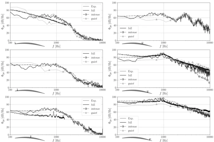
26. These spectra are obtained using a Welch periodogram technique with 50% of overlap, yielding 3 time blocks for the intenseandquietsignals and 8 time blocks for the full length signal. When available the experimental measurements are compared with the numerical results in Fig.13. Experimental measurements in the laminar or very quiet part of the airfoil is quite challenging. Some spectra were contaminated with electric noise for levels below 40 dB/Hz. Hence when occurring, the spectrum part with high standard deviation has been removed from the comparison. This was the case for RMPs #3, #5, #6, #7 and #9.
Fig. 13 clearly shows that the full length signal from the simulation takes its characteristics from both the typicalintenseandquietframes, which make the particular distinction provided by the wavelet analysis very relevant. At RMP #1 close to the leading-edge, the experimental spectrum has low levels typical of a laminar boundary layer. Its shape is a characteristic broadband turbulence impingement spectrum caused by the residual low turbulent level in the wind tunnel with large integral scales43. This is globally captured by the three processed signals from the simulation. At RMP #5, for all three numerical datasets, the amplitude levels below 300 Hz drop and the rest of the spectrum remains the same.
At RMP #9, small tone amplitudes are emerging at frequencies 700, 850 and 1000 Hz. The quiet and intensetime window spectra differ essentially in the range [400,1500] Hz, where a large hump is captured only in the intense spectra. The same hump will be found in all the other probe spectra for theintense time window. Globally for the first half of the chord the signal processed from thequiet time window agrees better with the experimental spectra up to 2 kHz which confirms the observations made on airfoil loading shown in Fig. 9. At RMP #11 humps at high frequencies (one is centered at 3000 Hz and the other two are its harmonics) are obtained with both time windows. These humps are frequency traces of the small pressure fluctuations that initiate the transition to turbulence. This again highlights that these local perturbations are not modified by the downstream boundary layer state. They do not appear to have a different signature for the two time windows analyzed. These fluctuations are not the consequence of a feedback mechanism rather an inherent instability of the boundary layer at this location.
The critical change in the pressure fluctuations from RMP #21 to RMP #25 shown in Fig.13should be related to the H factor of the boundary-layer. For the intense window,
the high frequency content in the spectra (f >5000 Hz) increases drastically between RMP#21 and #25. In between these locations (0.85< x/C <0.95) the boundary layer is largely detached and tends to reattach (dropping levels ofH in Fig.10) just before the trailing edge. For thequietwindow, the high-frequency levels in the spectra (f >5000Hz) are 20 dB higher than for theintensewindow. It also influences the spectra computed over the full signal length and agrees with the experimental levels. This part of the spectra is related to the inner part of the boundary-layer and representative of a more attached boundary layer with smaller turbulent scales. The broadband hump in the range [400,1500] Hz that appears in the intense time window and in the spectrum computed from the full time signal is in good agreement with the experimental spectrum. The clear tones that appear at850Hz and 1000 Hz in the experimental measurements do not appear in the numerical results. On the one hand theintense andquiettime windows are too short to provide a sufficient frequency resolution. On the other hand, the spectrum obtained from the full time length show multiple thicker tones at frequency 550, 670, 840 and 1000Hz. Measured tones are reported for both experimental and numerical results in Tab.1. Because of the low frequency resolution in the numerical results, the center peak value reported in Tab.1 has been obtained by finding the local maxima from the spectra in linear scale (not shown here). The good agreement of the numerical and experimental spectra for the last probe locations highlights the ability of the present simulation to capture the peculiar laminar boundary layer transition to turbulence at the end of the suction side. Overall the maximum levels of the wall-pressure fluctuations along the airfoil suction side are a broadband hump around 1000 Hz and are therefore dominated by the intense time windows. The quiet ones only contribute significantly to the high frequency range (smaller vortical scales).
To summarize the wall-pressure spectral content along the suction side, the amplitudes for three characteristic frequencies that appear in Fig.13are shown on the profile surface in Fig.14. The colour maps are clearly dominated by the characteristics identified in theintensetime window with the boundary layer analysis. The strongest amplitudes are concentrated in the rear part of the airfoil where the transition occurs. For the lowest frequency, the higher amplitudes show the reattachment point at about 95% of the chord. Quite constant high amplitude levels are seen in the last 80% of the chord for the frequency centered on the broadband hump in the wall-pressure spectra. For both 560 Hz and 1060 Hz, large levels can be observed on the whole surface of the suction side. The higher frequency shown in Fig. 14 has a very distinct distribution. Significant levels are only visible in two areas in the last 80% of the surface, and at the begin of the transition at 65-70% of chord as identified in Fig.10. In between a silent zone identifies the beginning of the recirculation bubble which halts the natural transition process.
Far-field acoustic pressure
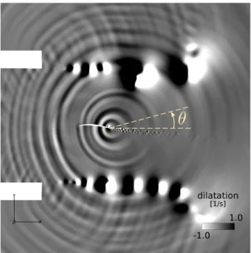
The radiated acoustic field is first shown in Fig. 15by the iso-contours of the dilatation field 1ρ∂ρ∂t which is computed here between two snapshots delayed by 70 ms. The overall field in the full computational domain clearly shows the
Figure 13. Wall-pressure fluctuations at several locations on the airfoil suction side. Left: first half chord sensors RMP#1, #5 and #9 from top to bottom. Right: second half of the chord sensors RMP #11, #21 and #25 from top to bottom.
Far-field (exp.) FWH wall p (exp.) wall p (DNS) Wavelet DMD SPOD LST
579 544 550 370 391
737 670 670 630 660 703
864 781-860 860 840 908 760
991 990 1000 1080 1010 1000
1100 1200, 1300 1460 1300 1332
Table 1. Tones found in all experimental, numerical and theoretical analyses.
reattachment point recirculation bubble inception of transition
Figure 14. Wall pressure amplitudes for three frequencies: 560
Hz, 1060 Hz and 3000 Hz.
dipole-nature of the radiated noise, and stresses that the main noise mechanism is the diffraction at the trailing edge. The latter has a wavelength corresponding to a frequency of about 1 kHz, which corresponds to the frequency range
where the highest wall-pressure fluctuations are obtained from theintensebursts. The discontinuity in the levels of the fringes emitted from the airfoil trailing edge also stresses the intermittency of the radiated sound.
The diffraction from the nozzle lips is also clearly seen, which will affect the noise directivity (distorted lobes) compared with a free-field dipole. Some reflection can be observed at the edge of the nozzle lips. The diffraction by the jet shear layer is also found to be negligible as expected at this low Mach number.
The corresponding DNS spectra in the far-field shown in Fig.16are computed from the wall-pressure fluctuations on the airfoil for the full signal length recorded for t∗>26
with the Ffowcs Williams and Hawkings analogy44 using
an advanced time formulation45 as implemented in the
in-house SherFWH code. Since the airfoil is not moving this is equivalent to Curle’s analogy. The spectrum is computed using a Welch periodogram technique with 8 time blocks for the full length signal and using a 50% of overlap between consecutive blocks. A frequency resolution of 20 Hz is obtained. To account for the full span of the
Figure 15. Acoustic waves shown by an instantaneous field of the dilatation field in a plane at mid-span of the airfoil.
experimental setup, the obtained spectrum is scaled by a factor (Lexp/Lsim)2 assuming uncorrelated noise sources
along the airfoil span. Good spectral shape and sound levels are obtained compared with measurements. Higher tones are however found below 800 Hz and broadband humps extend to 2000 Hz.
Figure 16. Acoustic spectra at 1.36 m from the airfoil trailing at
90◦degrees from the jet streamwise velocity.
The main tones visible in the acoustic spectra in linear scale (not shown) are reported in Tab.1.
Visualizations of the event signature
In the previous sections, the intermittency of the flow and the radiated noise has been evidenced and most aerodynamic and noise features have been shown to be dominated by certain time-windows in which intense vortex bursts are seen. We now try to connect the observed noise radiation to theintense events stressed by the wavelet analysis.
In the identified intense time windows in Fig. 7, a total of 18 events are detected with 9 local maxima and minima of pressure fluctuations respectively. From instantaneous frames recorded at frequencyfs= 14,500 Hz in the mid-span of the computational domain, conditional averaging is
performed separately on both event types. The mean static pressure over the intense flow-through time is subtracted from the pressure obtained by the conditional averaging. The signatures of the two event types are identical but with opposite pressure levels46. In Fig.17, pressure fluctuation
contours of the signature from the local maximum events are shown. The same conditional averaging is performed for shifted snapshots around the detected events providing a time animation of the event signature (provided as additional material). At the end of the suction side of the airfoil, successive lobes of pressure are propagating towards the trailing-edge. The signature centered on the events shown in Fig. 17 is synchronized when the last lobe has passed the trailing-edge and has been divided into two distinct lobes (in red downstream of RMP#25). While these pressure lobes in the boundary layer convect downstream, acoustic pressure waves are emitted and propagate upstream. Their levels are about 10 times smaller than the pressure waves convected along the suction side. The signature centered on the events shown in Fig. 17 is also synchronized when one acoustic lobe is centered around RMP#11 where small pressure fluctuations can be noticed in the iso-contours. From the time-animation, no modifications of these small pressure fluctuations at RMP#11 can be seen with the passing of the acoustic wave front. These synchronous visualizations allow clear identification of the aeroacoustic mechanism previously discussed by many authors14,17. In the present
case, the acoustic waves are emitted from the trailing-edge and caused by the diffraction of the coherent structures from the boundary layer. The wave fronts obtained are identical to the dilatation fronts shown in Fig. 15. Here they can be clearly related to the diffraction of the large coherent structures from the boundary layer instability at the trailing edge of the airfoil. No influence of the upstream propagating waves on the hydrodynamic structures could be identified.
11 21 29 25 Pressure Fluctuations [Pa]
Figure 17. Pressure fluctuations from the local maximum
events obtained in RMP#21 during theintenseflow-through time window.
Modal and stability analysis
From the analysis of the noise sources, the noise radiation including a broadband hump and the emission of tones have been related previously to the detached boundary layer in the rear part of the suction side that occurs during intense events. Two modal analysis are performed to investigate the
dominant modes in the boundary layer and in the near wake that drive this particular acoustic signature. Finally a linear stability analysis is performed to investigate the growth of waves in the boundary layer and to link the tone emissions to the instability location of the Kelvin-Helmholtz waves.
DMD analysis
The dynamic mode decomposition (DMD) is a recent modal analysis23 that allows identifying the dominant motions involved in a flow field regularly sampled in time. Its principle is to map a time sequence with a linear operator that describes the evolution of one snapshot to the next. Given n+ 1snapshots of the flow field, the time sequence of then last instantsV2n+1 can be approximated from the sequence of thenfirst instantsVn
1 by means of the DMD:
V2n+1=V1nS (1)
where S is a n by n matrix, that can be obtained by the Singular Value Decomposition (SVD) ofVn
1. The complex
eigenvalues(µr, µi)of the matrix S provide a description of the dynamics of the flow-field which can be related to a frequency. From the eigen problem resolution, they can be associated to an amplitude A which describes the predominance of the given modes in the dynamics of the flow-field.
From the volume data recorded during the intense time window, a spanwise average is computed for the 230 snapshots sampled at 14,500 Hz. Only the pressure and velocity components are considered to describe the flow dynamics. The DMD provided as a module of the YALES2 CFD flow solver47 has been used. The time averaged flow field of the sequence is removed, consequently the eigenvalues lie on the unit circle as shown in Fig. 18, i.e., each mode has zero growth rate and oscillates at a real frequency. Their distribution is symmetric along the imaginary axis as the initial snapshots are real values. The strongest modes with darker filled circles have small imaginary part and a real part close to one.
Figure 18. Eigenvalues of theSmatrix of DMD decomposition.
Each eigenvalue is marker is colored and scaled by the amplitude of the mode. The unit circle is shown in dot-dashed line.
The amplitudes associated with each mode is provided as a function of frequency in Fig. 19. The amplitude decays rapidly after 2000 Hz. The dominant modes have frequencies 630 Hz, 60 Hz, 370 Hz, 760 Hz, 1010 Hz and 1460 Hz in ranking order. These frequencies are reported in Tab. 1. The dominant DMD mode is shown in Fig.20. The pressure
Figure 19. Amplitude distribution of the DMD modes as
function of frequency.
field of the mode highlights the Kelvin-Helmholtz instability in the aft part of the suction side which was captured by the event signature of the wavelet analysis in Fig. 17. The velocity fields of the mode show the same lobes but distorted by the shear in the boundary layer. Significant lobes persist in the wake for the velocity components while they vanish for the pressure field. For pressure and velocity the first lobes appear at the location of the RMP #21 which was used for the event detection in the wavelet analysis.
Figure 20. Dominant DMD mode at frequency 630 Hz. Modal
shape for the pressure field (top), streamwise velocity (bottom left) and vertical velocity (bottom right).
The second main DMD mode at 60 Hz is shown in Fig.21. This low frequency mode is a remaining of the removed averaged field of the short duration of the time sequence. It mainly stresses the breathing of the laminar recirculation bubble and the pressure fluctuations in the potential core of the jet.
SPOD analysis
Dynamic mode decomposition is well-suited for identifying high-amplitude tones, but is not ideal for investigating broadband turbulent flow dynamics25. In this section, we use spectral proper orthogonal decomposition (SPOD) to study
Figure 21. Second DMD mode at frequency 60 Hz (same field order as Fig.20).
the broadband behavior of the turbulent flow associated with the recirculation bubble and the airfoil wake.
Spectral proper orthogonal decomposition, which is also sometimes called classical or frequency domain POD, was introduced by Lumley24 and is derived from a space-time
optimization problem for statistically stationary flows. This form of POD identifies energy-ranked modes that each oscillate at a single frequency and are orthogonal to other modes at the same frequency. Each mode evolves coherently in space and time and can thus be regarded as a coherent structure. Additionally, Towne et al.25 recently showed that SPOD is closely related to DMD. Specifically, SPOD modes are optimally averaged DMD modes obtained from an ensemble DMD problem that incorporates data from several realization of a turbulent flow. Accordingly, using SPOD to study the broadband behavior observed for the CD airfoil is a natural extension of the DMD analysis presented in the last section. SPOD was recently applied to an airfoil with a fully attached boundary layer by Abreuet al.48, while the present paper is the first to apply it to a separated airfoil to the best of our knowledge.
SPOD modes are obtained via an eigen-decomposition of the cross-spectral density tensor, which is estimated using Welch’s method with 80% overlap, leading to ten flow realizations within the intense flow window and a frequency resolution of 110 Hz. Since the airfoil is homogeneous in the spanwise direction, each spanwise Fourier component can also be considered independently49. We found the spanwise mean component to dominate, so we focus on this component in what follows (this also justifies our choice to use the spanwise mean for the previous DMD analysis). Computing SPOD modes also requires the choice of an appropriate inner product, for which we use the classical Chu compressible energy norm50. Since the numerical solver
considers a low compressible isothermal flow, only the pressure and velocity components are required.
The SPOD analysis provides an optimal orthogonal mode basis for the flow realizations at each frequency. The energy associated with the first three modes is shown in Fig. 22, as well as the total energy spectra computed from the ten modes. The first mode is about an order of magnitude more energetic than subsequent modes, and therefore accounts for most of the flow energy, for frequencies between 110 Hz and 2200 Hz. The first mode presents two main lobes centered
on 660 Hz and 1320 Hz. These frequencies are reported in Tab. 1. Considering the low frequency resolution inherent to the method for providing a convergent estimate of the spectral densities, they correspond to the frequencies of the DMD dominant and fifth modes respectively. The spectra of the SPOD modes decay at low frequencies contrary to the DMD amplitude spectra which find the second dominant mode for the minimum frequency. This highlights that the present analysis by means of the periodogram technique is better suited for strongly varying flow sequence as presently analyzed.
Figure 22. Eigenvalues of the SPOD analysis as a function of
frequency. The main local maxima are highlighted with arrows The pressure and velocity fields of the dominant mode are presented for the frequency of the first hump in Fig.23. The Kelvin-Helmholtz modal shape can be clearly identified on the pressure field between RMP #21 and #25. While the lobes for the pressure field vanish rapidly in the near wake, they are quite significant for the velocity component fields. This is even clearer for the frequency of the second hump shown in Fig. 24. For that frequency the lobe amplitudes of the velocity component are dominant in the near wake. For the streamwise velocity, the upper lobes shed from above the recirculation bubble as a consequence of the Kelvin-Helmholtz instability, while the lower lobes are grazing on the surface then merging with the vortex shedding shed by the blunt trailing-edge. The transverse velocity lobes cover both shedding areas, probably creating a coupling or a momentum transfer between these two instability mechanisms. The pressure field at 1320 Hz can also be related the wavelet event signature shown in Fig. 17, suggesting that the same noise mechanism is at work. In addition to the lobes on the airfoil surface, acoustic waves with opposite amplitudes are emitted from the trailing edge and propagating upstream. The coupling between the structures on the airfoil surface and in the near-wake suspected by their synchronism in the wavelet event is confirmed by this SPOD optimal basis, and this mechanism is related to the acoustic wave emissions.
Linear stability analysis
Some of the spectral properties of the flow seen above are now related to linear instabilities of the mean boundary layer profile. Two different mean flows are considered. The first is computed over thequietwindow and the second is computed over anintensewindow.
Figure 23. Dominant SPOD mode at frequency 660 Hz.
Figure 24. Dominant SPOD mode at frequency 1320 Hz.
The linearized Navier-Stokes equations are written in curvilinear ξ−η coordinates with the η coordinate consisting of straight lines perpendicular to the surface of the airfoil and ξ orthogonal to η. The value η= 0 traces the surface of the airfoil and ξ varies from 0 to 1 from the leading-edge to the trailing-edge along the suction side of the airfoil. Since the mean-flow is slowly-varying along the airfoil, i.e., in the ξ-direction, it is valid to perform a local stability analysis at each value ofξ. Accordingly, the fluctuations are assumed to take the form of two-dimensional traveling-waves of the form
q0(ξ, η, t) = ˆq(η)eiαξ−iωt. (2) The properties of the flow allow several additional simplifications. First, since the boundary layer on the airfoil is thin (even for theintensewindow), the classical boundary-layer approximation is valid and the second ξ-derivatives can be neglected. Second, the curvature of the airfoil is small within the region of interest, i.e, along the latter part of the suction side of the airfoil. Because of this, the grid can be considered to be locally Cartesian at eachξ-station along the airfoil with the transverse coordinate aligned with the localη-ray. This eliminates a large number of terms in the linearized equations. Third, since the Mach number is small, the spatial variation of thermodynamic quantities can be neglected and are thus set to their free-stream values. Finally, the η-velocity and the ξ-derivatives of the mean-flow are neglected for consistency with the locally-parallel approximation.
Inserting the form of the fluctuation given by Eq. (2) into the linearized equations, applying the preceding simplifications, and numerically discretizing the equations in theη-direction leads to an equation at eachξof the form
[−iωI+iαA+B]qˆ= 0. (3) For the present analysis, the equations are discretized using sixth-order central finite-differences with summation-by-parts closure51. Characteristic boundary conditions are
applied at the airfoil surface52 and radiation boundary
conditions are enforced at the far-field η-boundary using a super-grid damping layer53. Solutions satisfying Eq. (3) exist
only for certain combinations ofωandα, which define the local modes of the flow.
One potential source of the observed tones would be the presence of an intrinsic oscillation related to absolute instability of the re-circulation bubble during intense periods in the flow54. Previous investigations have shown that the separated region supports a Kelvin-Helmholtz instability that can in some cases become absolutely unstable. Within the weakly nonparallel analysis, absolute instabilities are described by modes that satisfy Eq. (3) as well as the zero-group-velocity condition55.
∂ω
∂α = 0. (4)
A mode ω0, α0satisfying these conditions is said to be absolutely unstable if ωi0>0. In this case, the mode will grow at its source leading to an intrinsic oscillation that is capable of producing a discrete tone at the frequency ω0r . The subscriptsrandiindicate the real and imaginary parts, respectively. Modes that satisfy Eqs. (3) and (4) correspond to saddle-points in the complex α-plane and cusps in the complexω-plane. In this work,ω0is computed by locating
cusps using a grid of complexα-values. The procedure has been validated by reproducing values ofω0for an analytical
wake profile reported by Huerreet al.55and Joneset al.17.
Figure 25. Maximum temporal growth-rate and absolute growth
rate from the absolute stability analysis. The absolute growth-rate ω0
i of the Kelvin-Helmholtz mode is shown in Fig.25as a function of chord-wise position along the suction side of the airfoil for the mean flow from anintensetime window. Since it is negative everywhere, the Kelvin-Helmholtz waves are not absolutely unstable. Also shown is the maximum value ofωitaken over all real-values of α. Since this value is positive (over the latter part of the airfoil) but ω0i is negative, the Kelvin-Helmholtz waves are
convectively unstable (CU) in this region. The re-circulation bubble is absolutely stable (S) but convectively unstable (CU), which can be explained by the low level of the reverse flow of -2 m/s (12% of the mean incoming velocity). On the other hand, the attached mean flow from thequiet window does not support unstable Kelvin-Helmholtz waves at all.
Figure 26. Maximum spatial growth-rate from the spatial
stability analysis.
The spatial growth of periodic disturbances is next studied by finding solutions of Eq. (3) for real values of ω. Only the intense window is considered since the quiet window does not support growing Kelvin-Helmholtz waves. The maximum value ofαiis plotted as a function ofξin Fig.26. The cumulative amplification of the Kelvin-Helmholtz waves as they convect down the airfoil can be measured by the amplification factorAgiven by:
A(ω) = exp − Z 1 ξ0 αi(ω, ξ)dξ . (5)
Here, ξ0 is the (frequency dependent) location where
the Kelvin-Helmholtz wave first becomes unstable. The amplification factor is plotted in Fig. 27. The broad peak centered at 900 Hz matches well with the broad hump observed in the near- and far-field PSD. This confirms that Kelvin-Helmholtz wave, rather than Tollmien-Schlichting waves, constitute the dominant instability mechanism leading an acoustic response in this flow, as is observed from the visualizations of the event signature obtained during the intensewindow in Fig.17.
Figure 27. Amplification factor from the spatial stability
analysis.
Using the model proposed by Kingan & Pearse56, the eigenvalues obtained from the spatial stability analysis
can also be used to obtain a crude estimate of the tonal frequencies. The hypothesis underpinning this model is that the tones are produced by a feedback loop between growing downstream-propagating instability waves and upstream-propagating acoustic waves. These waves reinforce each-other only if the total phase change over the loop, which is given by the expression
Φ (ω) =
Z 1
ξ0
αr(ω, ξ)dξ+π+ ω
1−M, (6) equals an integer multiple of 2π. This model predicts the appearance of tones at 391, 703, 1012, and 1332 Hz, as shown in Tab.1. While some of these values seem to match tones observed in the data and others do not, it is important to note that the model contains several uncertainties that could lead to discrepancies. More precise predictions of the tonal frequencies will be obtained in the future using a global stability approach.
Conclusions
The first compressible direct numerical simulation of the flow-field around a Controlled-Diffusion airfoil has been achieved at a low angle-of-attack (5◦) and a high Reynolds number based on the chord length (1.5×10⁵), in its
actual acoustic test set-up for which unstable tonal noise radiation had been previously reported. The installation effects induced by the wind-tunnel large anechoic room and finite-size nozzle have thus been included. Moreover unusual long run times have been collected (50 flow-through times) to be able to pinpoint the flow intermittency. Good overall agreement with experimental data is achieved for the wall-pressure, wake statistics, and far-field sound. Proper resolution up to the Kolmogorov scale is also demonstrated in the turbulent parts of the flow.
Time traces and flow visualizations have been the first qualitative evidences of the flow intermittency in the present configuration. A wavelet analysis has then quantified the unsteadiness of the boundary-layer development, and shown the presence of quiet and intense time windows for the first time. During a typical quietframe, the initial laminar boundary layer transitions to turbulence more progressively through a Kelvin-Helmholtz instability yielding long and thin rollers that break up into smaller vortices. The mean flow is fully re-attached close to the trailing edge, and a thin turbulent wake develops away from the airfoil. During a typicalintensewindow, the initial laminar boundary layer detaches after two-thirds of the chord, and the detached shear layer undergoes a Kelvin-Helmholtz instability and transitions to turbulence suddenly, producing large and compact rollers. The latter quickly break up into smaller vortices and the flow reattaches before the trailing edge, yielding a thicker turbulent wake.
Analysis of the wall-pressure fluctuations in the aft region of the airfoil, that can be seen as the trailing-edge noise sources, emphasizes the contributions of the events in both time windows. The events in the intense time windows significantly contribute, mostly around 1000 Hz, and show several tonal peaks. The signature of these events then allows the identification of the hydrodynamic mechanisms responsible for the emission of a strong dipolar acoustic field
in the same frequency range. The tonal noise is therefore not seen to come from Tollmien-Schlichting waves forming in the laminar boundary layer as previously conjectured, but rather from a Kelvin-Helmholtz instability that yields rollers of different shapes and strengths that break down at the trailing edge. Moreover installation effects are shown not only on the airfoil loading, the noise directivity as previously reported, but also on the possible transition mechanism on the airfoil and a possible coupling between the low-frequency jet flapping and the development of the intense bursts, possibly enhancing the observed tonal noise.
Both the Dynamic Mode Decomposition and the Spectral Proper Orthogonal Decomposition confirm the Kelvin-Helmholtz instability as the dominant flow phenomenon in the airfoil aft for this particular flow condition. The SPOD and wavelet event signature also suggest a coupling between the rollers induced by the Kelvin-Helmholtz instability on the airfoil suction side and the wake vortex shedding induced by the sudden transition to turbulence on the airfoil pressure side near the trailing edge, and the airfoil trailing-edge bluntness. Both analyses also clearly show acoustic waves emitted from the trailing-edge caused by the strong coherent structures breaking down at the trailing edge and possibly enhanced by this flow coupling between the suction and pressure sides.
Finally a linear stability analysis stresses that the Kelvin-Helmholtz waves are only convectively unstable (not absolutely unstable) and that the recirculation bubble is absolutely stable. This analysis may also suggest an acoustic feedback loop between the transitional zone and the airfoil trailing edge. Yet only a global stability analysis might be able to provide an definite answer.
Assessment of errors in measurements
Wind tunnel operation
The open wind-tunnel in Universit´e de Sherbrooke is controlled in temperature and fan power. The atmospheric pressure and humidity in the anechoic room are not controlled and no associated errors have been made. No noticeable variations in the measurements made on different days have been observed. The outlet velocity is measured with a Pitot tube in the nozzle wind tunnel. A water manometer is used to measure the reference velocity yielding to 0.1% relative error in the stagnation pressure. The mock-up is located in between rigid plates for which the slits holding the airfoil have been cut with a laser with an accuracy of±0.125 mm.
Airfoil loading measurements
The Baratron transducer has an absolute error of 0.15% of the reading-range yielding to a maximal absolute error of ±0.2 Pa. It yields a relative error of 0.1% based on the reference stagnation pressure. The latter has its own error provided above.
PIV measurements
One classical error quantification for PIV measurements and related post-processing is to consider an uncertainty in the displacement measured is of the order of 0.1 pixel57.
Considering a minimum displacement close to the wall of 3 pixels and a maximum displacement 14 pixels outside of the boundary layer or the wake, it would yields a relative error ranging between 3.3% to 0.7% of the mean velocity.
More advanced estimations58 would require the post-processing to be performed again or the measurements to be performed with different camera settings and seedings which was not possible in the present study.
In addition to the velocity measurement precision, the localization of the wall plays an important role in the boundary layer study. This localization fully rely in the physical calibration of the camera sensors and the error is in the order of half of the correlation window size. In the computation of the friction coefficientCf, this is the leading-error in the estimation of the velocity gradient normal to the wall. It also causes discontinuities of velocity gradients which is corrected by using a Gaussian filter function with a 6 point kernel size on the velocity profiles extracted normal to wall. The velocity gradient is then computed using the one-sided forward second order finite difference, which expression (4.5.5) can be found in Hirsch’s book59. The laminar viscosity is estimated from the Sutherland’s law based on the controlled temperature of the wind-tunnel and the density of dry air at this temperature. A rough estimate would be that theCf function is obtained with an accuracy of 50% relative error because of the wall localization. Taking a velocity variation of0.1U∞over one interrogation window
of0.21mm, the error made on theCf would be0.4×10−2.
Far-field acoustic measurements
Far field measurements were done using, PCB ICP microphone which have a variation of sensitivity of 41.2 % or±1.5 dB in the range of 100 to 20,000 Hz. The calibration of all microphones allows correcting the sensitivity at the frequency of the calibrator only, thus the error associated with the sensitivity remains. A Larson Davis 200 calibrator has been used which has an uncertainty of 4.7% or ±0.2 dB. In the computation of autospectra of acoustic pressure is measured for 30 s. The time signal is divided into blocks of 1 s with 75% of overlap yielding a numberNs= 120of total sets on which the autospectra is computed and averaged out. The estimation of error in the autospectra evaluation can be computed using the formula (19) derived by Bendat60:
=√1
Ns
(7) yielding 9.1% of relative error or±0.4 dB.
Wall pressure fluctuation measurements
The wall pressure remote microphone probes are equipped with a Knowles microphone (FG 23329 P07) which sensitivity varies by 100% or±3 dB in the range of 100 to 10,000 Hz. This sensitivity variation and the attenuation from the remote system are corrected over the whole frequency range by means of a calibration procedure for which a white noise signal is simultaneously measured by the probe and a reference microphone. The latter is a TMS microphone (130P10 ICP) with a sensitivity variation of 58.5% or ±2.0 dB in the range of 100 to 20,000 Hz. This 1/4 inch microphone was also calibrated using Larson Davis 200