- BarcelonaTech
Facultat d’Inform`atica de Barcelona (FIB)
Master in Innovation and Research in Informatics (MIRI)
High Performance Computing (HPC)
2016-2017
|
Spring Semester
Application Performance Evaluation
using Deep Learning
Author: Simon S¨oderlind
Advisor:
Daniel
Jimenez
Computer Architecture
Department (DAC)
Supervisor:
Judit
Gimenez
Barcelona Supercomputing
Center (BSC)
First of all, I would like to thank Jesus Labarta and Judit Gimenez for proposing and giving me the opportunity to work on this exciting project.
I would like to give another thank you to Judit Gimenez for her supervising role for this thesis.
Thank you Daniel Jimenez for agreeing and taking on a tu-toring role.
Finally, I would also like to thank all my family for their constant support.
Developing software for exascale systems will become even more challenging than for today’s systems. Methods for eval-uating the performance of applications and identifying po-tential weaknesses are essential for reaching optimal perfor-mance. Though the tools available today are not widely used, and generally require some expert knowledge.
In recent years different deep learning techniques have en-joyed great success in various fields, and especially in image recognition. Though it is still to find its way in to the area of application performance evaluation.
This work will take the first step towards introducing deep learning to the area of HPC performance evaluation, opening the door for others. Convolutional neural networks will be fed images of timeline views of HPC applications and will identify the intrinsic behavior of the application and return some principal performance metrics.
The results show that deep learning techniques indeed can be utilized for evaluating the performance of parallel applica-tions, with the main limitation for its success being the sizes of the data sets available. Furthermore a number of excit-ing directions for takexcit-ing the next step utilizexcit-ing deep learnexcit-ing techniques with performance evaluation are suggested.
Contents
1 Introduction, Motivation and Goals 1
1.1 High Performance Computing 2
1.2 Performance Evaluation 3
1.3 Deep Learning 5
1.4 Related Work 5
1.5 State of the Art CNN Architectures and Applications 6
1.6 Paper Outline 7
2 Performance Evaluation 9
2.1 POP Performance Metrics 9
2.2 BSC Tools Parallel Performance Analysis Suite 11
2.2.1 Extrae 11
2.2.2 Paraver 12
2.3 Analysis Process 14
3 Deep Learning 15
3.1 Neural Networks 15
3.1.1 Artificial Neural Networks 16
3.2 Training 21
3.2.1 Error Quantification 21
3.2.2 Backpropagation 22
3.2.3 Weight Initialization 25
3.3 Convolutional Neural Networks 26
3.3.1 The Convolution Layer 27
3.3.2 Pooling Layer 28
3.3.3 Example Architecture 29
4 Methods 31
4.1 Software 31
4.2 Hardware 32
4.3 Neural Network Models 32
4.3.1 VGG-19 33 4.3.2 Custom Models 34 4.4 Data Generation 35 4.4.1 Data Pre-Processing 36 4.5 Training Process 37 5 Experiments 39 5.1 Unprocessed Data 39 5.2 VGG-19 Models 40 5.2.1 Classification 40 5.2.2 Regression 41 5.3 Custom Models 42
5.4 Importance of Large Data Sets 43
6 Discussion, Conclusions and Future Work 45
6.1 Discussion 45 6.2 Conclusions 46 6.3 Future Work 46 References 47 Appendices 56 A Detailed Results 57
A.1 Unprocessed Data 57
A.2 VGG-19 Classification Models 58
A.3 VGG-19 Regression Models 59
A.4 Custom 60
1 Introduction, Motivation and
Goals
With the evolution of high performance computing (HPC) moving towards the exascale era, something which entails more complex hardware and often utilizing heterogeneous clusters, the development of suitable high performance applications will become more difficult as well. To optimize these applications, profiling and tracing tools will become even more important. Though the utilization of such tools and understanding of any anomalies typically require some work and expert knowledge.
In recent years different deep learning techniques have enjoyed great success in various fields, and are good at identifying structures from high dimensional data. Though they have still not entered the area of application performance evaluation. It would be interesting to see how they can be applied to this area. This thesis aims to act as a proof-of-concept with the objective of introducing deep learning techniques to the area of performance evaluation of HPC appli-cations. More specifically, this thesis will combine the tools developed at BSC with state-of-the-art techniques within the image recognition field, which will facilitate the initial analysis process, removing the need of an expert.
With one of the pillars on which Paraver is built upon being the ideology of visual inspection being the first step in an analysis, this angle will be ap-proached from a deep learning standpoint. The recently very successful deep learning - computer vision - technique of convolutional neural networks will be utilized on timeline images generated with Paraver, to predict a number of performance metrics for the application in question.
This thesis investigates whether deep learning techniques could be successfully used for performance analysis by experimenting with different deep learning models and addresses the following questions:
• Will models primarily designed for other tasks be a good starting point or will a custom model for this task be more suitable?
• Will better results be achieved by pre-processing the input images?
1.1
High Performance Computing
The values brought by supercomputers have become indispensable for govern-ments, scientific researches and enterprises when it comes to generating new discoveries and innovative breakthroughs for products and services. Not only are supercomputers contributing to the scientific progress, but they are also aiding in things like national security, industrial competitiveness, and overall quality of life[34].
The broad spectrum of industries utilizing supercomputers include, amongst many others:
Aerospace
– Aircraft manufacturers such as Airbus and Boeing are able to signifi-cantly reduce the design-to-production timeline when launching new air-crafts by utilizing supercomputers, something which have translated into savings of tens of billions of dollars for the aerospace industry[34]. To put the need for for HPC in the production of aircrafts into context, a large passenger jet has got well over two millions individual parts, that need to be simulated individually and as part of a larger system. For this reason Airbus has got no less then three own supercomputers, all listed on the Top 500 list[25].
Automotive
– In the same way as the aerospace sector has benefited greatly from HPC, so have the automotive sector. General Motors is one of the companies which relies in HPC in their development process. The tools used by GM allow their engineers to make crash tests by performing simulations from every angle with tests ranging from airbag performance to pedestrian safety[9]. The IDC1 made a study estimating that HPC has enabled
the European automakers to reduce development time while still greatly improving the crashworthiness, environmental friendliness and passenger comfort of vehicles from 60 months, down to 24 months[44].
Energy
– Supercomputers are transforming both how energy is produced and how it is consumed[34]. With HPC being used to make building more energy efficient, as well as being fundamental in the research for more effective energy production there are now projects like HPC4E2 dedicated for
these questions[12].
1International Data Corporation 2HPC for Energy
Health Care
– Another field which has made revolutionary progress thanks to HPC is health care. For example, HPC-powered next-generation sequencing techniques have reduced both the time and cost of a complete human genome sequencing down to just a few days, with a cost as low as $1,000. Something which, just 15 years ago, would have cost over $1 billion, and many person-years of work[23]. Similarly, researchers have now been able to model the human heart down to the cellular level, using one of the world’s most powerful supercomputer[47].
While it is clear that scientific researchers benefit extremely from HPC, the use of supercomputers reach further than that. With at least one MLB3 team
utilizing supercomputers to evaluate how the different batters hold up against different types of pitchers[21]. And with the movie industry highly rely on supercomputer for animation of movies. In fact, media and entertainment make up around 10% of the overall HPC server business[8]. The fact is that results of HPC is all around us, even the creation of Pringles potato chips utilizes supercomputers[11]. With the general awareness of the importance of HPC being quite low, even though HPC plays an important role to the quality of our lives[14], the organizers of the yearly Supercomputing Conference4 have
launched an awareness campaign under the hashtag #HPCMatters where the industry share their stories of how HPC has transformed how they work[13]. The benefits of HPC and parallel programs are evident, but the creation of such programs is much harder than the creation of sequential programs[58]. Things developers for parallel programs need to consider include among others; how to divide the calculations, how to partition the data and where to place it, how the different processes communicate with each other.
1.2
Performance Evaluation
With exascale computers around the corner, the ASCAC5 subcommittee on
Exascale Computing has identified some challenges for reaching such extreme-scale computing[29]. One of the challenges was to have exaextreme-scale ready ap-plications. And for application to perform efficiently at such scales, tools for evaluating their performance are of great importance.
The European Commission has funded POP CoE6 which provides services for
3Major League Baseball
4A yearly supercomputing conference for High Performance Computing,
Network-ing, Storage and Analysis sponsored by ACM and IEEE Computer Society http:// supercomputing.org/index.php.
5Advanced Scientific Computing Advisory Committee
6POP: The Performance Optimisation and Productivity Centre of Excellence in
academia as well as industry in the EU to help improve the performance of their HPC applications[16]. The POP project consists of different partners across Europe7 providing teams with, among other areas, excellence in
per-formance tools and tuning. There are a number of commercial perper-formance tools available such as the Intel tool-set8, CrayPat9, and Allinea tools10. But
there are also a number of open-source tool-sets developed by POP partners and collaborators, such as:
Paraver
Paraver is a tool utilized together with Extrae, both developed at BSC, which is based on the philosophy that visual inspection should be the first step when capturing a program’s characteristics and behavior. Atop of a good visual view, Paraver provides a complementary statistical view which offers a different viewpoint of the application under analysis (Section 2.2 covers a more in-depth introduction to Paraver, and the BSC tools parallel performance analysis suite).
Scalasca
The SCalable performance Analysis of LArge Scale Applications (Scalasca) toolset, is a joint11German project[20]. Scalasca is an analysis tool for a
post-mortem analysis of trace files created with the independent Score-P measure-ment system[19]. The analysis with Scalasca identifies potential performance bottlenecks, in particular those concerning communication and synchroniza-tion, and offers guidance in exploring their causes.
Even though there is no lack of available tools, the use of such tools are not very widely spread, with manual code instrumentation (i.e. inserting code for time measurements) still being the most common way of performance analysis. With one main reason for this being the inhibitive complexity of getting started with these tools[45].
7BSC (Spain), USTUTT (Germany), J¨ulich (Germany), NAG (UK), RWTH Aachen
(Germany), TERATEC (France)
8Trace Analyzer and Collector[26], VTune Amplifier[27] 9Cray Performance Measurement ans Analysis Tools [6] 10MAP[1], Performance Reports[2]
11Forschungszentrum J¨ulich - J˜ulich Supercomputing Centre, Technische Universit¨at
Darmstadt - Laboratory for Parallel Programming, and German Research School for Simu-lation Sciences - Laboratory for Parallel Programming
1.3
Deep Learning
Deep Learning is a very hot area which has managed to drastically improve the state-of-the-art in multiple different AI tasks. It turns out that deep learn-ing techniques are very good at identifylearn-ing intricate structures in high di-mensional data, something which has made it applicable in many domains of science[51]. It has not only beaten records in typical AI problems such as im-age recognition[49, 72], and speech recognition[66]. But it has also shown to be successful at predicting the activity of potential drug molecules[55], recon-structing brain circuits, language translation[71], analyzing particle accelerator data[10], and much more.
In short, deep learning is a machine learning genre inspired by the neurons in the visual cortex of the brain work, where certain neurons react to differ-ent scenarios, often through the weighted connection to previously activated neurons. The combinations of these neurons can be used to represent very com-plex scenarios. The weighted connections are not hand-designed, but rather learned through a learning process. A technique which allows for the models to improve with experience and data[40].
The origins of deep learning could arguably be traced back to 1873 when Alexander Bain introduced the neural groupings as the first models on neu-ral networks (or even back to 300 BC when Aristotle began the attempts to understand the human brain)[74].
Deep learning techniques have since been limited by the computational re-sources and data sets available for training[62]. Though with GPUs12
con-stantly improving and now being used to perform work beyond just graphics, the training of deep learning models can now be done in a more manageable time. And has recently become very popular again, arguably with AlexNet[49] winning the ILSVRC (ImageNet Large-Scale Visual Recognition Challenge)13
back in 2012 (with groundbreaking results), as starting point.
1.4
Related Work
While, to the best of my knowledge, no work utilizing deep learning models for analyzing the performance of HPC applications have been done before, there exist works with flavors related to the work performed in this thesis.
Clustering, an unsupervised machine learning technique was utilized in [39] to group the computational regions with similar behavior into cluster for further grouped analysis. They utilize the DBSCAN14 algorithm which is a density
12Graphical Processing Units
13The ImageNet challenge is evaluating algorithm for object detection and image
classifi-cation at large scale. The data set includes over 1.3M images in 1000 categories. [65]
based algorithm which, from a 2D performance space (such as, instructions completed and IPC), based on the proximity of the behavior of computations, group them into clusters. Some practical uses of cluster analysis include ex-trapolation of performance data and reduction of input data for multilevel simulations.
In [54], Llort et al. turned to the computer vision field in their pursuit of insight on how the behavior of parallel applications evolve for different scenar-ios where the conditions for the execution change. They extended the work done in [39] and utilized a tracking algorithm to track and analyze how the behavior of computational clusters change for different scenarios. With this tracking technique it is possible to see how different factors (such as hardware, software versions, scales and program configurations) affect the performance of the application.
Efforts have also been made towards automating the analysis process, similar to this thesis, though using a numerical approach for obtaining the performance metrics. In [63] the authors extract performance metrics, utilizing Paraver, for multiple core counts and further provides a model for extrapolating the metrics and to predict their evolution with scale.
1.5
State of the Art CNN Architectures and
Applica-tions
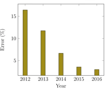
The development of convolutional neural networks (see Section 3.3) is rapidly improving every year, a good example of this can be seen by looking at the winners for the ImageNet challenge for the last years. Figure 1.5.1 shows how the winners in the classification category performed over the last 5 years, with last years winners Trimps-Soushen’s model achieving a 2.99% top-5 error. A trend which many of the newer models follow is that the models are becoming deeper. AlexNet (winner of ILSVRC2012) is built up by five convolutional layers and three fully connected layers, with the winners of 2015 presenting one ensemble of 152 layers[42].
The convolutional neural networks are also used to achieve state of the art and groundbreaking results in different applications. In [56], the authors utilized CNNs for the image question answering task, and are able to answer questions such as:What is the largest blue object in this picture? and How many pieces does the curtain have?
The authors of [53] are utilizing convolutional networks for detecting extreme weather in climate data sets. A task which normally requires human exper-tise in defining events based on physical variables, but is now achieved with convolutional neural networks with an accuracy between 89−99%.
2012 2013 2014 2015 2016 5 10 15 Year Error (%)
Figure 1.5.1: Improvement of the top 5 error for the classification task of the ImageNet challenge over the years.
1.6
Paper Outline
The outline of the rest of the thesis is the following: Chapter 2 covers the performance metrics sought in the the experiments as well as a more in depth explanation of the performance tools utilized.
Chapter 3 describes the deep learning techniques utilized in obtaining the aforementioned performance metrics.
Next, Chapter 4 explains the techniques, together with the software and hard-ware, used for the experiments.
Chapter 5 presents the experiments performed and their results in a flowing fashion.
Finally, conclusions and a discussion together with recommendations for future work are given in Chapter 6.
2 Performance Evaluation
An introduction to performance evaluation for HPC systems was given in Sec-tion 1.2. This chapter will give a more thorough explanaSec-tion of the concepts used in this thesis. First the performance metrics used in this work are intro-duced, followed by a more detailed introduction to the performance tools this work are utilizing.
2.1
POP Performance Metrics
The pursuit of optimizing performance of a parallel code can be an intimi-dating task, and it is often hard to know where to start. The communication pattern for the application might be inefficient? Or perhaps the computational distribution is not very well divided? To provide guidance for questions like these POP has defined a methodology for analysis of parallel codes, which pro-vides a quantitative measurement of the relative impact of the factors inherent in parallelisation[17].
The POP methodology is using a hierarchy of metrics where each metric rep-resent a common cause of inefficiency for parallel programs. The metrics make it possible to compare the parallel performance across different scenarios (e.g. different core counts, different input, etc.) to identify potential weaknesses of the code. The metrics are calculated as efficiencies in the range between 0 and 1, where a higher number indicates a better efficiency (which also can be pre-sented as a percentage 0−100%). As a general guideline, an efficiency above 0.8 can be regarded as acceptable, whereas values lower than that indicate performance issues where a deeper look is needed.
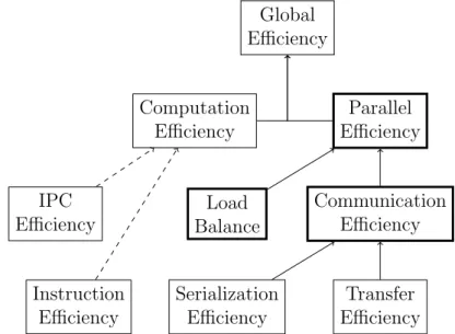
The hierarchical structure of the metrics can be seen in Figure 2.1.1. At the very top is theGlobal Efficiency which can be used to assess the overall quality of the parallelisation of the application. There are typically two main causes of inefficiencies in parallel applications, which lead to the next level in the hierarchy.
The Global Efficiency is calculated by taking the product of the Computation Efficiency and Parallel Efficiency. The Computation efficiency metric repre-sents how well the application is scaling and is calculated by computing the total time spent performing useful computations1 across all processes. In a
strong scaling scenario the sum of the useful computation time should be the same at all scales for a perfect efficiency. Two possible causes for poor Com-putation Efficiency are that dividing the work increases the total amount of computations required, and that the use of additional processes lead to con-tention on shared resources. These can be examined through the Instruction Efficiency and IPC Efficiency, respectively. Whereas they do not directly make up the Computational Efficiency, they can provide good insight.
Global Efficiency Parallel Efficiency Computation Efficiency Communication Efficiency Load Balance Transfer Efficiency Serialization Efficiency Instruction Efficiency IPC Efficiency
Figure 2.1.1: Hierarchical structure of the POP metrics, with directly af-fecting dependencies shown with whole arrows, and indirect dependencies with dashed arrows. The three metrics impor-tant for this thesis are shown in bold.
The Parallel Efficiency exposes the inefficiencies caused by dividing the work-load over processes and then communicating in between them. Similarly to the Global Efficiency, the Parallel Efficiency is defined as the product of two metrics lower in the hierarchy. In this case those metrics areLoad Balance and Communication Efficiency. The Load Balance tells how good the distribution of the workload is, and is calculated as the ratio between the average time each processor is performing useful work and the maximum time.
LoadBalance=
Pn
p=1(U sef ulComputationT imep)/n
M AX(U sef ulComputationT imen)
(2.1) The Communication Efficiency identifies applications which suffer because they spend too much time communicating, instead of performing useful work. The communication efficiency is defined as the ratio between the processor spending the most time performing useful work and the total runtime.
CommunicationEf f iciency= M AX(U sef ulComputationT imen)
T otalRuntime (2.2)
From the Communication Efficiency metric it is possible to compute two sub-metrics which breaks it further down. The sub-metrics are Serialization Efficiency and Transfer Efficiency, but to derive these metrics a simulation of an ideal network2 is required. By comparing the total runtime on a simulated ideal
network and the real network we can measure the inefficiencies due to data transfer, which is quantified with the Transfer Efficiency metric. Once the Transfer Efficiency is calculated, it is straight-forward to compute how much of the communication inefficiency comes from processors waiting for other pro-cessors to be ready to communicate. This is computed by dividing the Com-munication Efficiency by the Transfer Efficiency, and is finally quantified in the Serialization Efficiency metric.
2.2
BSC Tools Parallel Performance Analysis Suite
While there exist different tools for performance evaluation, in this thesis the tools from BSC tools[4] are used. The main tools used during this work include: Extrae - for creating trace files; and Paraver - for visualizing and obtaining metrics form the traces.
2.2.1 Extrae
The Extrae package is devoted to generating the trace files of the applications which is later used by Paraver and Dimemas3. Extrae is able to intercept calls
to parallel runtimes, such as MPI, and creates a sequence of time stamped records, which are collected in a trace file for post mortem analysis. Extrae can also capture when and where entries and exits to parallel runtimes occur, at nanosecond precision and with minimum overhead. Extrae can capture much more information than that, such as IPC and cache misses (by utilizing PAPI counters[5]), who communicates with who, and from where in the code a certain call was made. For this thesis the above mentioned features will suffice. The trace files generated are made up of three types of records:
State: A record which associates a state value for a thread during a certain time interval. Paraver is not associating any semantics to the encoding of the state field, allowing for great flexibility to take on any value. Examples of state values are; Running - the thread is performing normal computations; Waiting
2In an ideal network the communication occurs instantly.
3Dimemas - a simulation tool to answer ”what if” questions. Will not be used in this
- the thread is idle, waiting for some criterion (e.g. waiting for other threads to reach a barrier); Not yet created - the thread is not included in the set of working threads (e.g. in the beginning of an application before the master thread has created its slaves).
Event: A record representing a punctual event occurring at a certain time for a specific object. Just as for the state record, Paraver is not associating any semantics to this record, and they are simply encoded as two integers, type and value. Examples of events recorded by Extrae include, cache misses for different levels, instructions completed and entry/exit points of MPI routines, user functions, OpenMP parallel regions and CUDA kernels.
Relation (Communication): A record establishing a relationship between two object in two points in time. Examples for relation records include commu-nications between processes in MPI applications, movement of tasks between threads in OmpSs applications, and memory transfers in CUDA or OpenCL applications.
2.2.2 Paraver
Paraver is a visual API, a browser, for traces generated with Extrae. Key features in the design of Paraver were: expressive power, flexibility and ca-pability to efficiently handle large traces. The modular structure of the tools helps achieving this goal.
Two of the main design choices on which the analytic power of the tool stand on are its lack of semantics and hardwired metrics. Not having fixed semantics allows for extending the tools to support new performance data or program-ming models without any requirements of changing the visualizer, capturing it in a Paraver trace is enough. In a similar fashion, with the metrics not being hardwired, but instead programmed, a huge number of metrics may be displayed. To compute the metrics the tool offers a large set of time functions, a filter module as well as a mechanism which allows for combining two time-lines. Any metrics once computed can easily be saved in configuration files which makes it as simple as loading the saved file when the metric is to be used again.
Paraver offers a minimalistic set of views, with the philosophy that, differ-ent views should provide qualitatively differdiffer-ent types of information. The two views available are a timeline view and a statistical view. The timeline view represents the behavior along time and processes, with each window displaying a single view; a piecewise constant function of time. The types of functions displayed fall into three groups; Categorical, Logical, and Numerical. The cat-egorical functions show things such as, in which state the thread is in. The categorical functions take on an integer value [0, n] (where n is a small num-ber). The logical functions display information such as, whether the thread is in a specific user function or MPI call. The logical functions are mapped to the
set {0,1}. Finally, the numerical functions display things like the duration of an MPI call, or the number of cache misses. The numerical functions can take on any real value. An example of a timeline view can be seen in Figure 2.2.1. The functions can be represented in different ways in the views, where two of the most common ways are color encoding (where each functional values is represented with an individual color) and Not null gradient (where the func-tional values are represented according to a gradient scheme with low values taking a light green color and high values a dark blue color. Zero values are represented with a black color).
Figure 2.2.1: Paraver timeline view, with the different threads showing on the y-axis and time on the x-axis. The different colors represent different states of the application.
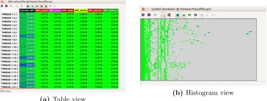
The statistical view provides numerical analysis of the traces. The statistical view can be illustrated as both tables and histograms (both in 2D and 3D), Figure 2.2.2 shows an example of both a table view as well as a histogram view. The table view allows for analyzing statistics for specific categorical control val-ues (such as different MPI calls, or different user functions). Relevant statistics to display include time (in seconds or percentage) spent in each call, number of calls, average duration of calls, etc. The histogram view displays bins of numeric control values. Each bin represents a range of values, which allows for an analysis providing insight on things such as how many instructions the different computation bursts perform for different threads, which IPC value is most common, etc.
(a) Table view
(b) Histogram view
With trace files potentially being fairly large, Paraver offers different manip-ulation methods for reducing the data down to a more manageable size. The traces can befiltered, only keeping the relevant data. Such filtered traces could, for example, be generated such that it only shows computations larger than a certain threshold, or only showing runtime related calls (removing informa-tion about hardware counter, etc.). A feature for cutting the traces exists as well, keeping all information but only for a certain time interval, or for certain processes. Typical reasons for cutting the traces are: removing initialization and finalization periods (typically not of interest) and for analysis of local behaviors not globally representative.
The Paraver kernel also provides a non-graphic interface,Paramedir. Paramedir can read traces, apply standard configurations and write a human readable ASCII output. The non graphical version is very useful in scripts and batch processing.
2.3
Analysis Process
Many applications tend to have a repetitive behavior, and often a few itera-tions are doing a good job at representing the global behavior of an applica-tion (though within each iteraapplica-tion there might be many regions with separate behaviors). Reducing the traces to fewer iterations could then significantly increase the manageability of the traces while still providing a representative analysis. Something which is exploited in this work, by fitting one iteration into a single timeline view.
The initial search space for the analysis would then be the metrics defined in Section 2.1. Once the fundamental factors for the performance have been identified, a deeper analysis can be made towards finding causes for any inef-ficiencies.
3 Deep Learning
This chapter introduces some basic background knowledge needed, for the un-familiar reader, to understand the concepts used in this thesis. This chapter begins by introducing some basics about neural networks, followed by expla-nations on the training process, and ends with covering convolutional neural networks.
3.1
Neural Networks
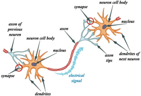
Neural networks, under which deep learning falls, have taken its inspiration from the human brain, which can be described as a biological neural network. The principles embraced are how the brain is able to process information and train itself. Much about the human brain remain a mystery, but the computer scientists work on the understanding that the brain works by having neurons collecting signals from other neurons through a number of fine structures called dendrites. The neurons are sending out electrical activity of different strengths along an axon, a long thin stand. The axons then splits to thousands of small branches, at the ends of which there is a synapse. The synapse takes the activity coming from the axon and converts it into an electrical effect, which can then either excite, or inhibit the connection to the receiving neurons. Would the inputs to a neuron be excitatory large enough compared to its inhibitory input, the neuron would ”fire” and electrical activity down its axon. Figure 3.1.1 illustrates this concept. The learning process then consists of altering the effectiveness of the synapses, in such that the influence of a certain neuron on another changes.
Neural networks have many noteworthy characteristics, which make them an attractive solution for machine learning. Their curious ability to be able to take complicated or imprecise data and obtain meaning from it, is very useful when trying to identify patterns and trends which would otherwise be too complex for a human or more conventional computer techniques to see. Furthermore, its ability to learn how to perform tasks based on the data given and to create its own representation and organize what it has learnt are all advantages which are appealing for machine learning.
Figure 3.1.1: Illustration of how the communication between neurons oc-cur.1
3.1.1 Artificial Neural Networks
The artificial equivalent of the biological neuron was first mathematically de-fined in 1943 by Warren McCulloch and Walter Pitts, and is known as the McCulloch-Pitts-Neuron, or MCP neuron[57]. The MCP neurons work un-der certain assumptions which can be summarized with the McCulloch-Pitts output rule: Ni = ( 1 P jW Nj ≥θ AND no inhibition 0 otherwise (3.1)
and visually in Figure 3.1.2. The rules say that each neuron is a binary device with a fixed threshold, theta. That the weights (W) of the excitatory inputs are all of identical weight and how the inhibitory input possesses the absolute veto over all excitatory inputs.
Output
θ
Inhibitory input Excitatory input WNj
WNk
Figure 3.1.2: Illustration of the McCulloch-Pitts output rule.
While the MCP neuron was an important definition as it introduced how neuron-like elements could execute, it had no learning capabilities, so it was
1Image from
http://www.mysearch.org.uk/website1/html/106.Connectionist. html.
basically a hard coded device. The next major stepping stone came in 1958, with the introduction of the Perceptron, which is similar to what we are using today[64]. There are some important differences between the perceptron and the MCP neuron. The weights and thresholds for perceptrons are not all identical, and the weights can take-on both positive and negative values. The inhibitory synapse is removed, but most important of all, the perceptron has got a learning rule. The perceptron can be defined as
Ni = ( 1 ui >0 0 ui ≤0 (3.2) where ui = X j WjNj+θj (3.3)
as well graphically in Figure 3.1.3, with Wj,Nj and θj being the weight, input
and bias of input neuron j, respectively.
I1 I2 ... Ij ui Wij +θ 0 input output ui 1 0
Figure 3.1.3: Illustration of the behavior of a perceptron. A neuron ui
takesj inputs, sums them together and adds a biasθ. If the result is higher than a threshold, 1 is returned, otherwise 0. The learning schema for the perceptron fairly is straightforward. Let δ be the difference between the desired target and the output (N) of the perceptron for a given input. Then the change in the weight is chosen such that it remains proportional to delta. For a certain learning rate 0< < 1, we then have:
3.1.1.1 Feed-Forward Neural Networks
The most basic use of a perceptron would be to have two inputs and a single output, which could, for example, classify which of the inputs is larger. This is an example of a single-layer feed-forward neural network (like Figure 3.1.3 illustrates), where the information is only flowing in one direction, different from recurrent neural networks2 where the information can flow backwards
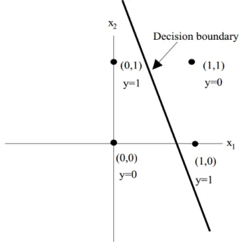
too, recurrent neural networks will not be further mentioned in this thesis. Single-layer perceptrons can have more than just two input and a single out-put. They can have an arbitrary number of both and can be used for linear regression. Though the single-layer perceptron is only able to distinguish lin-early separable pattern, illustrated in Figure 3.1.4, and in 1969 it was shown that it was incapable of learning an XOR-function3[59].
Figure 3.1.4: Limitations of the single-layer perceptron.4
The shortcomings of single-layer neural networks can be addressed with multi-layer neural networks which adds one, or multiple, extra layers between the input and the output layers. These extra layers are referred to as hidden layers. Figure 3.1.5 illustrates a multi-layer feed-forward network with one hidden layer. In fact, in 1989 it was showed in the first version of the universal approximation theorem that a feed-forward network with only a single hidden
2Recurrent neural networks create an internal memory as connections creates cycles,
something which makes them very useful for processing sequences of inputs for tasks such as, speech recognition, translation and self-driving cars.
3Exclusive Or (
⊕): a⊕b= (a∨b)∧ ¬(a∧b)
4Image from
http://www.cs.nott.ac.uk/~pszqiu/Teaching/G53MLE/ffnets-note. pdf.
layer could approximate any continuous function f ∈R, although it mentions nothing about its learnability[43].
x1 x2 x3 ... xi y1 y2 y3 ... yj z1 z2 z3 ... zk x1 x2 x3 xi z1 z2 z3 zk
Input Layer Hidden Layer Output Layer
Figure 3.1.5: Illustration of a multi-layer feed-forward neural network with i neurons in the input layer, j neurons in the single hidden layer, and kneurons in the output layer.
3.1.1.2 Activation Functions
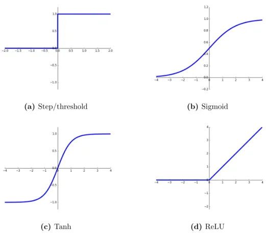
The original MCP neuron defined the output as one if a certain condition was met and zero otherwise. That is, the MCP neuron activates if a certain condition is met, according to its activation function. The MCP neuron had only a single activation function defined, namely the step/threshold function, see Figure 3.1.6(a).
But since the MCP neuron a number of activation functions have become popular. The activation functions provide a crucial role in the neural networks as they add non-linearity to the networks, without which none of the complex task could be solved. Different activation function posses different properties making some more suitable than others. The historically most popular one is the sigmoid non-linearity, which can be expressed as:
σ(x) = 1/(1 +e−x) (3.5)
and illustrated in Figure 3.1.6(b). The sigmoid function takes on values ”squeezed” into the range [0,1], where very large negative numbers takes on zero and large number takes on one. This was a nice interpretation of how the firing rate of a biological neuron was perceived to behave. Though in practice it has some major drawbacks which make them impractical during training (training explained in Section 3.2), something which has lead to them rarely ever being used any longer.
(a)Step/threshold (b) Sigmoid
(c) Tanh (d) ReLU
Figure 3.1.6: Illustrations of different activation functions.
A non-linearity which deals with some of the drawbacks of the sigmoid is the tanh non-linearity. A tanh neuron is actually just a scaled sigmoid neuron which maps the input to a number in the range [−1,1], which actually solves one of the big issues of the sigmoid, and for that reason it is in practice always preferred over the sigmoid. Tanh can be seen in Figure 3.1.6(c) and can be expressed as
tanh(x) = 2σ(2x)−1. (3.6) Though the most popular activation function the last few years has been the ReLU (Rectified Linear Unit) which simply thresholds the input at zero
f(x) =max(0, x), (3.7)
as illustrated in Figure 3.1.6(d). The ReLU non-linearity solves the big com-mon issue with the tanh and sigmoid, namely the problem with vanishing gradients5, and is also significantly faster, as no expensive computations are
needed (exponentials, etc.). Though the ReLU neuron is not without its issues,
5A well known problem, where the gradient for the earlier layers become so small, where
it turns out that it is fairly brittle during training. A large enough gradient flowing through a neuron can cause updates in such that they never will change again, and in effect ”dying”. One may find that as much as 40% of the neurons are ”dead”[7].
There are multiple attempts to deal with the dying ReLU problem, with vary-ing success, such as, settvary-ing a roof, Γ, on the output:
f(x) = max(0, min(x,Γ)), (3.8)
or like the CReLU which concatenates a positive and a negative ReLU:
ρc ,(max(0, x), max(0,−x)), (3.9)
or the leaky ReLU, which allows negative values too, though only at a fraction (α) of the magnitude of the positive ones:
f(x) =
(
x x≥0
αx x <0 (3.10)
3.2
Training
The feed-forward networks described have shown good results on many tasks, but for them to perform adequately their weights need to be properly set. The original MCP neuron required manual definition of the weights. Though this can now be done through a training step, where the model learns appropriate values for the weights.
3.2.1 Error Quantification
For the network to be able to learn, a way to quantify how good/bad a network performs is needed. This is done by defining a loss function suitable for the task in question. There are a number of different loss functions, both for classification problems and for regression problems.
Classification problems try to determine to which class a certain data belong to. This could be, for example, to determine whether an animal is a dog or a cat. Some popular loss functions for classification problems include the Softmax classifier and theSigmoid classifier. The Softmax classifier calculates a probability distribution for the classes as the following equation shows.
Si =
efyi
P
jefj
Equation (3.11) normalizes the class scores f to fit in the range 0-1. Softmax is typically used together with cross-entropy to then get a sense of how ”off” this prediction is from the ground truth. With the probability distribution vectorS and the ground truth one-hot encoded6 label vectorLwe then define
the cross-entropy loss as:
C(S, L) = −X
i
Lilog(Si). (3.12)
Whereas the classification problems try to put the input into a certain cate-gory, the regression problems are trying to predict a real-valued quantity. It could be, for example, the price of a house. For regression problems, it is common to compute the difference between the predicted values f and the ground truth y. The L1 norm or the L2 squared norm would then measure on differences. As will be explained in subsection 3.2.2 it is common to compute multiple examples in one ”batch”. One would than take the mean error over all examples, so for the mean L2 squared norm that would then be:
¯ L2 = Pn i=1(fi−yi) 2 n (3.13)
which also goes under the name, mean squared error (MSE).
3.2.2 Backpropagation
The backpropagation phase of neural network is where the actual learning oc-curs. In backpropagation, the error of the predicted output is calculated, and then propagated backwards through the network, hence the name backpropa-gation.
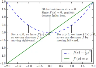
The goal of the backpropagation is to tune the weights in such a way that the loss function is minimized. This is achieved by taking the derivative of the equations in the model and following the gradient in the direction which minimizes the error. This method of following the gradient to minimize a problem is called gradient descent; a simple example of its usage can be seen in Figure 3.2.1. This work will not go into details on how gradient descent works, for more detailed explanation the reader is directed to [40].
Something which separates machine learning algorithms from the general opti-mization algorithm is that the objective function is typically made up of a sum over the training data. There are different approaches to manage this, where the straightforward thing would be to compute the gradients for all train-ing data in each traintrain-ing step, an approach called Batch Gradient Descent. Whereas computing the gradient for the entire training set would certainly
6In a one-hot encoding, a vector with as many elements as there are classes have one zero
Figure 3.2.1: Example behavior of gradient descent.7
lead to the most correct update, these computations are very costly and it has been shown that the improvements in the calculated gradients are far from linear with the increase of data used during the calculations.
Another approach would then be to only utilize a single training example per step, a method called Stochastic Gradient Descent (SGD). SGD might be the method which gives most value for each computation, though it could lead to very abrupt changes when encountering outliers. It is also unable exploit the parallel capabilities provided by GPUs, a parallelity which has been vital in the recent popularity of neural networks.
Instead the most common approach is to use a small, randomly sampled, subset of the training data for each training step, a method known asMini-batch Gra-dient Descent. The number of training images chosen for each training step, the batch size, will vary widely, but are driven by the following considerations[40]:
• Larger batch sizes will result in a more accurate gradient estimate, though with less than linear returns.
• GPUs tend to be underutilized by very small batches, leading to a min-imum batch size below which no reduction in time will be witnessed by reducing the batch size.
• The memory requirements tend to scale with the batch size, and is often the limiting factor for GPUs when increasing the batch-sizes.
• Some architectures show improved performance when choosing batch-sizes as powers of two.
While the gradient descent strategy is a popular one for optimization, it can be slow. To speed up the learning, a technique called momentum[61] could be added. The momentum algorithm uses past gradients to calculate an expo-nentially decaying moving average and continues to move in its direction. The concept of momentum is illustrated in Figure 3.2.2.
Figure 3.2.2: An example of the behavior of the momentum technique, with the black arrows showing the gradient, and the red lines the path taken when momentum is added.8
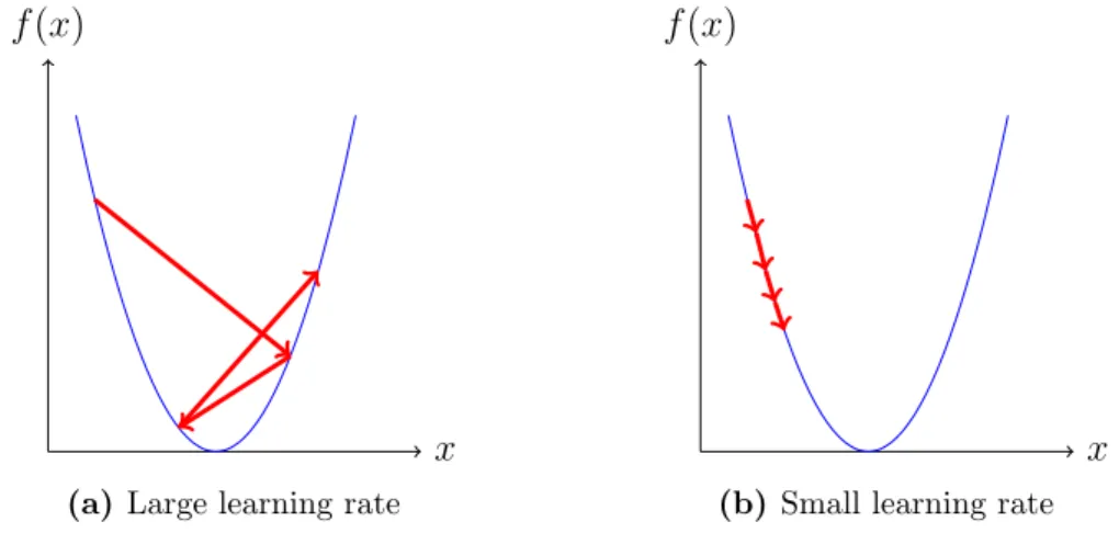
A final concern when backpropagating through the network is how big of a change to make to the weight, that is, what should the learning rate be? Too large learning rate and we might never converge, too small learning rate and it might take very long time converge (see Figure 3.2.3).
x f(x)
(a)Large learning rate
x f(x)
(b) Small learning rate
Figure 3.2.3: Illustration of the problem of choosing the correct learning rate. Too high and it will never converge, too small and it will take too long time.
An approach to manage this issue is by having an optimizing algorithm with adaptive learning rate. One such algorithm is theAdam Optimizer[48]. Adam
(formally described in Algorithm 1) calculates adaptive learning rates for each parameter and updates them individually. Similar to themomentumtechnique it keeps an exponentially decaying average of the past gradients m, and in addition, it stores the exponentially decaying average of past squared gradients
v. m and v are estimates of the first and second moments (the mean and uncentered variance) of the gradients and are used the update the weights θ, based on the initial learning rateusing the following (simplified) update rule:
θt+1=θt−
m
√
v. (3.14)
There are other optimization algorithms with adaptive learning rates, such as Adadelta[76],RMSprop[18] andAdagrad[32]. Exactly which learning algorithm to use is still unclear, but it has been shown that algorithms with an adaptive learning rate perform fairly robust over a wide range of tasks[67].
Algorithm 1 Adam Optimizer Algorithm
1: Input: Step size
2: Input: Exponential decay rates for moment estimates, ρ1 and ρ2 in [0,1). 3: Input: Small constant forδ for numerical stabilization
4: Input: Initial parameters θ 5: procedure Train(, ρ, δ, θ)
6: Initialize 1st and 2nd moment variabless = 0,r= 0
7: Initialize time stept = 0
8: while stopping criterion not metdo
9: Sample a minibatch ofm examples from the training set
{x(1), ..., x(m)} with corresponding targetsy(i). 10: Compute gradient: g ← m1∇θ
P
iL(f(x(i);θ), y(i))
11: t←t+ 1
12: Update biased first moment estimate: s←ρ1s+ (1−ρ1)g
13: Update biased second moment estimate: r←ρ2r+ (1−ρ2)gg 14: Correct bias in first moment: ˆs← 1−sρt
1
15: Correct bias in second moment: ˆr ← 1−rρt
2 16: Compute update: ∇θ=−√sˆ ˆ r+δ 17: Apply update: θ ←θ+∇θ 3.2.3 Weight Initialization
Before the training can begin, the weights in the network need to be initialized to some value. Without any knowledge on what the final values should be, it would be reasonable to assume that half of the values would be positive, and half negative. Something sounding reasonable would then be to initialize all weights to zero, which could be expected to be ”the best guess”. Though this would be an error, since this would lead to all neuron to compute the same
output, something which would also lead to them computing the same gradient during the backpropagation, and thus undergoing the same changes. To solve this, some type of symmetry breaking will be needed. Something which can be achieved by choosing small random numbered, centered around zero and with unit standard deviation (e.g. from a Gaussian) as initial values for the weights.
A problem emerging with this approach is that the variance grows with the number of inputs, and ideally the variance should remain the same for each layer. This can be achieved by utilizing the Xavier initializer[37], where the variance is set to 1/N, with N being the number of input neurons.
3.3
Convolutional Neural Networks
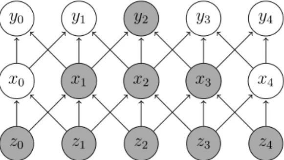
While there are a number of different classes of artificial neural networks, when it comes to image processing, convolutional neural networks (CNNs) are the most popular ones. CNNs are very similar to ordinary Neural Networks, they have weights and biases which are learnable. They have some non-linearity introducing element and in the end will predict a class score or some real value. What makes CNNs different is their assumption that the input data has a grid-like topology, such as with images.
As described earlier, and seen in Figure 3.1.5, in regular NNs all neurons in one hidden layer is connected to all neurons in the next hidden layer. It is clear to see that, with a normal sized image of 200x200 pixels and three color channels, resulting in 1200000 weights, the amount of parameters as more
neurons are added will become overwhelming. Instead, what the CNNs do is taking advantage of correlations in the neighborhoods of features, which allows for a significant reduction in the number of parameters, without reducing the performance. Two main ideas leveraged by CNNs are sparse interactions and parameter sharing.
As mentioned earlier, having fully connected neurons when images become larger (thousands or even millions of pixels) is not desirable. CNNs utilize sparse interactions by making the kernel smaller than the input image. This can be done as, even though the entire image may contain millions of pixels, meaningful feature such as edges, can be found with kernels of only tens or hun-dreds of pixels. Figure 3.3.1 illustrates the difference between fully connected and sparse interactions. This approach allows for a reductions of parameter of many orders of magnitude. Looking at Figure 3.3.2 it can be seen how, in deep networks, neurons in deeper layers can be connected, indirectly, with a larger part of the input.
The parameter sharing idea refers to idea of reusing the parameters in more than just a single place in a model, which is the case for the normal neural networks, where each element is used in a single multiplication, and then never
x0 x1 x2 x3 x4
y0 y1 y2 y3 y4
x0 x1 x2 x3 x4
y0 y1 y2 y3 y4
Figure 3.3.1: Difference between sparse connections and fully connected. As seen, a lot less connection are formed for the sparse con-nected one.
z0 z1 z2 z3 z4
x0 x1 x2 x3 x4
y0 y1 y2 y3 y4
Figure 3.3.2: In deep architectures, even with sparse connections, a large part of the input can interact indirectly with deeper neurons.
revisited again. This is a quite logical idea, as if a kernel was used to identify a vertical edge at a certain location, that same kernel would be able to identify edges at other locations as well.
3.3.1 The Convolution Layer
In the convolution layer, a certain numbers of kernels of varying size (both dependent on the architecture used) move over the image performing a dot-product and reducing the sum which produce a single output per kernel (known as feature maps). The movement of the kernels and its operations are nicely illustrated in Figure 3.3.3. Each kernel creates a feature map which could be, depending on the the usage of padding or not, and the stride used, either the same size as the input or, more commonly, smaller. The stride determines how many steps the kernels should move between the calculations, a stride of two would roughly half the size of the image. Adding padding to an image entails adding a frame of zeros to the image. This is done in some architecture to make sure that each element of the kernel reaches all parts of the image.
(a) Movement of a kernel across the feature maps/ images
(b) For each step, the kernel is multiplied with the input and the sum will make up the out-put.
Figure 3.3.3: Behavior of a kernel in a convolutional operation.11
Each of the kernels reacts to different features, at lower levels these could be things like edges or colors. Whereas the later layers react on combinations of previous layer which could be things like eyes, feet, etc. Figure 3.3.4 shows the filters learned in the early layers by Krizhevsky et. al. in the famous AlexNet9.
Figure 3.3.4: Illustration of the filters learned in AlexNet. Some are re-sponsive of certain colors, others by certain structures.12
3.3.2 Pooling Layer
It is common to introduce a pooling layer occasionally between the convolu-tional layers. The pooling layer’s main task is to reduce the dimensionality of the data, and is also useful for reducing noise and overfitting. One can describe the idea with the pooling layer by clarifying how, if one wants to identify a
9Winning architect of the 2012 ImageNet challenge. 11Image from [7].
face in an image, the pixel-wise precision on where the eye is located is not needed, merely if it is on the left or right side of the face would suffice. The pooling layer works by a kernel of a specific size which moves over the image (similar to the convolutional layer) and performs some type of pooling operations; the most popular ones are average pooling and max pooling. A very nice visual example of the downsampling of a 224x224 image using max pooling can be seen in Figure 3.3.5.
Figure 3.3.5: Example of a max pooling operation with a 2x2 kernel with i stride of two, which downsamples the image from 224x224 to 112x112.10
Whereas having some pooling layers in the architecture is still the most popular approach, there are arguments that the pooling layers should be removed, in favor of extra convolutional layers[70]. As seen earlier, this can be achieved by increasing the stride in the convolutional layers, which in effect reduces the dimensionality.
3.3.3 Example Architecture
The main building blocks of convolutional neural networks have now been introduced; an example architecture using these building blocks can be seen in Figure 3.3.6 which depicts the architecture of LeNet-5[52].
LeNet-5 is a CNN architecture designed for digit recognition. The model takes a 32x32 grey-scale image as input and passes it through a series of seven layers, to finally receive an prediction [0-9]. It consists of two convolutional layers; the first generating six feature maps of 28x28 pixels, by using a 5x5 kernel. The second convolutional layer also uses 5x5 kernels, but are producing 16 feature maps of 10x10 pixels. After each of the convolutional layer there is a sub-sampling (pooling) layer, which reduces the dimensionality to one fourth. After the second sub-sampling, three fully connected layer are added, which perform the classification based on the features extracted by the previous layers. The fully connected layers behave like the original neural networks, where all neurons are connected to all others.
Figure 3.3.6: Illustration of the LeNet-5 architecture.11
3.3.4 Transfer Learning
Deep neural networks have one big flaw; they are fairly hard to train. Typically huge amount of data and a decent amount of compute power are needed. In fact, it has become less and less common for people to train their own model from scratch, i.e. with randomly initialized weights. Instead it is more common to pre-train the model on a very large data set (such as ImageNet with 1.3 million images) and then utilize the trained model, either as a fixed feature extractor or as initial weights for later fine-tuning. Andrew Ng12claims
that transfer learning will be the next driver of machine learning’s commercial success[24]. this is possible due to the interesting phenomenon that the features extracted in the earlier layers tend to be useful for other applications as well. A feature map trained to identify a straight line trained on cat recognition will still be useful when trying to identify birds[75].
Whereas utilizing a large data-set to pre-train the network is helpful when only a small data set for the task at hand is available, general difficulties of training deep neural networks remain. A much quicker way is to use an already pre-trained model made publicly available13 and adapt the final classification
or regression to fit the problem in hand, and to keep the earlier stages of the model fixed.
11Image from [52].
12Chief scientist at Baidu and professor at Stanford.
13For example, Model Zoo[3] has multiple pre-trained models available for other people
4 Methods
In this chapter the methodologies and techniques, as well as software and hardware used in this thesis are described.
4.1
Software
For obtaining the training data the BSC performance tools with Paraver and Extrae (as introduced in Section 2.2) will be used.
For generating, and preprocessing (Section 4.4.1) the training data from the Paraver trace files, no special software was used. A simple combination of bash scripts and python code with common libraries (e.g. NumPy1 and Matplotlib2)
were used.
When it comes to software for the deep learning model there are quite a few to choose from, such as: Caffe[46], Theano[73], Torch[30] and scikit-learn[60]. But for this thesis Tensorflow[28], the open source Google developed scalable machine learning library is used.
Tensorflow was released in November 2015 and has quickly gained popular-ity. It is now one of the most popular deep learning libraries and has over 180000 commits on GitHub3. In Tensorflow, machine learning algorithms are
represented as computational graphs. Computational graphs (also known as, dataflow graphs) is a form of directed graphs where the nodes describe some type of computations, and the edges represent the data flowing between these operations[38]. The usage of data flow graphs allows for leveraging the par-allel computational capabilities of multi-core CPU, GPU and even multiple GPUs[36]. The data in Tensorflow is represented by tensors (by which the name came from) which are typed n-dimensional arrays, and on which the computations are performed. Once a computational graph has been defined, it must be launched in a Session, which places the graph onto a CPU or GPU and provides the methods to run the computations.
1NumPy: Fundamental package for scientific computing in Python,
http://www.numpy.org/
2Matplotlib: Python plotting library, producing publication quality figures,
https://matplotlib.org/
4.2
Hardware
The computations performed in this thesis were executed on two different machines, one for training the models, and another for generating data and testing the models.
The training was done on a bullx R421-E4 server which consists of[15]:
• 2 Intel Xeon E5-2630 v3 (Haswell) 8-core processors (each core at 2.4GHz with 20MB L3 cache)
• 2 K80 NVIDIA GPU Cards
• 128 GB Main memory, 8 DIMMs of 16 GB -DDR4 @ 2113 MHz - ECC - SDRAM
• Peak Performance: 250.94 TFlops
• 120 GB SSD local storage
• 1 PCIe 3.0 x8 8 GT/s, Mellanox ConnectX-3FDR 56 Gbit
• 4 Gigabit Ethernet ports
The usage of a GPU allowed for training more models and with larger images within a time frame otherwise not feasible with just a CPU.
The image generation and testing of the model were performed on a laptop with a Intel Core i7-4600U CPU, running at 2.1GHz, and having 8GiB DDR3 1600MHz memory.
Whereas training the model on a laptop would not have been feasible, no GPU is needed for evaluating or utilizing the trained models.
4.3
Neural Network Models
In the endeavor of achieving a model which was able to predict the metrics sought after, a number of different approaches were taken, all of which were utilizing convolutional neural networks. The two main approaches for training the network were:
1. Designing own models.
While the task at hand naturally would be considered a regression problem, typicallyclassification problems are somewhat easier to train[7]. In this thesis both approaches will be explored. To achieve this, the final fully connected layer together with the loss function will be adapted for each of the two ap-proaches.
4.3.1 VGG-19
As pre-existing model, the VGG-19[68] architecture was used, although with some alterations. VGG-19 was introduced for the 2014 ILSVRC, where it won first and second place in localization and classification tasks respectively. The authors have openly released the weight used in the Imagenet challenge, which were trained on the Imagenet data set[31], containing 1.3 million images of 1000 different categories. The weights were released to the Caffe model zoo repository[3] and have later been converted to be compatible with Tensorflow models[22].
The original VGG-19 model is built up by 16 convolutional layers, as seen in Table 1, and three fully connected layers. The convolutional layers are utilizing fairly small kernels sizes of 3x3, and have set the stride and padding set to 1, which leads to the output feature maps have the same spatial dimensions as the input feature maps. For each of the convolutional- and fully connected layers ReLUs (explained in Section 3.1.1.2) are utilized to achieve non-linearity. For down-sampling of the feature maps, the convolutional layers were intertwined with max pooling layers (introduced in Section 3.3.2). The max pooling lay-ers utilized non-overlapping 2x2 kernels (i.e. stride two), which reduced the feature vector sizes by a factor of two. The full spatial configuration of the convolutional and pooling layers of VGG-19 can be seen in Table 1 and more thoroughly explained in the paper [68].
Layer Weight dimension Kernel Size Stride Size reduction factor Pooling/ Activation Data (1,1) Conv1 1 (64,3,3,3) 3 1 ReLU Conv1 2 (64,64,3,3) 3 1 ReLU
Pool1 2 2 (2,2) Max Pooling
Conv2 1 (128,64,3,3) 3 1 ReLU
Conv2 2 (128,128,3,3) 3 1 ReLU
Pool2 2 2 (4,4) Max Pooling
Conv3 1 (256,128,3,3) 3 1 ReLU
Conv3 2 (256,256,3,3) 3 1 ReLU
Conv3 3 (256,256,3,3) 3 1 ReLU
Conv3 4 (256,256,3,3) 3 1 ReLU
Conv4 1 (512,256,3,3) 3 1 ReLU
Conv4 2 (512,512,3,3) 3 1 ReLU
Conv4 3 (512,512,3,3) 3 1 ReLU
Conv4 4 (512,512,3,3) 3 1 ReLU
Pool4 2 2 (16,16) Max Pooling
Conv5 1 (512,512,3,3) 3 1 ReLU
Conv5 2 (512,512,3,3) 3 1 ReLU
Conv5 3 (512,512,3,3) 3 1 ReLU
Conv5 4 (512,512,3,3) 3 1 ReLU
Pool5 2 2 (32,32) Max Pooling
Table 1: Structure of the original VGG-19’s convolutional and pooling lay-ers.
4.3.1.1 Architecture modifications
With the original VGG-19 model as a baseline, a number of alternative models were produced. For the models created for this thesis, only the convolutional and pooling layers (i.e. the feature extraction) from VGG-19 were used. Three fully connected layers were then used to produce the desired output (regres-sion/classification).
As utilizing average pooling instead of max pooling has been seen to show some improvements[35], one alteration tested was to replace the original max pooling layers with average pooling layers throughout the network. For similar reasons, tests were performed where the activation functions were changed from ReLUs to Leaky ReLUs.
The models based on the VGG-19 architecture will be referred to using the following naming convention:
VGG-19 Pooling Activation Output
Each of the parameters will take on a single letter with the following mapping:
Pooling Activation Output
Max pool Average pool ReLU Leaky ReLU Classification Regression
M A R LR C R
4.3.2 Custom Models
Apart from the VGG-19 based models, attempts at creating and training new models from scratch were also made. The custom models created were de-signed following the design principles presented in [69]. More specifically, the
design patterns which the custom models will aim at fulfilling are: to strive for simplicity, to increasing symmetry, and following a pyramid shape.
It has been shown that simple architectures with very few different types of units can perform very well[70]. Based on these findings the custom models will only consist of four types of computations; convolutions, ReLUs, average pooling, and fully connected multiply and adds.
There is also evidence of having symmetry (i.e. repeating structures) in an architecture to facilitate training of deeper networks, such as in [50]. With this in mind, the custom models will be constructed of blocks of two convolutional operations and two ReLUs, followed by an average pooling.
Block={CON V −ReLU −CON V −ReLU−AV G.P OOL}
The final design principle on which the models were based on was for the ar-chitecture to have a pyramid shape. One of the fundamental design patterns for convolutional networks is the trade-off between maximum representational power and elimination of redundant information. With the architecture hav-ing a pyramid shape refers to that there should be an overall smooth down-sampling, combined with an increasing number of channels in throughout the architecture, which is exemplified in [41]. Taking this in consideration, the number of channels added from one layer to another is kept small, and the pooling performed is only done with a stride of two, not higher.
The custom models created consist of a number n of the previously explained blocks, followed by three fully connected layers.
Architecture=Block × n−F C6−F C7−F C8
Architectures up to four blocks (n = 4) were used for the custom models. The naming convention for the custom models is the following:
Custom n, n ∈[1,2,3,4].
4.4
Data Generation
The models were trained against Paraver MPI timeline images of different traces available within the POP project at BSC. A total of 200418 images were
generated, for different core counts, ranging from 6 cores up to 48 cores, with efficiency metrics evenly divided between 0−100%.
To generate the images, a small chop4of the trace file was made using Paramedir.
The chops were then loaded with Paraver, which produced a timeline image,
similar to Figure 4.4.1, and calculated the performance metrics for that specific chop. The workflow of the data generation can be seen in Algorithm 2.
Figure 4.4.1: Example of an unprocessed training image. Different ranks are projected on the y-axis, and time along the x-axis. The different colors represent time spent in different MPI calls, with black being time outside of MPI.
Algorithm 2 Data Generation Workflow
1: procedure Generate Data(TracefileF, Time Interval Ti,j)
2: Chop ← Paramedir(F,Ti,j)
3: Image,Metrics ←Paraver(Chop) 4: Return Image, Metrics
The images generated in this process were of 200x525 pixels. Having the images being larger in width than in height allows for more detailed information about the trace in the same image.
4.4.1 Data Pre-Processing
During the work, whether pprocessing the images would produce better re-sults or not was investigated. Pre-processing the images produces two main benefits for the training. Firstly, non-relevant information in the image (such as the name of the trace) are filtered out, thus reducing the intellectual ca-pabilities needed for the model. Secondly, the dimensionality of the images is reduced, which in turn means less computations and less memory needed for the model, leading to faster convergence.
The pre-processing consists of three phases. First the black borders were cropped out of the image (See Figure 4.4.1 for example of an image before pre-processing.). Secondly, the black padding between the ranks was removed, and the timeline was re-painted with time spent within the parallel runtime in blue, and time performing useful work in green. Finally, the image was re-scaled to fit the dimensions 144x490 pixels (re-scaling the images allows for different core counts to be trained on the same model), which is about a third
(application dependent) fraction of the total execution time, resulting in a trace file with the same number of ranks, but just a small time frame.