Quantifying counterparty credit risk

(1)

Quantifying Counterparty Credit Risk

P.M. Ndlangamandla

Programme in Advanced Mathematics of Finance, University of the Witwatersrand,

Johannesburg.

(2)

Declaration

I declare that this project is my own, unaided work. It is being submitted as partial fulfilment of the Degree of Master of Science in the University of the Witwatersrand, Johannesburg. It has not been submitted before for any degree or examination in any other University.

P.M. Ndlangamandla October 10, 2012

(3)

Abstract

Counterparty credit risk (CCR) is the risk that a counterparty in a deal will not be able to meet their contractual obligations in the future. While CCR is an important task for any risk desk, it has often been underestimated due to the miss-conception that some counterparties were deemed to be either too big to fail or too big to be allowed to default. This was highlighted by the 2008 financial crisis that saw respected banks, such as Lehman Brothers, and financial service providers, such as AIG, default on their obligations. Since then there has been renewed interest in CCR, with the focus being on actively pricing and hedging it. In this work CCR is invistigated including its intersection with other forms of risk. CCR mitigation techniques are explored, followed by the formal quantification of CCR in the form of credit value adjustments (CVA). The analysis of CCR is then applied to interest rate derivatives, more specifically forward rate agreements (FRAs) and interest rate swaps (IRSs).

The effect of correlation on unilateral and bilateral CVA between counterpar-ties, including risk factors such as the interest rate, is investigated. This is in-vistigated under two credit risk modelling frameworks, the structural and intensity based frameworks. It is shown that correlation has a none-negligible effect on both unilateral and bilateral CVA for FRAs and IRSs. Correlation structures, namely the Gaussian and the Student-t copula, are used to induce dependency in order to understand their effect on both unilateral and bilateral CVA. It is shown that the choice of copula does not have significant effect on either unilateral or bilateral CVA.

(4)

Acknowledgements

I would like to thank my supervisors, Dr Thomas McWalter and Prof Coenraad Labuschagne for their patience, encouragement and effort. The long hours I spent with Tom in the final stages were the most inspirational and motivational. I would also like to thank the academics, Prof Mervyn Curtis, Prof David Taylor, Mike Mchunu and Prof Scott Hazelhurst, for all the support they gave me. Special thanks go to Rand Merchant Bank in particular Glenn Brickhill, Theo Thomas, Patrick Reynolds, Tracey Ashington and Ilka Dunne, for the moral and financial support. Glenn Brickhill was available to discuss possible research topics on a number of occa-sions and will always be responsible for my passion in credit risk modeling. I would also like to acknowledge the financial support received from the National Research Foundation (NRF) and the Mellon Foundation. I appreciate the amount of effort Mokgadi Rasekgala and Theresa Offwood-le Roux put in editing and proofreading my work. Last but not least, I would like to thank my family for their love and support in all that I have done.

(5)

List of Figures

2.1 The Student-t Copula . . . 25 5.1 Merton Vs. First Passage Time Model . . . 64 7.1 Swap Zero Curve as of 5 December 2011 . . . 92 7.2 Unilateral CVA in Swaps: Using a First Passage Time Model . . . . 101 7.3 Bilateral CVA in Swaps: Using a First Passage Time Model to model

Credit Risk . . . 103 7.4 Unilateral CVA in Swaps: Under the Intensity Framework for Credit

Risk Modelling . . . 106 7.5 Bilateral CVA in Swaps: Under the Intensity Framework for Credit

Risk Modelling . . . 107 7.6 Effect of Correlation on Default Times . . . 108 7.7 Correlation Effects on both the UCVA and BCVA when Credit Risk

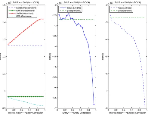
is Modelled Using a First Passage Time Model . . . 110 7.8 Correlation Effect both the UCVA and BCVA when Credit Risk is

Modelled Under the Intensity Process . . . 112

(9)

List of Tables

A.1 Pricing curves . . . 117 A.2 Calibrated Volatilities . . . 119 B.1 Standard Bank and South African Breweries in FRA Deals (Unilateral

CVA Using a First Passage Time) . . . 120 B.2 Standard Bank and Old Mutual in FRA Deals (Unilateral CVA Using

a First Passage Time) . . . 121 B.3 Standard Bank and Anglo American in FRA Deals (Unilateral CVA

Using a First Passage Time) . . . 121 B.4 Standard Bank and South African Breweries in Swap Deals

(Unilat-eral CVA Using a First Passage Time) . . . 121 B.5 Standard Bank and Old Mutual in Swap Deals (Unilateral CVA Using

a First Passage Time) . . . 122 B.6 Standard Bank and Anglo American in Swap Deals (Unilateral CVA

Using a First Passage Time) . . . 122 B.7 Standard Bank and South African Breweries in FRA Deals (Bilateral

CVA Using a First Passage Time) . . . 123 B.8 Standard Bank and Old Mutual in FRA Deals (Bilateral CVA Using

a First Passage Time) . . . 123 B.9 Standard Bank and Anglo American in FRA Deals (Bilateral CVA

Using a First Passage Time) . . . 123 B.10 Standard Bank and South African Breweries in Swap Deals (Bilateral

CVA Using a First Passage Time) . . . 124 B.11 Standard Bank and Old Mutual in Swap Deals (Bilateral CVA Using

a First Passage Time) . . . 124 B.12 Standard Bank and Anglo American in Swap Deals (Bilateral CVA

Using a First Passage Time) . . . 125 B.13 Standard Bank and South African Breweries in FRA Deals (Unilateral

CVA Using an Intensity Framework) . . . 126 B.14 Standard Bank and Old Mutual in FRA Deals (Unilateral CVA Using

an Intensity Framework) . . . 126 B.15 Standard Bank and Anglo American in FRA Deals (Unilateral CVA

Using an Intensity Framework) . . . 126 B.16 Standard Bank and South African Breweries in Swap Deals

(Unilat-eral CVA Using an Intensity Framework) . . . 127

(10)

LIST OF TABLES vi

B.17 Standard Bank and Old Mutual in Swap Deals (Unilateral CVA Using an Intensity Framework) . . . 127 B.18 Standard Bank and Anglo American in Swap Deals (Unilateral CVA

Using an Intensity Framework) . . . 127 B.19 Standard Bank and South African Breweries in FRA Deals (Bilateral

CVA Using a First Passage Time) . . . 128 B.20 Standard Bank and Old Mutual in FRA Deals (Bilateral CVA Using

a First Passage Time) . . . 128 B.21 Standard Bank and Anglo American in FRA Deals (Bilateral CVA

Using a First Passage Time) . . . 128 B.22 Standard Bank and South African Breweries in Swap Deals (Bilateral

CVA Using a First Passage Time) . . . 129 B.23 Standard Bank and Old Mutual in Swap Deals (Bilateral CVA Using

a First Passage Time) . . . 129 B.24 Standard Bank and Anglo American in Swap Deals (Bilateral CVA

Using a First Passage Time) . . . 129 B.25 Standard Bank and Old Mutual in a 5YR Swap with a R100 mill

Notional (Unilateral CVA Using a First Passage Time Model) . . . . 130 B.26 Standard Bank and Old Mutual in a 5YR Swap with a R100 mill

Notional (Bilateral CVA Using a First Passage Time Model) . . . . 131 B.27 Standard Bank and Old Mutual in a 5YR Swap with a R100 mill

Notional (Unilateral CVA Using an an Intensity Framework) . . . . 132 B.28 Standard Bank and Old Mutual in a 5YR Swap with a R100 mill

(11)

List of Algorithms

1 This algorithm returns a set of default times for each path simulated for the company value and corresponding default times . . . 94 2 This algorithm returns a matrix with each column being a path

gen-erated by the CIR++ model . . . 94 3 This algorithm returns the price of any one of the two instruments

above, if f lag = 1 then it pricesCl else it pricesb Fl withb f lag=−1 . 97 4 This algorithm returns the price of any one of the two instruments

above, iff lag = 1 then it pricesPaySwaption else it pricesd RecSwaptiond with f lag=−1 . . . 98

(12)

Chapter 1

Introduction

Counterparty risk is the risk that is specific to a counterparty in a derivatives deal. One such risk specific to a counterparty is credit risk, which is the risk that the counterparty will not be able to meet their contractual obligations. This type of risk, while not in isolation from other risks, naturally arises every time a new deal/trade is booked over-the-counter (OTC). Exchange traded contracts are also not immune from this form of risk as they are also backed by clearing members that may default. Trading OTC derivatives has the advantage that it limits the spread of information on the trades done, which guarantees that hedging and trading strategies are not unfairly copied, however, the introduction of counterparty specific risk is the main disadvantage.

The bank of International Settlements (BIS) estimates that as of the end of June 2010 the total notional outstanding for OTC trades to be well over 582 trillion dollars, more than 70% of which are interest rate swaps (IRSs) and forward rate agreements (FRAs)[37]. This signifies a growing OTC derivatives market and the growing importance of managing counterparty risk in general and more specifically managing counterparty credit risk (CCR). As already mentioned CCR does not exist in isolation of other risks. It is associated with market risk, in that, prevailing market conditions can lead to the deterioration of a counterparty’s credit quality which subsequently leads to greater exposure. Also, trading under the International Swaps and Derivatives Association (ISDA) master agreement with the credit support annex (CSA) activated is generally a CCR mitigating technique but may lead to the introduction of liquidity risk which would generally be caused by lack of buyers for the posted collateral during times of distress. Its interaction with other forms of risk indicates that in quantifying CCR, it is necessary to consider the correlation of default with other risk factors.

Counterparty risk management practices are mature, having been noted already

(13)

2

in Basel 2 [68]. Managing counterparty credit risk may involve employing techniques such as netting, close-out netting and collateral posting. All these are supported by the ISDA master agreement and will be discussed in Chapter 3 of the dissertation. A more controversial and intuitive approach would be to only trade with counterparties of the highest credit quality. This is controversial not only because it subjects small counterparties to unfair competition but also because companies with good ratings may fail — in the recent history, for example, Lehman Brothers was rated AA moments before it failed.

On another front CCR management has often been based on the calculation of credit exposure profiles for counterparties. Several metrics exist, these include amongst others Expected Exposure (EE), Potential Future Exposure (PFE), Ex-pected Positive Exposure (EPE), Effective ExEx-pected Positive Exposure (EEPE) etc. [47]. These risk metrics can be important when making decisions on which counter-parties to trade with. An institution would usually set credit lines for countercounter-parties as part of policy which would aid as a limit for the institution from doing trades with certain counterparties due to their current exposure profiles [21].

The above mentioned counterparty risk mitigation techniques are effective and the risk metrics provide much needed insight for correct decision making. However, there is one weakness inherent in them; they fail to quantify CCR. This weakness implies that they do not give a formal way of hedging the CCR. Standard pricing theory, assuming complete markets, and precluding arbitrage opportunities, informs us that the cost of hedging a contingent claim is the fair price of the contingent claim. Quantifying CCR is intuitively calculating that adjustment to a price of a derivative that assumes no CCR. In a complete market this adjustment should be enough to hedge the CCR inherent in the derivative, and is popularly known as a credit value adjustment (CVA)/expected loss (EL). There are many variants of CVA but in general there are two ways of approaching CVA:

• Unilateral: Only one counterparty is assumed to be default prone. Usually

the party calculating the CVA assumes themselves to be risk free and assumes the other party to be default prone. The motivation for this could be that the credit qualities of the two counterparties differ significantly such that the default of the highly rated counterparty is expected to occur later than the default of the other counterparty if it does occur.

• Bilateral: When the valuation is being done, both counterparties assume

themselves to be default prone. This is sometimes referred to as BCVA and has two components; one component is due to the counterparty and one due to the valuator’s own credit quality. This is usually the approach when both

(14)

3

parties are of comparable credit quality. It could also be motivated by the fact that considering the credit quality of both counterparties comes with a benefit. This benefit is known as a DVA benefit and will be explained in Chapter 3. While the motivation behind unilateral CVA may appear obvious, the motiva-tion for Bilateral CVA is less obvious. Bilateral CVA has gained popularity over recent years but its first appearance dates back to 2005 in the paper by Cheburini [23]. Studies on CVA, and counterparty risk in general, that have focused on the South African market include the work done by Milwidsky [62] and Le Roux [59]. The motivation behind bilateral CVA is, as the recent financial crisis illustrated that respected banks and financial institutions can default with positive probability. Notable examples were Lehman Brothers, Fennie Mae, Fredie Mac, Washington Mu-tual, Landsbanki, Glitnir and Kaupthing who all defaulted in the same month [12]. It is thus valid for any financial institution, regardless of its current credit rating, to also consider its own credit risk.

The bilateral nature of CCR appears when dealing with instruments such as IRSs where the instrument can be a liability to both parties, not necessarily at the same time. In the obvious case of bonds, the counterparty risk is unilateral since the borrower is the only party who remains the one with an obligation to pay the coupons and the principal up until maturity.

The dissertation proceeds as follows: in Chapter 2 we give some of the results and definitions that explain certain concepts used in the dissertation. Chapter 3 is a review of CCR management and mitigating techniques. In the same chapter several approaches to quantify CCR in the form of CVA are introduced namely, calculation from first principles, exposure profiles approach and the portfolio or value decompo-sition approach. In Chapter 4, short rate models, in particular the CIR and CIR++ models are introduced and explored with the aim of using CIR++ as a model for the short rate and intensity of a default prone entity. In Chapter 5, two credit risk modelling frameworks are reviewed, namely the intensity and the less popular structural framework. In the same chapter, descriptions of how calibration to credit default swaps (CDSs) can be achieved under both frameworks are also presented. In Chapter 6, the CVA analysis is focused on forward rate agreements (FRAs) and interest rate swaps (IRSs). The analysis results in analytic and semi-analytic ap-proximations of CVA and BCVA being derived and presented when the underlying contracts are FRAs and IRSs. In Chapter 7, algorithms for simulating default times under the two credit risk modelling frameworks are introduced and presented along with Monte Carlo algorithms for valuing the semi-analytic expressions presented in Chapter 6. Furthermore, two studies involving South African multinationals are presented, the first study presents results showing how UCVA and BCVA behave

(15)

4

for increasing tenors of both FRAs and IRSs and the second study shows how cor-relation impacts UCVA and BCVA under both credit risk modelling frameworks. The Gaussian and Student-t copula are used to induce correlation in the first study. Chapter 8 concludes the work and points to future work.

(16)

Chapter 2

Mathematical Preliminaries

This chapter is a summary of the results needed for this dissertation. It is the goal of this chapter to provide an introduction and a reminder to advanced readers, of the results that will be used in this dissertation. It is however a fair recom-mendation that advanced readers can proceed to the next chapter without loss of understanding. Good introductory references are the two volumes by Shreve [74, 75] and for advanced readers interested in all technical details, Jacod and Shiryaev is recommended [54, 5]. Furthermore, basic statistics knowledge is assumed.

Definition 2.1. Let Ω be a nonempty set, and let F be a σ-algebra of subsets of

Ω. Aprobability measure Pis a function that, to every setA∈ F, assigns a number in [0,1], called the probability ofA and writtenP{A}. We require that:

(i) P{Ω}= 1 and

(ii) whenever A1, A2, . . . is a sequence of disjoint sets in F, then the probability

of the union of disjoint events is the sum of the individual probabilities, i.e., P(∪∞n=1An) =

∞

X

i=1

P(An). (2.1)

The triplet (Ω,F,P) is called a probability space.

A probability space is used to model the whole economy in which we will be pricing instruments. We will denote the set of all events possible in our economy by Ω and the function that assigns the probabilities to each event in Ω by P.

Definition 2.2. A stochastic process, denoted by X = (Xt), t ∈ I, is a family of

real-valued random variables Xt : Ω→ R, indexed by t∈I, where I is some index set. The two cases of most interest are when I is a subinterval ofN, in which case X is called a discrete-time stochastic process; and whenI is a subinterval ofR+_{, in}

which case X is called a continuous-time stochastic process.

(17)

2.1. INFORMATION, FILTRATIONS AND STOPPING TIMES 6

We wish to model the values that are attained by stochastic processes in con-tinuous time. It is also the case that in most mathematical finance applications, a finite time horizon is considered.

Definition 2.3. For a fixed sample pointω∈Ω, the mapt→Xt(ω), fort∈R+, is

called asample path ortrajectory of a stochastic processX.

This is just the progression of values attained by the stochastic process as a function of time.

2.1 Information, Filtrations and Stopping Times

The flow of information is a fundamental idea because while available information can not in general inform us what the precise values of the fundamental variables we wish to model as stochastic processes are, it can tell us which are possible and which are not. This leads us to the notion of a filtration. Intuitively, this is a set of information that has been accumulated up to a point in time1.

Definition 2.4. Let Ω be a nonempty set. LetT be a fixed positive number, and

assume that for eacht∈[0, T] there is aσ-algebraF_t. Assume further that ifs≤t, then every set in Fs is also in Ft. Then we call the collection of σ-algebras Ft, 0≤t≤T, afiltration.

This leads to the concept of a filtered probability space. Firstly we define a P -completeσ-algebra as follows,

Definition 2.5. A σ-algebra F is P-complete if for all A ⊆ B, with B ∈ F such

that P(B) = 0, implies that A∈ F.

Definition 2.6. A probability space (Ω,F,P) is called afiltered probability spaceif it

is endowed with a filtration. The combined structure is denoted by (Ω,F,(Ft)t≥0,P). For convenience we will denote (F_t)t≥0 byFt.

Definition 2.7. A probability space (Ω,F,P) is called P-complete if all the σ

-algebras (F_t)t≥0 and F0 contain all the P-null sets of (Ft)t≥0.

Definition 2.8. A probability space (Ω,F,P) is said to satisfy theusual conditions

if it is complete and the filtration is right continuous; i.e., Ft=Ft+:=

\

t>s

Fs, t∈R+. (2.2)

(18)

As a random variable takes certain values in time, it generates information, i.e., it generates a filtration and below we state what this means in terms of our probability space.

Definition 2.9. Let X be a random variable defined on a nonempty sample space

Ω. The σ-algebra generated byX, denoted by σ(X), is the collection of all subsets of Ω of the form {ω∈Ω;X(ω)∈B}, where B are all the Borel subsets ofR.

At this point it is important to introduce several concepts that play a central role in financial modelling: measurability, predictability and previsibility.

Definition 2.10. Given a filtered probability space, (Ω,F,F_t,P) and a stochastic

process Xt, we say Xt is Ft-measurable if every set in the σ-algebra generated by Xt,σ(Xt) is in Ft.

Intuitively a random variable is measurable with respect to a given filtration if the information contained in that filtration is enough to determine its value.

Definition 2.11. Given a filtered probability space, (Ω,F,F_t,P) and a stochastic

processXt, we say Xt isprevisible if∀t,∃s < tsuch that Xt is Fs-measurable. Intuitively previsibility means that at a particular point in timetwe can tell the value of the stochastic process at time t+ ∆t precisely because of the information we have at timet.2

Definition 2.12. Given a filtered probability space, (Ω,F,Ft,P) and a stochastic

processXt. Xtis predictable if it is measurable with respect toFt.

These definitions lead to an important concept that will be used to define the notion of a stochastic integral, this concept is what is known as adaptativity,

Definition 2.13. Let Ω be a nonempty sample space equipped with a filtrationF_t,

0 ≤t≤T. LetX(t) be a collection of random variables indexed by t∈[0, T]. We say this collection of random variables is an adapted stochastic process if, for eacht, the random variable Xt is Ft-measurable.

We have already mentioned in passing the idea of stopping times and below we formalize the important types which are predictable and totally inaccessible, this is done through a series of definitions. Firstly the notion of a random time needs to be defined as follows.

2

As an example a company may announce that dividends will be paid or that there will be a sale of assets at some future date from the announcement date

(19)

Definition 2.14. Given a probability space (Ω,F,P), arandom timeis a universally

measurable function on Ω with values in [0,∞]. Using this definition we define a stopping time.

Definition 2.15. Given a probability space (Ω,F,P), a random timeτ in this space

is astopping time if{τ ≤t} ∈ F_t,∀t∈_R+_.

This means that only information up to time t is necessary to conclude on whether time τ has arrived or not. This time is referred to as an F-stopping time. We now define what a predictable stopping time is.

Definition 2.16. Given a probability space (Ω,F,P), then τ is a predictable

F-stopping time if there exists a sequence of F-stopping times {τ1, τ2, . . . , τn} such

that the sequence is increasing for all n∈_Nand limn→∞ =τ. The sequence is said

toannounce τ.

Stopping times associated with continuous processes are commonly predictable because of the continuity. To add some intuition to predictability of a stochastic pro-cess, it can be said that a stochastic process taking a particular value is predictable if prior to it obtaining that value there is a series of “stopping times” that announce that the process is going to take that value. This is associated with left-continuous processes3_{. The next concept to explore is that of accessibility of stopping times.}

Definition 2.17. Given a probability space (Ω,F,P), then τ is an accessible

F-stopping time if there exists a sequence ofF-stopping times{τ0, τ1, . . .} such that,

P{∪∞k=1{ω∈Ω :τk(ω) =τ(ω)<∞}}=P{τ <∞}. (2.3) The stopping time of interest to credit risk modelling is the one that is not accessible due to the fact that defaults are rare events and normally come as a jump or complete surprise. Below we define what a totally inaccessible stopping time is.

Definition 2.18. Given a probability space (Ω,F,P), thenτ is atotally inaccessible

F-stopping time if for every predictable stopping timeζ we have that,

P{ω∈Ω :τ(w) =ζ(w)<∞}= 0. (2.4) Intuitively the stopping time can never be announced by an increasing sequence of stopping times. The graph of a stopping time or path is defined as follows,

3

It does not mean that prior to the random variable taking that value, we are able to tell that it will take it. It means that after attaining that value there is an infinitesimal time before that time which announced it. This concept becomes more crucial in the credit risk modelling part of the thesis.

(20)

2.2. MARTINGALES AND SEMI-MARTINGALES 9

Definition 2.19. Given a probability space (Ω,F,P), then the graph of an

F-stopping time τ is {(t, ω) : 0≤t=τ(ω)<∞}and is denoted by [τ].

The following theorem states that any stopping time can be decomposed into a totally inaccessible and accessible stopping time.

Theorem 2.20(Decomposition of stopping times). For every stopping timeτ, there

exists one (up toP-negligibility) and only one pair (τp, τi) of stopping times with the

properties,

1. [τ] = [τp]∪[τi] such that [τp]∩[τi] = Ø, 2. τi is inaccessible and

3. There exist a sequence {ζ1, ζ2, . . . , ζn}, n ∈ N, of predictable stopping times

such that [τp]⊂ ∪k=1[ζk].

Proof. For the proof we refer to Metivier [61, p.28].

Stopping times introduce the idea of a stopped process.

Definition 2.21. Given a process Xt and a finite stopping time τ, the stopped

process at timeτ, denoted byXτ

t, is given by,

Xτ∧t=It<τXt+It≥τXτ, ∀t∈R+. (2.5)

2.2 Martingales and Semi-martingales

One of the most important concepts in mathematical finance is the notion of mar-tingales. They intuitively represent a fair game, in that they do not have a tendency to increase or decrease over time. We define them precisely below, but first we need to understand integrability of random variables,

Definition 2.22. Given the probability space (Ω,F,P), the family of random

vari-ablesX : Ω→R= [−∞,∞], such that,

(E [|X|p])1p ₌ Z Ω |X|pdP 1_p <∞, p≥1, (2.6) is denoted byLp_(Ω_,_F_, P).

Definition 2.23. A random variable is p-integrable if it belongs toLp_(Ω_,_F_,

P).

Definition 2.24. A process X is called uniformly integrable if it satisfies,

lim n→∞_tsup_∈ R+ Z |Xt|≥n |Xt|d_P= 0. (2.7)

(21)

2.2. MARTINGALES AND SEMI-MARTINGALES 10

Definition 2.25. A process X in a filtered probability space

(Ω,F,(F_t)t≥0,P) is a martingale if, 1. Xt is adapted toF,

2. Xt is integrable,∀t∈R+ and 3. E[Xt| Fs] =Xs,∀s≤t∈R+.

If in (3), we have that E[Xt | Fs]≥Xs, then the process is called a sub-martingale and if we have thatE[Xt| Fs]≤Xs then it is called asuper-martingale.

Definition 2.25, (3) tells us that on average, a martingale is constant at any future time. This means that there is no tendency for the value to increase or decrease. This is a central idea behind mathematical finance in that it is linked to the principle of no arbitrage which will be discussed in the section on pricing. Intuitively a super-martingale is a process that drifts down on average and similarly a sub-martingale is a process that drifts up on average. A martingale is then a process that is both a sub and super martingale. All these belong to a class of processes called semi-martingales.

Another more general class of is that of local martingales and in general all martingales are local martingales but not all local martingales are martingales.

Definition 2.26. A process Xt in a filtered probability space (Ω,F,(Ft)t≥0,P) is

a local martingale, referred to as an F-local martingale, if there exist an increasing sequence of stopping times {τ1, τ2, . . . , τn}with limn→∞τn=∞ such that,

1. Xt is adapted and right-continuous and 2. ∀i∈[0, n] the stopped processXτi

t is anF-martingale.

The sequence of stopping times is called a localizing sequence or reducing se-quence.

Definition 2.27. A processXtin a filtered probability space (Ω,F,(Ft)t≥0,P) is a

semi-martingale if it can be decomposed as follows,

Xt=Mt+At, (2.8)

where Mt is a local martingale with M0 = 0 and At is a process with locally finite

variation.

(22)

2.3. STOCHASTIC DIFFERENTIAL EQUATIONS 11

2.3 Stochastic Differential Equations

Stochastic differential equations are non-deterministic versions of ordinary differen-tial equations. The deterministic nature is eliminated due to the introduction of a noise term. We focus on SDEs of the form,

dXt=f(Xt, t)dt+g(Xt, t)dWt, given X0 =K ∈R+, (2.9) where Wt is our added noise.

The exciting history around this noise which is known as Brownian motion can be found in H¨anggi and Marchesoni [49] and we define it next,

Definition 2.28. Let (Ω,F,P) be a probability space. For each ω ∈ Ω, suppose

there is a continuous function Wt of t ≥0 that satisfies W0 = 0 and that depends

on ω. Then Wt, t ≥0 is a Brownian motion if for all 0 =t0 < t1 <· · · < tm the increments, Wt1 −Wt0, Wt2 −Wt1, . . . , Wtm−Wtm−1 are independent and each of

these increments is normally distributed with,

E[Wti+1−Wti] = 0, (2.10)

E[(Wti+1−Wti)

2_{] =}_t

i+1−ti. (2.11)

There are many important results concerning Brownian motion but one that is obvious is the following:

Theorem 2.29. Brownian motion is a martingale.

The process described by (2.9), with some conditions on the functions f(Xt, t) and g(Xt, t), are known as Itˆo processes. To be more precise, we define them below.

Definition 2.30. If Wt is as defined in Definition (2.28) then an Itˆo process is a

stochastic process of the form,

dXt=f(Xt, t)dt+g(Xt, t)dWt, given X0 =K ∈R+, (2.12)

which is shorthand for, Xt=X0+ Z t 0 g(Xu, u)dWu+ Z t 0 f(Xu, u)dt, (2.13)

whereX0is non-random andg(Xu, u) andf(Xu, u) are adapted stochastic processes.

These processes are the most popular for the modelling of financial variables and can be extended by incorporating jumps to form what is known as a jump diffu-sion process. The construction of equation (2.13) introduced an unusual integral, RT

(23)

properties of Brownian motion imply that the paths are continuous almost surely but are nowhere differentiable. This is due to the unbounded first variation of Brow-nian motion which is a consequence of its fractal property. This then necessitates a new integration theory that is different from that of Riemann-Stieltjies. Firstly we define what a mesh and partition are.

Definition 2.31. Letm∈_Nand a < b∈_R+_{. A} _partition _{of the interval [}_{a, b}_{] is a}

finite ordered set Pa,b:={t0, t1, . . . , tm}, such thata=t0≤t1≤ · · · ≤tm =b.

Definition 2.32. For a partition Pa,b, the quantity

δ(Pa,b) := sup

0≤i<m

|ti+1−ti|, (2.14)

is called themesh.

In standard Riemann integration theory the central idea is the convergence of the left and right integral as the mesh of the partition tends to zero. However in the case of RT

0 g(Xu, u)dWu, this convergence does not happen in general and two

integrals are defined to cater for this, one is referred to as the Itˆo integral while the other is called the Stratonovich integral.

Definition 2.33. The Itˆo integral of a square-integrable and previsible function

g(Xt, t) is given by, Z T 0 g(Xu, u)dWu= lim δ(Pa,b)→0 N(Pa,b)−1 X j=0 g(Xtj, tj) Wtj+1−Wtj , (2.15)

where N(Pa,b) is the number of points in the partition Pa,b. The limit should be interpreted as a limit in probability.

Definition 2.34. The Stratonovich integral of a function g(Xt, t) is given by,

Z T 0 g(Xu, u)dWu= lim δ(P)→0 N(P)−1 X j=0 g(Xtj+_tj₊₁ 2 ,tj +tj+1 2 ) Wtj+1−Wtj . (2.16)

The Stratonovich integral has mostly found applications in physics and is ap-pealing due to the fact that it obeys the usual rules of calculus. It is however less interesting to financial modelling problems because of its dependency on the next time step, this implies that we require future information to compute it. This would then allow for arbitrage opportunities to exist. The Itˆo integral however does not obey the usual rules of calculus and thus requires a redefinition of rules such as the chain rule, integration by parts and product rule. It is appealing due to that it does not require the knowledge of the value of the function at a future time value, which is also illustrative of its martingale property. Below we provide some useful results in stochastic calculus.

(24)

Theorem 2.35(Two-dimensional Itˆo-Doeblin formula). Let f(t, x, y) be a function

whose partial derivatives ft, fx, fy, fxx, fxy and fyy are defined and are continuous.

Let Xt andYt be Itˆo processes as discussed above. The two dimensional Itˆo-Doeblin formula in differential form is,

df(t, Xt, Yt) =ft(t, Xt, Yt)dt+fx(t, Xt, Yt)dXt+fy(t, Xt, Yt)dY(t) +1

2fxx(t, Xt, Yt)dXtdXt+fxy(t, Xt, Yt)dXtdYt +1

2fyy(t, Xt, Yt)dYtdYt. (2.17) The theorem above gives us a mechanism of having functions of Itˆo processes, i.e., it gives a formal way of expressing the change in the value of a derivative in terms of the underlings, in this case Xt and Yt, on condition that the underlying processes are described by Itˆo processes. The product rule can then be derived by setting f(t, Xt, Yt) =XtYt which leads to,

Corollary 2.36 (Itˆo product rule). Let Xt and Yt be Itˆo process. Then

d(Xt, Yt) =XtdYt+YtdXt+ dXtdYt. (2.18) Below is a result that establishes a connection between stochastic and partial differential equations but firstly definitions are in order.

Definition 2.37. A function f : (X, T) → Y is called Lipschitz continuous in x

with constant C if for each x1, x2∈X one has

|f(x1, t)−f(x2, t)| ≤C|x1−x2|. (2.19)

Theorem 2.38 (Feynman-Kac). Givenf(x, t)which is continuous and Lipschitz in

x, σ(x) and a smooth function φ(·), the solution of the PDE

∂V(t, x) ∂t + ∂V(t, x) ∂x f(x, t) + 1 2 ∂2V(t, x) ∂x2 σ 2₍_x_{) =}_rV₍_{t, x}₎_, _(2.20)

with terminal boundary condition

V(T, x) =φ(x), (2.21)

can be expressed as the following expected value

V(t, x) =e−r(T−t)EP˜[φ(XT)|Xt=x], (2.22)

where the diffusion process X has dynamics, starting from x at time t, given by,

dXt=f(Xt)dt+σ(Xt)dWt, (2.23)

(25)

2.4. ARBITRAGE FREE PRICING OF CONTINGENT CLAIMS 14

2.4 Arbitrage Free Pricing of Contingent Claims

This section is adapted from the text by Brigo and Mecurio [15]. We will be mod-elling certain financial variables in the economy, it is thus necessary that we define a filtered probability space (Ω,F,(F)t≥0,P) satisfying the usual conditions. In this economy there are K+ 1 non-dividend paying securities which are traded continu-ously over a finite time horizon, time 0 to T. Their prices are modelled by aK+ 1 dimensional adapted semi-martingale S = {St | 0 ≤ t ≤ T}, whose components S0, S1, . . . , SK are positive. The asset indexed by 0 is a bank account. Its price then evolves according to

dS_t0 =rtSt0dt, (2.24)

where S₀0 = 1 and rt is the instantaneous short-term rate at time t. The discount factor is defined through the relationship,

D(0, t) = 1

S_t0. (2.25)

In this economy to generate wealth, one should have a trading strategy. Intu-itively, this means that one requires a way of holding the securities. We make this idea concrete as follows,

Definition 2.39. A trading strategy is aK+ 1-dimensional process ¯φ={φt |0 ≤

t ≤T}, with components φ0, φ1, . . . , φK that are locally bounded and predictable. The value process associated with a strategy ¯φis defined by

Vt( ¯φ) =φtSt= K X

k=0

φk_tS_tk, 0≤t≤T. (2.26)

Definition 2.40. The gains process Gt associated with a strategy ¯φis defined by

Gt( ¯φ) = Z t 0 ¯ φudSu= K X k=0 Z t 0 φk_udS_uk, 0≤t≤T. (2.27)

Eachφk_t represents the number of units of security Sk that is held at time time t. The processVt is the market value of the portfolio realized by adopting strategy

¯

φ and the processGt( ¯φ) is the cumulative gains generated through the adoption of strategy ¯φ.

Definition 2.41. A trading strategy ¯φisself-financing ifVt( ¯φ)≥0 and

Vt( ¯φ) =V0( ¯φ) +Gt( ¯φ), 0≤t < T. (2.28) Such a strategy forces the changes in value of the portfolio to be only due to the changes in asset prices. This system is closed in that there is nothing of monetary value entering or leaving the system. This leads to the following proposition.

(26)

Proposition 2.42. Let φ¯be a trading strategy. Then,φ¯is self-financing if and only

if D(0, t)Vt( ¯φ) =V0( ¯φ) + K X k=0 Z t 0 φk_ud(D(0, u)Su). (2.29)

The idea of no arbitrage has been shown to be equivalent to the existence of an equivalent martingale measure. Under this measure all participants in the economy are indifferent and view risk in the same way. Below we define what an equivalent martingale measure is.

Definition 2.43. An equivalent martingale measure P˜ is a probability measure on

a probability space (Ω,F,P) such that,

1. ˜P and P are equivalent measures, that is P{A} = 0 iff ˜P{A} = 0, for every A∈ F,

2. the Radon-Nikodym derivative d˜P

dP belongs to L

2_(Ω_,_F_,

P), i.e., it is square integrable with respect toP and

3. the discounted price process D(0, .)S is an ˜P-martingale, that is,

EP˜[D(0, t)Stk| Fu] = D(0, u)Suk, (2.30) for all k= 0,1, . . . , K and all 0≤u≤t≤T.

Definition 2.44. An arbitrage opportunity is a self-financing strategy ¯φ such that

the value process Vt( ¯φ) satisfiesV0( ¯φ) = 0 and for some timeT >0

P{VT( ¯φ)≥0}= 1 and also P{VT( ¯φ)>0}>0.

The absence of arbitrage is what is often termed the “no free lunch” condition. The no arbitrage condition intuitively means that strategies that offer an opportunity to make profit should come at a risk, thus precluding insider trading and other unfair strategies from being admissible trading strategies. The term ’contingent claim’ has been previously used to refer to derivatives but certain conditions should be satisfied for a contract to be called a contingent claim. We define precisely what this means.

Definition 2.45. A contingent claim is a square-integrable and positive random

variable on (Ω,F,P), i.e., it should be inL2(Ω,F,P).

Remark 1. It is attainable if there exists some trading strategy ¯φsuch thatVT( ¯φ) =

H (H is the payoff function). Such a ¯φis said to generate H, and πt=Vt( ¯φ) is the price at time tassociated withH.

(27)

The pricing of contingent claims using the no-arbitrage condition was initiated by Black and Scholes [36], their ideas were then extended and generalized by Harrison and Kreps [48] where they proved the proposition that follows.

Proposition 2.46. Assume there exist an equivalent martingale measureP˜ and let

H be an attainable contingent claim. Then, for each time t, 0≤t≤T, there exist a unique price πt associated with H, i.e.,

πt=EP˜[D(t, T)H| Ft]. (2.31) To summarize if a contingent claim is attainable then its price is the expected value of its cash-flows under the equivalent martingale measure. Below we define a complete market.

Definition 2.47. A complete financial market is one in which every contingent

claim is attainable.

Another important result is that a market is only complete if and only if the equivalent martingale measure is unique, and this also implies that the price of an attainable contingent claim is unique in a complete market. More realistic markets are incomplete especially when jump-processes are considered or stochastic volatility and interest rates are assumed. In summary we have that:

• The market is free of arbitrage iff there exist a martingale measure, • the market is complete iff the martingale measure is unique and

• in an arbitrage-free market, not necessarily complete, the price of any attain-able claim is given, either by the value of the associated replicating strategy, or by the risk neutral expectation of the discounted claim payoff under any of the equivalent (risk-neutral) martingale measure.

The following is one of the most important theorems in mathematical finance, it gives a mechanism for changing the drift of a stochastic deferential equation under different measures. It also shows that if you change the measure, only the drift changes and not the volatility.

Theorem 2.48 (The Girsanov theorem). Consider the stochastic differential

equa-tion,

dXt=f(Xt)dt+σ(Xt)dWt, X0∈R+, (2.32)

underP. Let a new drift f˜(x) be given and assume ( ˜f(x_σ)−₍_xf₎(x)) to be bounded. Define ˜ P by d˜P dP = exp    −1 2 Z t 0 ˜ f(Xs)−f(Xs) σ(Xs) !2 ds+ Z t 0 ˜ f(Xs)−f(Xs) σ(Xs) dWs    . (2.33)

(28)

2.5. POISSON PROCESSES 17

Then P˜ is a probability measure equivalent to P. Moreover, the process W˜ defined

by d ˜Wt=− " ˜ f(Xs)−f(Xs) σ(Xs) # dt+ dWt (2.34)

is a Brownian motion under P˜, and

dXt= ˜f(Xt)dt+σ(Xt)d ˜Wt, X0∈R+. (2.35)

Proof. For the proof see, Brigo and Mercurio [18, p.935]

2.5 Poisson Processes

Consider the example of data packets in a computer network. Suppose that the first data packet arrives at τ1 and after the first data packet, it takes τ2 time for the

second packet to arrive. In general we have that τi+1 is the time taken by the data

packet (i+ 1) to arrive after the arrival of packet i. These times are intra-arrival times and are assumed exponentially distributed4. Define a random variableSnsuch that Sn= n X k=1 τk. (2.36)

This is the total time it takes for the nth _{data packet to arrive at the destination} in the network. The Poisson process is then defined by the random variable N(t), given by, N(t) = ∞ X k=1 I{Sk−1≤t<Sk}. (2.37)

Below are the building results for the Poisson process and for the proofs we refer to [75].

Lemma 2.49. Forn≥1, the random variableSn, defined by (2.37), has the gamma

density given by,

gn(s) = (λs) n−1

(n−1)λe

−λs_, _s_≥₀_. _(2.38)

Lemma 2.50 (Distribution of the Homogeneous Poisson Process). The Poisson

process N(t) with a constant intensity λ has the distribution

P{N(t) =k}= (λt) k k! e −λt _k_{= 0}_,₁_{, . . . .} _(2.39) It is called homogeneous. 4

(29)

2.6. COPULAS 18

The process can be made more general by considering an intensity that is time dependent.

Lemma 2.51(Distribution of the Non-homogeneous Poisson Process). The Poisson

process N(t) with a time dependent intensity λt has the distribution

P{N(t) =k}= (Rt 0λsds) k k! e −Rt 0λsds k= 0,1, . . . . (2.40) It is called non-homogeneous.

2.6 Copulas

A copula is intuitively a function that joins or couples multivariate distribution functions to their one-dimensional marginal distribution functions. It is a multi-variate distribution whose marginal distributions are uniform on the interval (0,1). Historically the interest in copulas from a statistical point of view was due to the fact that they offered a way of studying scale-free measures of dependence and they also offered a starting point for constructing families of bivariate distributions [64]. Much interest on copulas currently has been driven by the tremendous growth of the credit derivatives market that offer multi-name credit derivatives5. Copulas provide a structure for constructing multivariate distributions for the default times of all the names.

To mathematically define and study some properties of copulas, it is necessary that some definitions are stated. To avoid multiple citations, the work presented has been largely taken from [64]. We consider the multidimensional setting because of its generality.

Definition 2.52. Let ¯R= [−∞,∞]. Let S1, S2, . . . , Sn be non-empty subsets of ¯R

and let Hbe ann-place real function such that its domain, Dom(H) =S1×S2×. . .×Sn.

Let B = [a,b] be an n-box with all vertices in Dom(H). Then the H-volume of B is given by

VH(B) =

X

sgn(c)H(c), (2.41)

where the sum is taken over all verticesc∈B, and

sgn(c) =  



1 ifck=ak for an even number of k’s, −1 ifck=ak for an odd number of k’s.

5

A multi-name credit derivative is a derivative referencing the credit risk of many compa-nies/names.

(30)

2.6. COPULAS 19

Definition 2.53. An n-place real function H with its domain, Dom(H) is n

-increasing if VH(B)≥0 for alln-boxesB, the vertices of which lie in Dom(H).

Definition 2.54. Given n-place real function H with Dom(H) as in the previous

definition, where each Sk has a least element ak, we say that H is grounded if H(t) = 0, for allt∈Dom(H) such thattk=ak.

Remark 2. If each Sk has a greatest element bk, then H has margins and the

one dimensional margins of H are the functions Hk given by Dom(Hk) = Sk and Hk=H(b0, . . . , bk−1, x, bk+1, . . . , bn), for allx∈Sk.

Now that the definitions are in place we are able to define precisely what a sub-copula is, which will lead to the definition of a copula.

Definition 2.55. An n-dimensional subcopula is a function C0 with the following

properties:

1. Dom(C0) =S1×S2×. . .×Sn, with eachSkbeing a subset ofIwhereI= [0,1], 2. C0 is grounded and n-increasing and

3. C0 has one-dimensional marginsC_k0, wherek= 1,2, . . . , nand satisfyC_k0(u) = u, for allu∈Sk.

To make a transition from a subcopula to a copula, a change in the domain is necessary.

Definition 2.56. Ann-dimensional copula is ann-subcopulaC with domain equal

toIn and satisfying the following properties:

1. For all u ∈ _In_, _C₍_u_{) = 0 if at least one co-ordinate of} _u _{is 0 and if all} co-ordinates of u are 1 exceptuk, thenC(u) =uk.

2. For all a,b ∈ _In _{such that} _a _≤ _b_, _V

C([a,b]) ≥ 0 where [a,b] is the n-box [a1, b1]×[a2, b2]×. . .×[an, bn].

For the purposes of constructing multivariate distribution functions, the most in-fluential theorem by Sklar, which has been named after him, connects the marginal distributions of a multivariate distribution to its corresponding multivariate dis-tribution. To precisely state this theorem one requires a precise definition of an n-dimensional distribution.

Definition 2.57. An n-dimensional distribution is a function H with domain ¯Rn

(31)

2.6. COPULAS 20

1. H isn-increasing and

2. H= 0, for allt∈_R¯n_{such that}_t

k=−∞for somekand H(∞,∞, . . . ,∞) = 1. Using the above definition, we state Sklar’s theorem.

Theorem 2.58 (Sklar’s Theorem in n-Dimensions). Let H be an n-dimensional

distribution function with margins F1, F2, . . . , Fn. Then there exists an n-copula C

such that for all x∈_Rn_,

H(x1, x2, . . . , xn) =C(F1(x1), F2(x2), . . . , Fn(xn)).

If, in addition, F1, F2, . . . , Fn are all continuous, then C is unique, otherwise C is

ann-copula onRan(F1)×Ran(F2)×. . .×Ran(Fn). Conversely, ifC is ann-copula

andF1, F2, . . . , Fnare distribution functions thenHis ann-dimensional distribution

function with margins F1, F2, . . . , Fn.

The above theorem leads to a prescription on how copulas can be created. The following corollary shows this precisely.

Corollary 2.59. Let H, C, F1, F2, . . . , Fn be defined as in the above theorem and let

F₁−1, F₂−1, . . . , F−1

n be the corresponding quasi inverses of the marginal distributions

respectively. Then, for any u∈_In_,

C(u1, u2, . . . , un) =H(F1−1(u1), F2−1(u2), . . . , Fn−1(un)). (2.42)

Examples of Copulas

A non-exhaustive list of copulas is presented.

• The minimum and maximum6 copulas are defined as

M(u, v) = min(u, v), (2.43)

W(u, v) = max(u−v−1,0) (2.44) respectively. It can also be shown that for any copula C(u, v), W(u, v) ≤ C(u, v)≤M(u, v).

• The product copula is defined as

C(u, v) =uv. (2.45)

• The multivariate Gaussian copula is defined as

C_ΣGa=N[F−1(u1), . . . , F−1(un)]. (2.46)

6

(32)

2.6. COPULAS 21

2.6.1 Dependency Measures

The ultimate goal of introducing copulas is to be able to induce dependencies; it is then natural to ask how such dependencies are measured. For more on these we refer to [53, 64]. The most popular of these measures is the Pearson coefficient,

ρ = Corr(X1, X2) (2.47)

= p Cov(X1, X2) V ar(X1)V ar(X2)

, (2.48)

whereX1, X2are random variables. For this measure to be meaningful, the random

variables must be from an elliptical distribution. It takes values in [-1, 1], ρ = 0 corresponds to independence and the copula becomes the product copula7, ρ=−1 corresponds to negative correlation and ρ = 1 corresponds to positive correlation. The other important measure which is based on data ranks is known as Spearman’s rho and is often denoted as ρS. It is defined as follows,

ρS =Corr(F1(X1), F2(X2)), (2.49)

where F1(.) and F2(.) are marginal distribution functions. The correlation matrix

created fromSpearman’s rho coefficients has its entries as follows,

ρS(X)ij =Corr(Fi(Xi), Fj(Xj)). (2.50)

This measure is defined for all copulas including the elliptical family. If the copula (C) that describes the random variablesX1 and X2 is unique, the measure for the

bivariate case is given as follows, ρS(X1, X2) = 12 Z 1 0 Z 1 0 (C(u1, u2)−u1u2)du1du2. (2.51)

Another measure that is of interest when dealing with copulas, particularly the non-elliptical ones is known as Kendall’s tau and will be denoted by ρτ. It also measures rank correlation and is defined for two sets of random variables, (X1, X2)

and (X₁0, X₂0), that have the same joint distribution as follows,

ρτ(X1, X2) =P[(X1−X10).(X2−X20)>0]−P[(X1−X10).(X2−X20)<0]. (2.52)

Added to this, given the unique copula C describing the dependence between the random variables, the measure is given by,

ρτ(X1, X2) = 4 Z 1 0 Z 1 0 C(u1, u2)dC(u1, u2)−1. (2.53) 7

(33)

2.6. COPULAS 22

Other measures of interest are the so-called tail dependency measures. They intuitively measure the dependency on the tails of the copula, that is, on the upper or lower tail. They give an idea of the dependency of the marginal distributions on the tails, i.e., how do the marginal distributions depend on each other. Given the uniform random variables U1 and U2, if there is upper tail dependency, then

large values ofU1 indicate corresponding large values ofU2 in the tails and similarly

for lower tail dependency. Given the unique copula C the upper and the lower tail dependencies are given as,

λu= 2 + lim s%0 C(1−s,1−s)−1 s λl= lim s&0 C(s, s) s respectively. 2.6.2 Elliptical Family

There are many functions that satisfy Definition 2.56 above, and thus suffice to be called copula functions. In financial applications the most important and readily suitable class of copulas is the elliptical family of copulas. The Gaussian and the

Student-t copula belong to this class. These two are presented below.

The Gaussian Copula

The Gaussian copula couples the margins into a multivariate normal distribution. Like any other copula the margins need not be normal. The multivariate Gaussian copula is denoted by CGa and is given as follows,

C_ΣGa=N[F−1(u1), . . . , F−1(un)] (2.54) and when the margins are normal, then we have that

C_ΣGa=N[N−1(u1), . . . ,N−1(un)]. (2.55) These are from the direct application of Corollary 2.59 and N[.] is the normal mul-tivariate distribution function, N−1₍_._{) is the inverse of the univariate normal}

dis-tribution and Σ is the correlation matrix. The correlation matrix that is popular for the Gaussian Copula is one with Pearson coefficients as it entries. The other measures are related to it through,

ρS(X1, X2) = 6 π arcsin( ρ 2), and ρτ(X1, X2) = 2 πarcsinρ. (2.56) The measures ρS andρτ could also be used as the entries in the correlation matrix.

(34)

2.6. COPULAS 23

For most applications the bivariate case suffices, since it can be used to build high dimensional copulas. It is given by,

C_ΣGa(u, v) = Z N−1(u) −∞ Z N−1(v) −∞ 1 2π(1−Σ2 12) 1 2 exp −s 2₋_2Σ 12st+t2 2(1−Σ2 12) dsdt. (2.57) The corresponding density of the Gaussian copula is

c(x) = 1 Σ12 exp −1 2u 0_(Σ₋_I₎_u₎ , (2.58)

where u = (u1, . . . , un) with each ui =

(xi−µi) σi

. The µi and σi are the mean and standard deviation of the marginal distributionFi, see, [79].

It is common practice to assume that returns on financial securities are normally distributed, however, stylized facts on financial returns suggest that the tails of the distribution are much fatter that those in the normal distribution. The normality of returns assumption has led to the popularity of the Gaussian copula. However, the Gaussian copula suffers a major drawback: it lacks tail dependence, that is, (λu = λl = 0). The reason this is a drawback is that in credit risk modelling default events are very rare and so lie in the tails of the distribution. The absence of tail dependence implies that the probability of joint/simultaneous defaults is almost surely zero. While any correlation matrix could be used, the usual correlation coefficients used are Pearson coefficients which are not invariant under monotone transformations [79]. Frey, McNeit and Nyfeler [38] arrive at the conclusion that the Gaussian copula is not adequate for the modelling of extreme events such as defaults and point out that heavy tailed distributions such as the t-student distributions offer a viable alternative. The t-copula is discussed below.

The Student-t Copula

The Student-t distribution is a special case of a more general distribution called the generalized hyperbolic distribution. This distribution has found use in many applications through being flexible enough to introduce fat tails, unlike distributions such as the Gaussian distribution. In credit risk modelling as already mentioned above, the tails are of more interest due to the nature of defaults. A random vector,

Xis distributed multivariate-t with mean vectorµand degrees of freedomυ, denoted

X∼t(υ, µ,P), if

X=µ+√LZ, (2.59)

such thatZ∼ N(0,Σ) and Lis independent ofZand satisfies _Lυ ∼ X2

υ, withXυ2 the chi-squared distribution withυdegrees of freedom. The matrixPhas its off-diagonal entries given by Σij

ΣiiΣjj .

(35)

2.6. COPULAS 24

Using Corollary 2.59 the unique copula for the multidimensional-t distribution with υdegrees of freedom is given by,

C_υ,Pt (u) = Z t−υ1(u1) −∞ . . . Z t−υ1(un) −∞ Γ(υ+₂n) Γ(υ₂p(πυ)n_|_P_|) 1 +x 0_P−1_x υ υ+₂n dx, (2.60)

where t−_υ1 is the quasi inverse of the uni-variate t-distribution. The building block for high dimensional copulas is the bivariate copula, and the bivariate t-copula is given by, C_υ,ρt (u, v) = Z t−υ1(u1) −∞ Z t−υ1(v) −∞ 1 2πp(1−ρ2₎ 1 +s 2₋₂_ρst₊_t2 υ(1−ρ2₎ −(υ+2)₂ dsdt. (2.61) The most important property of the t-copula is the tail dependence it offers which is not there in the Gaussian copula. The student-t distribution is a symmetric distribution and this property leads to the lower and upper tail dependency measures being equal. They are given as follows for the bivariate case,

λu=λl= 2tυ+1 −√υ+ 1√1−ρ √ 1 +ρ . (2.62)

(36)

2.6. COPULAS 25

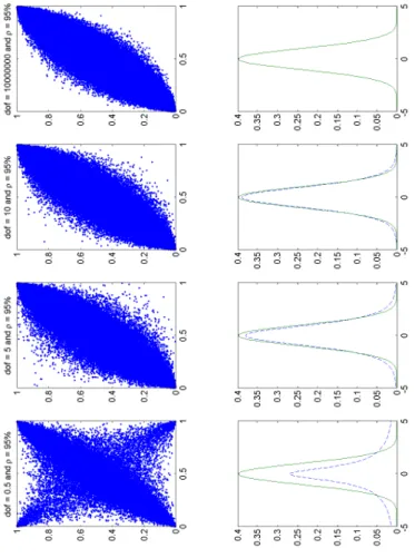
Figure 2.1: Shows varying 95% correlated random uniforms sampled from the Student-t copula with varying degrees of freedom. As the degrees of freedom tend to infinity, in the last graph its 10 000 000, the Student-t copula turns to the nor-mal copula, which is also confirmed by the corresponding pdfs of the graphs shown underneath. The dashed graph is that corresponding to the Student-t pdf, while the full line is a a standard normal pdf.

(37)

Chapter 3

Counterparty Credit Risk

Management

The traditional approach to counterparty credit risk has been the calculation of exposure profiles which would indicate how bad the losses would be if a counterparty were to default. This is usually done under the real-world probability measure, that is, there is extensive use of historic data in trying to understand future scenarios. This has, however, changed to pricing counterparty credit risk under the risk neutral measure and using existing credit derivatives to actively hedge the risk. This chapter explores various approaches to counterparty credit risk management.

3.1 A Model for the Economy

The economy is modelled using a probability space (Ω,F,(Ft)t≥0,P). The filtration (F_t)t≥0 models the flow of information of the whole economy, including defaults.

Defaults are characterized by default times which we denote by τi for a defaulting entityiandRi_tfor its recovery rate. An equivalent martingale measure ˜Pis assumed, under which the discounted price processes of all tradeable securities are martingales. The probability space has a right-continuous and complete sub-filtration (Gt)t≥0

representing all the observable market quantities excluding default events. Default events are contained in a right-continuous filtration generated by the default events, that is,

D_t=σ({τA≤u} ∨ {τB ≤u} ∨. . .∨ {τZ ≤u}:u≤t). (3.1) The relation between the filtrations is thus Gt⊆ Ft: =Gt∨ Dt[18]. The symbol ∨ should be interpreted to mean that Ft is the smallest σ-algebra containing Gt and D_t. The economy is further equipped with an instanteous spot rate rt, also known

(38)

3.2. COUNTERPARTY CREDIT RISK MITIGATION 27

as the short rate, such that the stochastic discount factor is given by, D(t, T) = exp − Z T t rsds . (3.2)

The discount bonds at t maturing T will be denoted by B(t, T). The existence of the equivalent martingale measure rules out any arbitrage opportunities.

3.2 Counterparty Credit Risk Mitigation

CCR mitigation techniques are to a large degree well supported by the ISDA master agreement. Under the ISDA master agreement, legally binding clauses exist, most of which were lobbied for by the ISDA itself to form part of legislation regulating the financial industry. The document also specifies procedures to be followed on occurrence of a default event involving one of the counterparties. The ISDA master agreement rigorously defines what constitutes a default event thus alleviating the ambiguity that often characterizes legal contracts. A default event is described as one of the following: bankruptcy, failure to make due payments on loans or bonds, repudiation or moratorium, cross-acceleration, obligation default, distressed structuring and credit event upon mergers.

Two mechanisms that aid in mitigating CCR that are also supported by the ISDA master agreement are netting and close-out netting. Netting allows for the offsetting of exposures between counterparties. Contracts that are netted should be under the same master agreement. The risk mitigation introduced by netting is obvious and illustrates the benefits associated with dealing with the same counterparties; however this benefit needs to be adequately managed as it might lead to poorly diversified portfolios of derivatives. Netting generally gives preference to derivatives dealers over other creditors of the same counterparty since the netting implies that they receive liquidation proceeds before other creditors do. Bliss and Kaufman [7], however, argue that the reason often given in legislative documents for allowing netting, that is, derivatives markets are more exposed to systemic risk, is not enough on its own to justify its existence. They note that there is no clear evidence of reduced systemic risk due to netting/close-out netting. The close-out clause allows one counterparty to unilaterally close out all positions at the same time under certain circumstances [7]. Duffie et al [29], point out that with two counterparties A and B, such that A always has a better credit rating than B, when netting across a swap portfolio, A seems to be at an advantage at the expense of B.

Netting on its own is only effective if there are to be a significant number of contracts entered into by both parties — this may be impractical for corporates not in the financial sector. This is due to the fact that corporates merely use the

(39)

3.2. COUNTERPARTY CREDIT RISK MITIGATION 28

contracts as hedging tools and may tend to hold the same positions in most of them, and they may also not hold a substantial number to make netting worthwhile. How-ever, corporates could in turn activate the credit support annex (CSA) on the ISDA master agreement as a means of mitigating CCR through the posting of collateral. The CSA defines the conditions under which collateral must be posted [3, 1]. The most important terms contained in the CSA from a modelling perspective include,

• Threshhold: The credit one party extends to the other counterparty [12,

41, 3]. It is that amount that is allowed to accumulate without the other counterparty having to post collateral, where it is used we will denote it by Ht. The counterparty is not required to pay off the threshhold, only what accumulates after taking into consideration theminimum transfer amount.

• Minimum Transfer Amounts : This is the minimum amount that is allowed

to accumulate beyond the thresh-hold before collateral is posted. It is intended to allow reasonable price movements before collateral is posted and where it is used we will denote it by Mt.

• Eligible Securities and Currencies : This is self-explanatory but it has

serious modelling consequences. Fujiiet al [42], investigate the use of different currencies because during the financial crisis, for example, it was expensive to use dollars as collateral. This was widely due to the fact that most parties were buying more dollars as a reserve currency.

A way to appreciate the effects of collateral is to imagine a deal in the presence of a CSA with Ht = Mt = 0 and the margin call frequency being continuous. In this scenario all the counterparty risk is eliminated. This is not very unrealistic as margin call frequency is usually daily. According to the ISDA about 30% of all OTC derivatives were collateralized in 2003 while at the end of 2009 about 78% of all OTC trades were collateralized. This in part is due to the financial crisis, but it is expected that this upward trend will continue. There are two approaches to collateral posting, unilateral and bidirectional. In unilateral posting only one party is required to post collateral (usually the party of much inferior credit quality), while in bidirectional posting both parties are required to post collateral (usually where the credit qualities of both parties are similar). Bidirectional posting is often facilitated by a third party called acentral clearing counterparty1. The existence of a central clearing counterparty and its effects are investigated by Duffie et al [32], where they conclude that the use of multiple clearing counterparties may reduce

1

This party is responsible for administering the process, that is, requesting, receiving and deposit-ing collateral to the correct account.

(40)

3.3. COUNTERPARTY CREDIT RISK METRICS 29

netting benefits especially with specialized clearing counterparties, who only clear a particular derivative contract. Advantages that a central clearing counterparty may bring include multilateral netting2.

The continued use of collateral has challenged traditional pricing theory that relies on the existence of a risk free rate that should be used to discount cash flows. The collateral posted, which is mainly in the form of cash in some of the developed currencies earns its own rate called the collateral rate,ct. The industry standard has now changed to discounting all cash flows using the overnight swap curve. Piterbarg [65] derives a Black-Scholes partial differential equation variant that all derivatives under collateral agreements should satisfy. He further prices some basic derivatives like forwards under the framework. Fujiiet al [39, 40, 41] constructs various curves for discounting cash flows that are collateralized and uncollateralized, with some in the presence of multiple currencies.

3.3 Counterparty Credit Risk Metrics

The management of counterparty risk has been practiced for years and risk desks use several metrics to gain insight into exposure to a counterparty. We only describe a few of these below while a full description is given by Gregory and Canabarro et al [47, 20]. In what follows we assume the total value of the portfolio to a particular counterparty at time t, denoted by Vt, is the sum of the individual instruments in the portfolio denoted byV_ti wherei= 1, . . . , N.

• Counterparty Exposure: This is the most basic measure. It is the

maxi-mum of zero and the market value of the portfolio attributed to the counter-party. It is the value that would be lost if the counterparty were to default with zero recovery, i.e.,

CE(t) = max{Vt,0}. (3.3)

Indeed, this is an extreme measure since it is virtually impossible that there would be zero recovery. The above equation assumes the presence of a netting agreement. If there is a partial netting agreement covering onlyKinstruments in place the equation becomes,

CE(t) = max ( _K X i=1 V_ti,0 ) + N X i=K+1 maxV_ti,0 . (3.4)

2_{Multilateral netting is when contracts are netted between a number of counterparties. It may}