University of Richmond
UR Scholarship Repository
Honors Theses Student Research
2017
The College Admissions Problem: Effects of
Income and Ability of Postsecondary Education
Outcomes
Martha Whamond
Follow this and additional works at:http://scholarship.richmond.edu/honors-theses Part of theEconomics Commons
This Thesis is brought to you for free and open access by the Student Research at UR Scholarship Repository. It has been accepted for inclusion in Honors Theses by an authorized administrator of UR Scholarship Repository. For more information, please contact
[email protected]. Recommended Citation
Whamond, Martha, "The College Admissions Problem: Effects of Income and Ability of Postsecondary Education Outcomes" (2017). Honors Theses. 1001.
The College Admissions Problem:
Effects of Income and Ability of Postsecondary Education Outcomes by Martha Whamond Honors Thesis Submitted to Department of Economics University of Richmond Richmond, VA April 29, 2017
Abstract
This paper examines the effects of students’ pre-college income on student outcomes and college admissions decisions. Under the assumption that colleges maximize utility by
maximizing student outcomes, a two-stage regression model for student outcomes is building using data from the Integrated Postsecondary Education Data System (IPEDS) and the 1997 National Youth Longitudinal Survey (NLSY97). The first stage estimates a model for college quality using the IPEDS dataset. The college quality estimates are then used as independent variables in the second stage. The second stage estimates student outcomes as a function of pre-college income, ability, pre-college quality, and demographic characteristics using the NLSY97 dataset. The results suggest that pre-college income has a positive and significant effect on post-college income but does not have a significant effect on post-college GPA. Conversely, the results suggest that student ability has a positive effect on college GPA but does not have a significant effect on post-college income. Assuming colleges consider post-college income potential as a factor in admissions decisions, the results indicate that a higher pre-college income would make a student more attractive to a college because the student is more likely to have a positive outcome.
1
1. Introduction
Higher-education has become an increasingly important topic of discussion and research as income inequality grows in the United States (Orentilcher, 2016). Many students choose to attend college, investing both time and money, with the assumption of higher lifetime earnings. For low-income students, the chance to attend college can mean breaking the poverty cycle (Sacks, 2007; Fischer, 2007), yet upwards of 80% of high-income students enroll in and complete college while the same is true for only 45% of low-income students (U.S. Bureau of Labor Statistics, National Center for Education Statistics, 2015). Undoubtedly, the high average annual tuition of $37,990 to attend a four-year college deters the low-income students (Digest of Education Statistics, 2015). Despite the availability financial aid has increased to $183.7 billion and the availability of loans has improved such that the aggregate student debt has surpassed credit card debt in the U.S. (McGrath, 2014). With the increased availability of student aid, there may be another reason fewer low-income students are attending college: who is admitted. Most college admissions policies are driven by the “effective marginal cost” of educating a student depending on ability and income (Epple, Romano, & Sieg, 2006).
This research examines how a student’s pre-college family income and ability affect college
admissions decisions.1 Under the assumption that colleges maximize utility by maximizing
student outcomes, a model is built to assess how income affects student outcomes controlling for ability, college quality and demographics. The model is a two-stage regression. The first stage estimates college quality based on college characteristics. The second stage estimates student outcomes as a function of college quality, pre-college family income, student ability and demographic characteristics. By using multiple measures of income, quality, and student
1
For the purposes of this paper, four-year institutions of higher education will be referred to as colleges which include undergraduate divisions of universities.
2 outcomes, the results are robust and inclusive of 60 regressions. The findings suggest the pre-college family income of a student positively impact a student’s post-graduation income but are not a significant factor in determining their college GPA. Conversely, the findings also suggest that student ability, measured by standardized test scores, are insignificant in predicting post-college income but are significant in predicting post-college GPA.
2. Literature Review
There is both breadth and depth in the existing literature on higher education and student outcomes. The literature spans a variety of disciplines and topics. The first section of this literature review will focus on the quality of colleges. The second section will focus on college attendance and student outcomes.
2.1 College Quality
Colleges are valued on the perception of quality and status (Kilgore, 2009), making the evaluation of college quality a complex task because perception is often far from reality. The phenomenon of ranking colleges became prominent in the late 1990s from a growing public demand for accountability and assessment of colleges and universities (Hossler, 2000). The value placed by prospective students and their families on published college rankings is concerning because rankings are not a consistent indicator of college quality. In fact, the majority of
variation in the prominent “Best College” rankings published by U.S. News and World Report
result from changes in how the rankings are calculated (Dichev, 2001). Only approximately 10% of the variation resulted from changes in the colleges (Dichev, 2001). The National Survey of Student Engagement (NSSE), generally considered a strong metric of university quality, has few
statistically significant correlations with US News Rankings (Pike, 2004). Although the rankings
3 be easily manipulated. The ability for manipulation encourages inefficient admissions policies. For example, urging below standard students to apply in order to inflate the applicant pool without increasing acceptances, or rejecting overqualified students to maintain a low admissions rate (Avery, Glickman, Hoxby, & Metrick, 2012).
College quality should be measured using resources like such as the NSSE. Pike (2004) finds that educational quality is increased by student engagement in activities that lead to learning. In addition to reputational measures such as rankings, colleges are frequently assessed on faculty scholarship and student experience (Brooks, 2005). While faculty research could be indicative of educational quality, it provides a major advantage to large colleges (Brooks, 2005). Brooks (2005) argues that student experiences, particularly program effectiveness which is often measured by graduation and completion rates, are the most indicative of college quality.
2.2 College Decisions and Outcomes
According to Gary Becker’s theory of human capital, the decision of attending college or immediately enter the labor is an investment decision (2008). The individual will attend college if the direct and opportunity cost of attending is outweighed by the enhanced wages they would earn with the additional education (Becker, 2008). In addition to intellectual ability, students consider the availability of financial resources to fund their education whether it is a bequest from their family, a grant from a college, or student loans.
Empirical evidence suggests that high-income, low-ability students are more likely to attend college that low-income, high-ability students (Kahlenberg, 2006). There is a variety of research studying exactly how availability of financial resources impacts the decision to attend college. Children born into a household with higher wealth are statistically more likely to attend college and graduate on time (Loke, 2013). However, children whose households accumulate
4 substantial wealth, even if the starting wealth at birth was low or zero, can have similar outcomes to the children born into wealthy households (Loke, 2013). College attendance is strongly linked with housing wealth because families, particularly those with a lower resource level, frequently finance their children’s post-secondary education with their housing wealth (Lovenheim, 2011). Increased housing wealth is linked not only with attending college but attending a higher quality college (Lovenheim & Reynolds, 2013). Epple, Romano and Sieg (2006) create a model such that colleges maximize utility by providing the highest quality educational experience to their students. This model posits that the quality of the education experience is derived from
instructional expenditures and the quality of a student’s peers, the student body (Epple, Romano, & Sieg, 2006). Their findings suggest that admissions policies are largely driven by applicants’ ability and income because there are varying effective marginal costs of education students based on their abilities and incomes (Epple, Romano, & Sieg, 2006).
3. Theoretical Framework
Colleges do not maximize utility by maximizing profit because the majority of four-year colleges in the United States are either public or private not-for-profit. Epple, Romani & Sieg (2006) construct a model in which colleges maximize the quality of the educational experience for their students. With this premise, a college maximizes utility by fulfilling its mission. Most baccalaureate college mission statements include some variation of student success (Taylor & Morphew, 2010). Consequently, colleges maximize utility by maximizing student success. Student success is measured by quantifying student outcomes. The utility maximizing college should admit the student who is most likely to be successful.
The purpose of this research is to identify how pre-college family income affects college admission decisions. If pre-college family income is a significant factor in determining student
5 outcomes, colleges will admit a higher-income student over a lower-income student with equal qualifications. The primary model estimates student outcomes as a function of pre-college family income, student ability, quality of the college attended, and demographic characteristics.
Multiple measurements of each factor are used to test robustness of the results.
The primary dataset for this research, the NLSY97, provides information on pre-college family income, student intellectual ability, characteristics of the college attended, and
demographic characteristics. The NLSY97 does not include quality of the college attended. From a secondary dataset on colleges, the quality of a college is modeled using the same characteristics identified in the primary dataset. The college quality estimation is then applied to the primary dataset and calculated for each individual based on the reported characteristics of his or her college.
4. Data
The primary dataset from the 1997 National Youth Longitudinal Survey (NLSY97). The NLSY97 dataset contains information that measures student outcomes, student ability, pre-college family income, demographic characteristics, and pre-college characteristics. The secondary dataset is from the Integrated Postsecondary Data System (IPEDS). The IPEDS dataset contains information about institutions of higher education in the United States, including measures used to estimate quality and characteristics of the colleges.
4.1 Integrated Postsecondary Data System Dataset
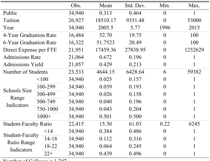
The IPEDS contains of information for 7,481 institutions of higher education. The dataset used in the analysis contains information for 1,747 colleges. The criteria for colleges in the sample are: (1) public or private not-for-profit sectors; (2) degree-granting; (3) primarily baccalaureate of above; and (4) full-time undergraduates. Descriptive statistics of the IPEDS
6 dataset appear in Table 1. Specific definitions of variables and additional definitions are in Table 2. The IPEDS data are from 1996-2015 to coincide with the NLSY97 dataset. Colleges report information annually. Some measurements such as six-year graduation rate, have not been mandated to report since 1996, accounting for the discrepancy in observation number. In
additional to actual number of students and actual student-faculty ratio, binary variables indicate ranges of number of students and student-faculty ratio in which the colleges belong. The
NLSY97 does not include actual number of students or actual student-faculty ratio. Instead, the NLSY97 includes ranges of number of students and ranges of student-faculty ratio the youth selects for their college. The binary variable indicators created in the IPEDS dataset are consistent with the ranges in the NLSY97 dataset and are used in the empirical models.
Measurements of college quality are still debated. To ensure a robust analysis, five measurements of college quality are estimated to be used in the primary model: (1) four-year graduation rate; (2) six-year graduation rate; (3) direct expenses per FTE; (4) admissions rate; and (5) admissions yield. Brooks (2005) argues that four and six-year graduation rates are the most indicative measures of program effectiveness and college quality so both rates were used. In addition to graduation rates, direct expense per student is included to assess the financial investment colleges make in students. Higher investment should lead to a higher quality
education. Admissions rate and yield are two key metrics included in most ranking calculations, such as U.S. News & World Report (Morse, Brooks, & Mason, 2016). Although the significance of published rankings is highly debated, many prospective students and parents still use these rankings to help evaluate potential colleges.
7
4.2 National Youth Longitudinal Survey, 1997 Cohort
The NLSY97 is a longitudinal survey of approximately 9,000 young men and women in the United States born between 1980-84. The youths were between the ages 12-16 at the time of the first interview and reached age 18 between 1998 and 2002. The youths were interviewed for one-hour, annually starting with Round 1 in 1997. Parents were also interviewed during Rounds 1-5. As of January 2017, data from Rounds 1-16 are publicly available. The survey provides information on education, employment, family life, income, health, attitudes, and criminal activity. Of the original 8,984 youth cohort, 4,060 attended a four-year college at some point. Only 814 of those 4,060 youths provided enough information to be included in this analysis, creating the possibility of selection bias. Table 3 provides descriptive statistics and specific variable definitions are presented in Table 4.
Post-college income and College GPA are the two metrics used to estimate student
outcomes. Some students attend college because they believe it will provide them an opportunity to earn a higher wage post-college (Cilesiz & Drotos, 2016). Other students attend college to pursue further education or to have the necessary credentials to earn a position in public service. For example, a student would be considered highly successful in college if he or she earned a high enough GPA to attend medical school. However, the student would be in graduate school and residency for over seven years after graduating college, resulting in a lower post-college income that is not indicative of the successful outcome. Household income and poverty ratio are used to measure pre-college family income. The SAT and converted ACT scores are used to estimate a student’s intellectual ability. 2
2
Most colleges in the United States require submission of SAT or ACT scores to be included in applications for admission. ACT scores were converted to SAT scores because the SAT is more common.
8 The last group of variables included in the NLSY97 dataset is college characteristics. The IPEDS dataset includes multiple observations across years which provide more information in comparison to aggregating by college. The “Year” variable in the IPEDS dataset corresponds with the “First Year of College” variable in the NLSY97 dataset. It is important to note that in contrast to the IPEDS dataset, where only 30% of the colleges were public, approximately 83.8% of students in the NLSY97 dataset attended a public college. However, the IPEDS data set counts number of colleges whereas the NLSY97 dataset counts number of students. Public colleges tend to be larger when analyzing the number of students at each college. In the IPEDS dataset, where exact number of students is provided, public and number of students have a correlation coefficient of 0.61 (see Table 5).
5. Empirical Model
This analysis uses a two-stage regression model. The first stage estimates the quality of a college using key characteristics. The first-stage estimation is performed using the IPEDS dataset for 1,747 colleges. The coefficients of the college characteristic variables are used in the second stage to weight the characteristics of the college the youth attended. Since data on the specific college the student attended is unavailable, using weighted college characteristics to estimate quality links the primary and secondary datasets. This step provides a measure of college quality to be included in the model for student outcomes.
5.1 College Quality
The first-stage regression estimates college quality, 𝑞𝑗. The five measures of college quality are four- and six-year graduation rates, direct expenses per FTE and admissions rate and yield (see section 5.1). The empirical model for quality of a college j, is specified in Equation 1:
9 (1) 𝑞𝑗 = 𝛾1(𝑟𝑎𝑡𝑖𝑜)𝑗+𝛾2(𝑠𝑡𝑢𝑑𝑒𝑛𝑡𝑠)𝑗+𝛾3(𝑡𝑢𝑖𝑡𝑖𝑜𝑛)𝑗+𝛾4ln(𝑡𝑢𝑖𝑡𝑖𝑜𝑛)𝑗+𝛾5(𝑝𝑢𝑏𝑙𝑖𝑐)𝑗+ 𝛾6(𝑦𝑒𝑎𝑟)𝑗+𝛼1+𝜀𝑗 where 𝑞𝑗 = quality 𝑟𝑎𝑡𝑖𝑜 = student-faculty ratio 𝑠𝑡𝑢𝑑𝑒𝑛𝑡𝑠 = number of students 𝑡𝑢𝑖𝑡𝑖𝑜𝑛 = tuition 𝑝𝑢𝑏𝑙𝑖𝑐 = public sector 𝑦𝑒𝑎𝑟 = year 𝛼1 = constant 𝛾1- 𝛾6 = estimated coefficients
Low student-faculty ratios are considered desirable characteristics of a college because students have more opportunity to interact with faculty members. As student-faculty ratio decreases, quality is expected to increase. Similarly, small colleges are often equated with high quality because of the increased faculty interaction. However, large colleges can be desirable because they are more likely to have robust research programs. Strong research programs are more likely to have access to resources such as grants for which small colleges do not have economies of scale (Brooks, 2005). The expected effect of college size on college quality is ambiguous because small and large colleges can be desirable. While high tuition is not desirable by prospective students and their families, some are willing to pay higher tuition if the college is higher quality. By this logic, as tuition increases quality should increase. However, there are likely diminishing marginal returns increased tuition, captured by the logarithmic term. Lastly, public colleges have earned the reputation of being lower quality due to large class sizes and preferential admissions of in-state or in-district students. Conversely, large public colleges often have access to resources small private colleges may not be able to finance, making the effect of sector on college quality ambiguous.
10
5.2 Student Outcomes
The second stage of the regression models student outcomes as a function of pre-college income, student ability, college quality, and control variables. The initial model for the outcome of a student i attending a college j, is specified in Equation 2:
(2) (𝑂𝑢𝑡𝑐𝑜𝑚𝑒)𝑖,𝑗 =𝛽1(𝑤𝑒𝑎𝑙𝑡ℎ)𝑖+𝛽2(𝑎𝑏𝑖𝑙𝑖𝑡𝑦)𝑖+𝛽3 𝛾1(𝑟𝑎𝑡𝑖𝑜)𝑗+𝛾2(𝑠𝑡𝑢𝑑𝑒𝑛𝑡𝑠)𝑗 + 𝛾3(𝑡𝑢𝑖𝑡𝑖𝑜𝑛)𝑗+𝛾4ln(𝑡𝑢𝑖𝑡𝑖𝑜𝑛)𝑗+𝛾5(𝑝𝑢𝑏𝑙𝑖𝑐)𝑗+𝛾6(𝑦𝑒𝑎𝑟)𝑗+𝛼1 +𝛽4(ℎℎ𝑠𝑖𝑧𝑒)𝑖+ 𝛽5(𝑝𝑎𝑟𝑒𝑛𝑡)𝑖+𝛽6(𝑠𝑒𝑥)𝑖+𝛽7(𝑤ℎ𝑖𝑡𝑒)𝑖+𝛼2+𝜀𝑖,𝑗
and the simplified model is presented in Equation 3:
(3) (𝑂𝑢𝑡𝑐𝑜𝑚𝑒)𝑖,𝑗 = 𝛽1(𝑤𝑒𝑎𝑙𝑡ℎ)𝑖+𝛽2(𝑎𝑏𝑖𝑙𝑖𝑡𝑦)𝑖+𝛽3𝑞𝑗+𝛽4(ℎℎ𝑠𝑖𝑧𝑒)𝑖+𝛽5(𝑝𝑎𝑟𝑒𝑛𝑡)𝑖+𝛽6(𝑠𝑒𝑥)𝑖+ 𝛽7(𝑤ℎ𝑖𝑡𝑒)𝑖+𝛼2+𝜀𝑖,𝑗 where 𝑂𝑢𝑡𝑐𝑜𝑚𝑒 = student outcome 𝑤𝑒𝑎𝑙𝑡ℎ = family income 𝑎𝑏𝑖𝑙𝑖𝑡𝑦 = student ability
𝑞𝑗 = estimated college quality
ℎℎ𝑠𝑖𝑧𝑒 = household size 𝑝𝑎𝑟𝑒𝑛𝑡 = parent education 𝑠𝑒𝑥 = sex 𝑤ℎ𝑖𝑡𝑒 = race/ethnicity 𝛼2 = constant 𝛽1- 𝛽7 = estimated coefficients
The purpose of this research is to determine how family income affects a student’s outcome. Given that students with higher family income are more likely to attend college, less likely to work during college, and more likely to have parents that attended college (Loke, 2013), family income should have a positive effect on student outcomes. Similarly, a higher ability student earning a higher standardized test score is more likely to have a better outcome. Higher quality
11 colleges should also lead to improved student outcomes as the mission of most colleges to
maximize student success (Taylor & Morphew, 2010).
Household size, parent education, sec and race/ethnicity are all demographic control variables, however, literature suggests that all four effect the decision to attend college (Cohn, Cohn, Balch, & Bradley, 2004; Cilesiz & Drotos, 2016). As household size decreases, the youth is likely to have more financial resources and parent/guardian attention. However, if the youth lives with just one parent/guardian he or she may need to contribute more to the household, decreasing time spend on education. In aggregate, household size is expected to have a negative effect on outcomes. One of the main reasons students attend and complete college is whether or not there are parental expectations to attend (Lovenheim, 2011). The expectation to attend college is most likely in a home where parents went to college, causing parent education to create a positive effect on student outcomes. Females tend to have higher grades in comparison to males (Routon & Walker, 2014) although males tend to have higher incomes compared to females (Blau & Kahn, 2007), creating an ambiguous effect because post-college income is also effected by grades in college. Lastly, more white students attend and complete college.
Approximately 85% of non-white, non-Asian minorities attend predominantly white institutions (PWI) where minority students have well-documented challenges with social and academic success (Fischer, 2007). White students are expected to have better post-college outcomes.
6. Results
To ensure robust results, a total of five models for college quality, using the five different metrics, and twenty models for student outcomes, using all combinations of metrics discussed (see section 4.2) are estimated.
12
6.1 School Quality
The first-stage regressions, using all five metrics for college quality, were estimated using a robust OLS regression. The results of these models are presented in Table 10. While the quality of public versus private not-for-profit colleges is debated and the predicted effect was
ambiguous, the results in all five models public colleges are higher quality. The significance of both tuition and the natural logarithm of tuition suggest a non-linear relationship consistent with the assumption of diminishing marginal returns. The positive relationship with the linear term for tuition is consistent across all models3 and suggests that tuition positively affects college quality. School size is particularly complex to interpret because over 50% of the colleges in the dataset have more than 1,000 students. While there are significant binary variables, there is not a uniform trend across models.
The models that include Direct expense per FTE, Admissions Rate, and Admissions Yield all suggest a negative and decreasing coefficient as college size increases. However, if this were a standard trend, the coefficients for admissions rate should be inversed. The analysis is
conducted using only colleges over 1,000 students and, therefore, excluding the college size variable to test for robustness of the results (see Section 7.1). As predicted from the literature review, quality generally increases as student-faculty ratio decreases. The highest range of student-faculty ratio was greater than 22. This range was excluded for colinearity. Positive coefficients on all other ranges indicate increasing quality as student to faculty ratio decreases. The trend of increasing quality as faculty ratio decreases is strongest among student-faculty ratios less than 14. The coefficient associated with the binary variables for student-student-faculty ratio less than 14 is positive and significant for all measurements except admissions yield. Lastly,
3
Recall that quality increases as admissions rate decreases, explaining the variation in the sign of the coefficients for admissions rate.
13 it is important to note that the R-Square value for four- and six-year graduation rates and
admission yield are all more than double the R-Square values for Direct expense per FTE and admissions rate.
6.2 Student Outcomes
As mentioned above, there are twenty baseline models for student outcomes that include combinations of dependent variables and independent variables to ensure robust results. The results are separated into five tables, each containing four models, and a different estimated quality measure in each table. For clarity while comparing the models, Table 11 shows which variables are included and how the models are organized. The regression results for each model are included in Tables 12 – 16.
The first set of models (see Table 12) include four-year graduation rate as the estimator for college quality. The coefficient for household size is only significant in Model 1. As expected, household size is not significant in Model 2 or Model 4 because Poverty Ratio already corrects for household size. The negative and significant coefficient suggests that for a decrease in household size by one person, the student will earn an extra $3,102 annually after college. The negative and significant coefficient suggests that a smaller household is linked with higher earning students after college.
Interestingly, parent education is negative and significant in Models 1 and 2 and
insignificant in Models 3 and 4. Models 1 and 2 actually suggest that a student earns $889.70 and $933.20 less annual after college for each additional grade of education their parent has earned. Although this initially seems counterintuitive, higher education levels are generally correlated with higher incomes. If the child of a higher educated parent grows up with more financial
14 stability, the child may be more willing to enter a lower income profession that they derive a higher level of enjoyment from knowing they have a financial safety net.
Race, measured by the White indicator variable, is positive and significant for Models 3 and 4 but insignificant in Models 1 and 2. Given the smaller share of non-white students in higher education and the lower average socioeconomic status, it is expected that white students have higher GPAs, as shown in Models 3 and 4. There is an abundance of research on how race affects college outcomes, especially since race is often correlated with socioeconomic status. Fischer (2007) suggests that black and Hispanic students are less successful academically because they are less likely to have the same support networks at home, linked with
socioeconomic status, and on campus, especially for minority students at PWIs. Conversely, a qualitative research study of high poverty students, an above average share of whom were Hispanic and/or black, reported one of the main reasons for attending college to be future economic security (Cilesiz & Drotos, 2016). The trend suggests that white students may have higher College GPAs but non-white minority students are equally as focused on earning a high post-college income.
Consistent with macroeconomic trends, males have a significantly higher post-college income than females in both Models 1 and 2. The model does not correct for occupation which is a key factor in determining income, especially since males and females tend to choose different occupations. Additionally, a gender based pay-gap is widely cited and while its exact value is debated, the existence of the pay-gap is generally accepted (Blau & Kahn, 2007). Research of students that were first-year undergraduates in 2000 and 2001, approximately when the youths in the NLSY97 cohort were turning 18, the start of typical college age, suggest that men are less
15 likely to earn and maintain a higher GPA than females (Cohn, Cohn, Balch, & Bradley, 2004), supporting the findings in Models 3 and 4.
The SAT score binary variables complicate the understanding of the results. In Model 1, none of the dummy variables for SAT Score were significant. In Model 2, only the lowest score range was significant. However, the negative and significant coefficient associated with the lowest score range supports the hypothesis that higher SAT scores lead to better student outcomes. Similarly, in Models 3 and 4, negative coefficients for the 801-1000 range are significant, supporting the same theory. Additionally, the highest SAT Score range, 1401-1600 are positive and highly significant for estimating college GPA. To test the joint significance of the SAT Score indicator variables, a series of F-tests were performed which will be discussed in the next section.
The estimated measure of college quality, four-year graduation rate, is positive and significant across all four models. Although the coefficients are significant the magnitude
suggests only a minor impact. For Models 1 and 2, a one percentage point increase in graduation rate only suggests an increase in post-college income of approximately $110. For Models 3 and 4, a one percentage point increase in graduation rate increases college GPA by approximately 0.9 on a 400-point scale, which equates to an increase of 0.01 on the traditional 4.0 scale.
Household income in high school and poverty ratio are both highly significant and positive indicators of post-college income. However, household income and poverty ratio do not have a significant effect on college GPA as originally hypothesized. Household income in high school and post-college income were had a correlation coefficient of 0.4295 (see Table 7). Household income in high school and college GPA only had a correlation coefficient of 0.0836.
16 The trends in the results for Models 1-4 discussed above for household size, parent
education, race/ethnicity, sex, household income in high school, and poverty ratio are constant across Models 5-20 when the quality estimator is changed. Six-year graduation rate was positive and significant, with similar values in magnitude to four-year graduation rate, across Models 5-8 (see Table 13). Direct expense per FTE, presented in Table 14, was not a significant in
estimating post-college income in Models 9 and 10. Although Direct Expense per FTE was significant in Models 11 and 12 in predicting College GPA, the magnitude suggests that a $10,000 increase in Direct Expenses only improves college GPA by 0.06 on the traditional 4.0 scale. Admissions Rate, included in Table 15, was negative and significant across Models 13-16 as expected because quality increases as admissions rate decreases. Admissions Yield, included in Table 16, was insignificant in estimating post-college income in Models 17 and 18. However, Admissions yield was positive and highly significant in predicting College GPA with a relative large magnitude of an additional 0.40 increase in GPA on the traditional 4.00 scale for every one percentage point increase in Admissions Yield.
6.3 Joint Significance of Student Ability
Student ability, measured by SAT Score, is significant in some ranges in some models but there is not a consistent trend across models like the other variables. Since the data structure required the model to be specified as five dummy variables, an F-Test for joint significance was performed for Models 1-20 by generating a restricted and unrestricted model and calculating the F-Statistic (see Appendix, Eq. A-1). The unrestricted model includes the SAT Score dummy variables and the restricted model excludes the SAT Score dummy variables (see Appendix, Eq. A-2 to A-4)
17 The results of the F-Tests are included in Table 17. The F-Statistic is significant at the 1% or 5% level for all models that include College GPA as the independent variable. The F-Statistics for these models are close in magnitude ranging from 3.25 to 3.42. Between groups of models
where the only change is the measurement of income,4 the F-Statistic is only different by 0.01 or
less. However, the F-Statistics in the models where post-college income is used at the
independent variable are all insignificant even at the 10% level. The consistency of these results suggests pre-college ability, measured by SAT Score, is significant in predicting College GPA but is insignificant in predicting post-college income.
7. Robustness
Although five models for college quality and twenty models for student outcomes were analyzed, two more tests for robustness were analyzed. The first robustness check is the same procedure excluding colleges with enrollment less than 1,000 students. The second robustness check includes college GPA as an independent variable while maintaining post-college income as the dependent variable.
7.1 School Size
Over 50% of the colleges analyzed in the IPEDS data set had a student body of over 1,000. Recently, there have been news and media publications discussing the challenges facing small colleges with fewer than 1,000 students due to inefficiencies and a declining enrollment
(Selingo, 2016). The inefficiencies and declining enrollment suggest decreasing quality of these small colleges. None of the top 310 National Universities and only 27 of the top 239 Liberal Arts Colleges ranked by US News & World Report have fewer than 1,000 students (Best Colleges, 2016). To ensure that the trend is not affecting the results, the school quality estimation is
18 performed only using colleges with greater than 1,000 students and eliminating college size as an independent variable in the first-stage regression analysis.
7.1.1 College Quality
The same two-stage regression model is used in the robustness test as the method for the baseline results. All five metrics of college quality are estimated on the limited subset of colleges with over 1,000 students and the independent variable for college size is eliminated. The
empirical model for the quality of a college j, is specified in Equation 4:
(4) 𝑞𝑗 = 𝛾1𝑟𝑗+𝛾2𝑡𝑗+𝛾3ln𝑡𝑗+𝛾4𝑝𝑗+𝛾5𝑚𝑗+𝛼1+𝜀𝑗, 𝑖𝑓 𝑛𝑗 >1000 where 𝑞𝑗 = quality 𝑟𝑗 = student-faculty ratio 𝑡𝑗 = tuition 𝑝𝑗 = sector 𝑚𝑗 = year 𝛼1 = constant 𝛾!- 𝛾! = estimated coefficients 𝑛𝑗 = number of students
The results of the adjusted analysis are included in Table 18. Although there is some variation in the magnitudes associated with each, the trends of direction and significance of the estimated coefficients remain the same for public, tuition, natural logarithm of tuition, and year. The trend of lower ranges of student-faculty ratio contributing to higher quality is consistent and there are more significant coefficients associated with the binary variables in the adjusted
analysis. The R-Square increases for Models F, G, and H in comparison to Models A, B, and C, respectively (see Table 10). The R-Square for Model J is only improved by 0.0006 compared to Model D. However, the R-Square decreases from 0.4808 in Model E to 0.1516 in Model K, suggesting that admission yield is a better estimator of quality for the subset that includes
19 colleges with fewer than 1,000 students. Despite the variation in R-Squares, the general trends of the results are consistent with the baseline analysis.
7.1.2 Student Outcomes
The adjusted coefficient estimates for college characteristics are used to estimate college quality for colleges with over 1,000 students in the NLSY97 dataset. Similar to the empirical model for college quality, the empirical model for student i attending a college j, before simplification, is specified in Equation 5:
(5) 𝐺𝑖,𝑗 =𝛽1𝑤𝑖+𝛽2𝑎𝑖+𝛽3 𝛾1𝑟𝑗+𝛾2𝑡𝑗+𝛾3ln𝑡𝑗+𝛾4𝑝𝑗+𝛾5𝑚𝑗+𝛼1 +𝛽4ℎ𝑖+
𝛽5𝑑𝑖+𝛽6𝑠𝑖+𝛽7𝑘𝑖+𝛼2+𝜀𝑖,𝑗, 𝑖𝑓𝑛𝑗 > 1000 and the simplified form of the model is specified in Equation 6:
(6) 𝐺𝑖,𝑗 =𝛽1𝑤𝑖+𝛽2𝑎𝑖+𝛽3𝑞𝑗+𝛽4ℎ𝑖+𝛽5𝑑𝑖+𝛽6𝑠𝑖+𝛽7𝑘𝑖+𝛼2+𝜀𝑖,𝑗, 𝑖𝑓 𝑛𝑗 > 1000 where 𝐺𝑖,𝑗 = student outcome 𝑤𝑖 = family income 𝑎𝑖 = student ability
𝑞𝑗 = estimated college quality
ℎ𝑖 = household size 𝑑𝑖 = parent education 𝑠𝑖 = sex 𝑘𝑖 = race/ethnicity 𝛼2 = constant 𝛽1- 𝛽7 = estimated coefficients 𝑛𝑗 = number of students
The adjusted models are included in Tables 19-23 and correspond with the models in Tables 12-16 such that Model 1A corresponds with Model 1. Model 1A includes the adjusted estimate of four-year graduation rate and Model 1 includes the baseline estimate of four-year graduation rate. Otherwise, Model 1A and Model 1 are identical. Before discussing specific trends between the adjusted and baseline models, it is important to note restricting the dataset to
20 colleges with 1,000 students or more decreased the number of observations in all models by over 200. Models 1A – 20A have the same trends regarding significance and direction of coefficients for Household size, Parent Education, Race/Ethnicity, Sex, Household Income, and Poverty ratio compared to Models 1 – 20, respectively. The adjusted results for the control variables and family income, measured as household income or poverty ratio are consistent with the baseline results, indicating robust results.
The adjusted results differ for some estimations of quality. In Table 19, the coefficient for four-year graduation rate is insignificant in Models 1A and 2A. Four-year graduation rate was positive and significant at the 10% level in Models 1 and 2 (see Table 12). The magnitude of the coefficients in Models 1 and 2 are relatively small suggesting that a weak estimator with minimal impact. However, four-year graduation rate was significant at the 1% level for Models 3 and 4 and remained significant at the same level for Models 3A and 4A. Additionally, the magnitude of these coefficients more than doubled suggesting that the adjusted four-year graduation rate is stronger estimator for College GPA but a weaker estimator for Post-college income. Six-year graduation rate was significant at the 5% level in Models 5 and 6 and at the 1% level in Models 7 and 8 (see Table 19). In the corresponding Models 5A-8A in Table 20, six-year graduation rate is insignificant in all four models. The result is unexpected since four- and six-year graduation rates are highly correlated. However, it is possible that higher quality colleges over 1,000 students have very few students graduate in six years so the variation would be too small in the adjusted subset to see significant impact.
The coefficients of the adjusted estimation of Direct Expense per FTE in Table 21 for Models 9A-12A are identical in direction and level of significance and similar in magnitude to the corresponding coefficients in Models 9-12 (see Table 14). Models 13A and 14A which
21 include Admissions Rate as the quality estimator include an insignificant coefficient for
admission rate. Similar to four-year graduation rate, admissions rate was only significant at the 10% level in Models 13 and 14 so the insignificance is reasonable. Admissions rate remained a significant factor at the 1% level in Models 15A and 16A. The same trend observed with admissions rate is consistent with the observed with admissions yield when comparing Models 17 – 20 and Models 17A – 20A (see Tables 16, 23). While there is some variation in the significance of quality estimators between the adjusted models and the baseline models for student outcomes, the overall trends held constant with the adjusted subset of colleges.
7.2 College GPA as an Independent Variable
The next test for robust is analyzing college GPA as an independent variable that contributes to Post-College income. Since post-college income and college GPA are used as alternate measures of outcomes, there is no test of how the variables are related besides their correlation coefficient which was 0.13 (see Table 7). For this test of robustness, the baseline results for college quality (see Table 4) are used and there is no change to the first-stage regression. Ten additional models were created using the following adjusted empirical model:
(1) 𝐺𝑖,𝑗 = 𝛽1𝑤𝑖+𝛽2𝑎𝑖+𝛽3𝑞𝑗+𝛽4ℎ𝑖+𝛽5𝑑𝑖+𝛽6𝑠𝑖+𝛽7𝑔𝑖+𝛽7𝑘𝑖+𝛽8𝑣𝑖+𝛼2+𝜀𝑖,𝑗
where
𝐺𝑖,𝑗 = post-college income
𝑤𝑖 = family income
𝑎𝑖 = student ability
𝑞𝑗 = estimated college quality
ℎ𝑖 = household size 𝑑𝑖 = parent education 𝑠𝑖 = sex 𝑘𝑖 = race/ethnicity 𝑣𝑖 college GPA 𝛼2 = constant 𝛽!- 𝛽! = estimated coefficients
22 The additional Models are located in Tables 24 – 26 and titled to correspond with the baseline models that included post-college income as the dependent variable. For example, Models 1B and 2B correspond with Models 1 and 2 (see Table 12) with the only difference being the inclusion of four-year graduation rate.5
College GPA is a consistent predictor of post-college income in all ten models (Tables 24-26). The economic significance of the coefficients implies that, for example in Model 1B, each additional 0.01 earned in GPA contributed to a $25.56 increase in annual income after college. While this may initially seem insignificant in magnitude, it suggests that an increase in GPA from 2.70 to 3.70 would earn an extra $2,556 annually after college.
Similar to the trends in the baseline model, household size is significant when family income is measured as Household income (Models 1B, 5B, 9B, 13B, and 17B) but is
insignificant when poverty ratio is used (Models 2B, 6B, 10B, 14B, 18B). This is expected because poverty ratio accounts for household size. Parent education has no significant coefficient in any of the models. Similar to the trend in the baseline results, Race/Ethnicity, measured by the binary variable white, does not have a significant coefficient for estimating post-college income. Again, consistent with the baseline model, the coefficient for male is consistently highly
significant and positive.
Both measures of family income, Household Income and Poverty Ratio, are highly significant and positive across all ten models. The positive sign and significance suggests that even when controlling for College GPA as an independent variable, pre-college income is still a key determinant in post-college income. Four- and six- year graduation rate are positive and significant at the 5% level in Models 1B-2B and 5B-6B. Direct Expenses per FTE is insignificant
5 Since only ten of the original twenty baseline models included post-college income as the dependent variable some of the adjusted models (indicated with B) are nonconsecutive in numbering.
23 in both Model 9B and Model 10B. Admissions Rate is significant at the 10% level in Models 13B and 14B. Admissions yield is insignificant in Models 17B and 18B. The trend of strong significant coefficients for both graduation rates suggests that graduation rates are the strongest indicator of college quality when College GPA is used as an independent variable. This is consistent with the initial baseline college quality results as the Models for four- and six-year graduation rates had the highest R-Square value of any of the five models.
8. Conclusion
The primary research purpose was to examine how pre-college family income affects college admissions decisions. The framework for the model works under the assumption that colleges maximize utility by maximizing student outcomes. Colleges, therefore, will accept students with the highest potential for success. The results suggest different conclusions depending on how student outcomes are measured. Pre-college income, estimated by family income and poverty ratio, does have a positive and significant effect on post-college income. Post-college income is also dependent upon the quality of the college, parent education, and sex. Interestingly, ability, measured by standardized test score, was not a significant factor in post-college income when controlling for income and post-college quality. When measuring student outcomes by college GPA, ability, quality of the school, sex, race were all significant factors but college income was an insignificant factor. The results imply that in addition to ability, pre-college family income may also be a factor because higher-income students are have a higher post-college earning potential.
Demographic control variables were included to capture any other trends. Consistently across all models, males had significantly higher post-college incomes and statistically
24 higher incomes after graduation. However, the models do not account for occupation after
graduation. Direction for further research includes testing the models with information on occupation or field of study. While white students had significantly higher college GPAs than non-white students, there was no statistically significant difference between post-college income for white and non-white students. Anecdotal evidence suggests that earning a higher income after graduation may be more important to non-white students because college represents a chance to break the poverty cycle. Another direction for further research is assessing with a larger sample set the outcomes of non-white students based on income to better understand if the trends are more closely related to race or socioeconomic status.
25
9. References
Avery, C. N., Glickman, M. E., Hoxby, C. M., & Metrick, A. (2012, December 13). A Revealed
Preference Ranking of U.S. Colleges and Univeristies. Quarterly Journal of Economics,
281(1), 425-467.
Becker, G. (2008). Human Capital. Retrieved from Library of Economics and Liberty: The
Concise Encyclopedia of Economics.
Best Colleges. (2016). Retrieved from US News & world Report.
Blau, F. D., & Kahn, L. M. (2007, June 29). The Gender Pay Gap. (M. Cragg, J. Stiglitz, & J. Zwiebel, Eds.) The Economists' Voice, 4(4), 5-11.
Brooks, R. (2005, Fall). Measuring University Quality. THe Review of Higher Education, 29(1),
1-21.
Bureau of Labor Statistics, U.S. Department of Labor. (1997-2013). National Longitudinal
Survey of Youth 1997 cohort. Columbus, OH: 2015: The Ohio State University.
Cilesiz, S., & Drotos, S. M. (2016). High-Poverty Urban High School Students' Plans for Higher
Education: Weaving Their Own Safety Nets. Urban Education, 51(1), 3-31.
Cohn, E., Cohn, S., Balch, D. C., & Bradley, J. (2004, December). Determinants of
undergraduate GPAs: SAT scores, high-school GPA and high-school rank. Economics of
Education Review, 23(6), 577-586.
Dichev, I. (2001, June). News or Noise? Estimating the Noise in the U.S. News University
Rankings. Research in Higher Education, 42(3), 237-266.
Education in the U.S. (2017, January 3). Retrieved from USA.gov.
Epple, D., Romano, R., & Sieg, H. (2006, July). Admission, Tuition, and Financial Aid Policies
26 Fischer, M. J. (2007, Mar. - Apr.). Settling into Campus Life: Difference by Race/Ethnicity in
College Involvement and Outcomes. The Journal of Higher Education, 28(2), 125-161.
Hossler, D. (2000). The Problem with College Rankings. About campus, 5(1), 20-24.
Kahlenberg, R. D. (2006, March). Cost Remains a Key Obstacle to College Access. The
Chronicle of Higher Education, 52(27), p. B. 51.
Kilgore, L. (2009, Summer). Merit and Competition in Selective College Admissions. The
Review of Higher Education, 32(4), 469-488.
Loke, V. (2013, April 1). Parental Asset Accumulation Trajectories and Children's College
Outcomes. Economics of Education Review, 33, 124-133.
Lovenheim, M. F. (2011). The Effect of Liquid Housing Wealth on College Enrollment. Journal
of Labor Economics, 29(4), 741-771.
Lovenheim, M. F., & Reynolds, C. L. (2013, Winter). The Effect of Housing Wealth on College
Choice: Evidence from the Housing Boom. Journal of Human Resources, 48(1), 1-35.
McGrath, M. (2014, December 29). Student Debt as an Asset Class: A $1 Trillion Opportunity? Forbes.
Morse, R., Brooks, E., & Mason, M. (2016, September 12). U.S. News & World Report. Retrieved from How U.S. News calculated the 2017 best college rankings.
National Center for Education Statistics. (1980-2016). Integrated Postsecondary Education Data
System. Institute of Education Sciences, U.S. Department of Education, Washington, D.C.
Orentilcher, D. (2016, September 22). Economic inequality and college admissions policies. Cornell Journal of Law and Public Policy, 26(1), 101-123.
27 Pike, G. R. (2004, March). Measuring Quality: A Comparison of "U.S. News" Rankings and
NSSE Benchmarks. Research in Higher Education, 45(2), 193-208.
Routon, P. W., & Walker, J. K. (2014). The impact of Greek organization membership on
collegiate outcomes: Evidence from a National Survey. Journal of Behavioral and
Experimental Economics, 49, 63-70.
Sacks, P. (2007, January 12). How Colleges Perpetuate Inequality. The Chronicle of Higher
Education, 53(19), p. B. 9.
Selingo, J. J. (2016, June 10). 40 percent of U.S. college enroll fewer than 1,000 students. Grade
Point.
Taylor, B. J., & Morphew, C. C. (2010, August). An Analysis of Baccalaureate College Mission
Statements. Research in Higher Education, 483-503.
U.S. Bureau of Labor Statistics, National Center for Education Statistics. (2015). Digest of
28
10.Appendix 10.1 Equations
Equation A-1: F-Statistic Calculation
(A-1) 𝐹 = 𝑆𝑆𝑅𝑆𝑆𝑅𝑟−𝑟𝑆𝑆𝑅𝑢 𝑢
(𝑛−𝑘−1)
𝑆𝑆𝑅𝑟 = sum of squares of residuals of restricted model
𝑆𝑆𝑅𝑢 = sum of squares of residuals of unrestricted model
𝑟 = number of restriction
𝑛 = number of observations
𝑘 = number of independent variables
Equations A-2 to A-4: Unrestricted and Restricted Models for Joint Significance of SAT Score Unrestricted Model: (A-2) 𝐺𝑖,𝑗 =𝛽1𝑤𝑖+𝛽2𝑎𝑖+𝛽3𝑞𝑗+𝛽4ℎ𝑖+𝛽5𝑑𝑖+𝛽6𝑠𝑖+𝛽7𝑔𝑖+𝛼2+𝜀𝑖,𝑗 s.t. (A-3) 𝛽2𝑎𝑖= 𝛽2,1𝑎𝑖,1+𝛽2,2𝑎𝑖,2+𝛽2,3𝑎𝑖,3+𝛽2,4𝑎𝑖,4+𝛽2,5𝑎𝑖,5 Restricted Model: (A-4) 𝐺𝑖,𝑗 =𝛽1𝑤𝑖+𝛽3𝑞𝑗+𝛽4ℎ𝑖+𝛽5𝑑𝑖+𝛽6𝑠𝑖+𝛽7𝑔𝑖+𝛼2+𝜀𝑖,𝑗 where 𝐺𝑖,𝑗 = student outcome 𝑤𝑖 = family income 𝑎𝑖 = student ability
𝑞𝑗 = estimated college quality
ℎ𝑖 = household size 𝑑𝑖 = parent education 𝑠𝑖 = sex 𝑔𝑖 = race/ethnicity 𝛼2 = constant 𝛽1- 𝛽7 = estimated coefficients
𝛽2,1- 𝛽2,5 = estimated coefficients for SAT Score ranges 1 - 5
29
10.2 Tables
Table 1: Descriptive Statistics, IPEDS Dataset
Obs. Mean Std. Dev. Min. Max.
Public 34,940 0.313 0.464 0 1
Tuition 26,927 18510.17 9351.48 0 53000
Year 34,940 2005.5 5.77 1996 2015
4-Year Graduation Rate 16,484 52.70 19.75 0 100
6-Year Graduation Rate 16,322 51.7523 20.49 0 100
Direct Expense per FTE 21,951 17459.36 27838.95 0 1252629
Admissions Rate 21,064 0.672 0.196 0 1 Admissions Yield 21,057 0.429 0.213 0 1 Number of Students 23,533 4644.15 6428.64 6 59382 Schools Size Range Indicators <100 34,940 0.025 0.157 0 1 100-299 34,940 0.039 0.193 0 1 300-499 34,940 0.026 0.158 0 1 500-749 34,940 0.040 0.196 0 1 750-1000 34,940 0.043 0.204 0 1 1000+ 34,940 0.501 0.500 0 1 Student-Faculty Ratio 22,415 15.30 61.03 0.22 6245 Student-Faculty Ratio Range Indicators <14 34,940 0.384 0.486 0 1 14-18 34,940 0.112 0.316 0 1 18-22 34,940 0.064 0.245 0 1 22+ 34,940 0.439 0.496 0 1 Number of Colleges = 1,747
30 Table 2: Variable Definitions, IPEDS Dataset
Variable Scale Definition
Public Binary Public is a binary variable that indicates sector such that “1” is a public college and
“0” is a private not-for-profit college.
Tuition USD “Tuition” is the amount of money charged to students for instructional services and
enrollment at the college before any financial aid such as grants or loans. Tuition does not include room and board and/or living expenses. The figure includes the out-of-state or out-of-district tuition for public colleges charging a discounted rate of tuition for in-state or in-district students.
Year Real Year “Year” indicates the year the information was recorded. For academic years were
recorded as the year in the spring term to reflect the financial information the colleges reported. For example, academic year 2012-2013 is recorded as “Year = 2013” in the dataset.
4-Year Graduation Rate
Percentage expressed as a whole number
Four-year graduation is calculated by determining the rate of full-time, first time students seeking a four-year bachelor’s degree that complete the program in 100% of normal time, not accounting for some exclusions (see additional definitions).
6-Year Graduation Rate
Percentage expressed as a whole number
Six-year graduation rate is the number of full-time, first time students seeking a four-year bachelor’s degree that complete the program in 150% of normal time, not accounting for some exclusions (see additional definitions).
Direct Expense per FTE
USD The monetary expense a college incurs by educating the average student at their
college is represented by “Direct Expense per FTE,” the total expenses directly benefiting students divided by the number of full-time equivalent enrolled students. Direct expense is comprised of three expense categories: instructional services expense, academic support services expense and student support services expense.
Admissions Rate Percentage expressed
as a decimal
Admissions rate is the number of admitted students divided by the number of applicants. Lower admissions rate indicates higher quality.
Admissions Yield Percentage Expressed
as a decimal
Admissions yield is the number of students that enroll divided by the total number of admitted students. Higher admission yield indicates higher quality.
31 Number of Students Count of students Number of Students is the number of full-time students enrolled in a four-year
undergraduate program Student-Faculty
Ratio
Students per Faculty member
“Student-faculty ratio” is the number of full-time students enrolled in a four-year undergraduate program divided by the number of full-time equivalent instructional staff with faculty status
Additional Definitions:
Academic Support Services Expense: includes academic deans and administration, academic speakers, individualized academic assistance and other expenses supporting the college’s mission of instruction, research, and public service
Full-time equivalency (FTE) faculty: FTE stands for full-time equivalency which includes the headcount of full-time faculty plus the headcount of part-time faculty multiplied by a weighting factor. The weighting factor for part-time faculty members is 0.33.
Full-time equivalency (FTE) students: FTE students includes the headcount of full-time students plus the headcount of part-time students multiplied by a weighting factor. The weighting factor for part-time undergraduate enrollment at public 4-year institutions is 0.403543. The weighting factor for part-time undergraduate enrollment at private not-for-profit institutions is 0.392857.
Graduation Rate Exclusions: Graduation rates exclude students that left to college to serve in the armed forces, on an official church missions or with a foreign aid service of the federal government, such as Peace Corps. Also excluded students who died or were totally and permanently injured or disabled are excluded
Instructional Services Expense: includes faculty compensation, books, information technology and materials
Student support Services Expense: includes admissions, career services, registrar, and other expenses supporting the emotional or physical well-being of students outside the traditional class room
32 Table 3: Descriptive Statistics, for NLSY97 Data Set
Obs Mean Std. Dev. Min Max
Post-college Income 723 32565.66 19738.38 400 146002 College GPA 573 301.346 81.277 0 400 Household Size* 801 3.519 0.972 1.385 8.750 Parent Education 787 13.897 2.723 1 20 White 814 0.609 0.488 0 1 Male 814 0.402 0.491 0 1 Household Income* 798 73322.55 42172.54 8726.69 313365 Poverty Ratio* 798 4.455 2.517 0.467 19.22 SAT Score 601-800 814 0.018 0.135 0 1 801-1000 814 0.177 0.382 0 1 1001-1200 814 0.349 0.477 0 1 1201-1400 814 0.232 0.422 0 1 1401-1600 814 0.047 0.211 0 1
First Year of College 811 2001.06 3.181 1997 2013
Tuition+ 814 1403.19 2204.37 0 45000 Public+ 813 0.838 0.369 0 1 Student-Faculty Ratio+ <14 814 0.263 0.440 0 1 14-18 814 0.310 0.463 0 1 18-22 814 0.248 0.432 0 1 22+ 814 0.179 0.384 0 1 Numbers of Students+ <100 814 0.002 0.050 0 1 100-299 814 0.045 0.208 0 1 300-499 814 0.071 0.257 0 1 500-749 814 0.128 0.334 0 1 750-1000 814 0.093 0.291 0 1 1000+ 814 0.660 0.474 0 1
*Values calculated based on values reported while youth was in High School +Characteristics of the youths’ college
33 Table 4: Variable Definitions, NLSY97 Dataset
Variable Scale Definition
Post-college Income USD Post-college income is the mean of the youth’s annual income for the first six years after they complete college measured in dollars. This is a self-reported measure. College GPA 400 Points College GPA is the youth’s overall GPA at the completion of their four-year degree.
This measurement is from the youth’s transcript provided to the survey administrators from the college. College GPA is measured out of 400 points rather than four points for accuracy. 400 would indicate a GPA of 4.00 on the traditional 4.00 scale.
Household Size Count of individuals
Household size is the average number of people residing in the youth’s household while the youth was enrolled in High School. The records were aggregated across those four years as the household’s members may not have remain constant due to circumstances such as death, birth, marriage, or divorce.
Parent Education Grade in School Parent Education is the highest grade completed by the youth’s parent(s). The maximum was selected for each youth across the highest grade completed by the biological
mother, biological father, residential mother and/or residential father. Guardians that were not the biological parent are reported as residential mother or father depending on sex.
White Binary White indicates the race/ethnicity of the youth. The survey allowed youths to identify as black, Hispanic, mixed-race, white, or other. Since there was a small cohort or non-white, non-black youths that attended college and provided complete data, the identifier of white and non-white was chosen to control for race.
Male Binary Male is a binary variable that indicates sex such that “1” indicates male and “2” indicates female. There were no records of youths in the subset analyzed that reported differing sex across interview rounds.
Household Income USD Household Income is the mean annual income earned by all household members across the years the youth was enrolled in high school
Poverty Ratio Ratio Poverty Ratio is the mean poverty ratio of the youth’s family across the years the youth was enrolled in high school. Poverty ratio is calculated by dividing the household
34 income by the federal poverty ratio accounting for household size. A poverty ratio of exactly “1” indicates that the household earned exactly the poverty ratio.
SAT Score Binary SAT Score is a series of binary variables which indicate the range of the youth’s SAT Score. The maximum overall score on the SAT was 1600 points, with 800 points from critical reading and 800 points from math. Since an additional writing section worth 800 points was not consistently included year over year, only critical reading and math were included. In addition to the SAT, most colleges also accept the ACT. ACT scores were converted to the equivalent SAT Scores by comparing achievement percentiles. Scores were reported from the youth’s transcript.
First Year of college Real Year First Year of College, the first year the youth enrolled in a four-year college Tuition USD Tuition is the mean tuition in USD the youth was charged annually for all years of
college attendance. Tuition is the “sticker price” of attending the university before any discounts from financial aid like grants or loans
Public Binary Public indicates whether the youth graduated from a public, indicated by “1”, or private not-for-profit college indicated by “0”
Student-Faculty Ratio Binary Student-faculty ratio is the number of full-time students enrolled in a four-year
undergraduate program divided by the number of full-time equivalent instructional staff with faculty status. The binary variables indicate the range in which the college youth attended falls.
Number of Students Binary Number of Students is the number of full-time students enrolled in a four-year undergraduate program. The binary variables indicate the range in which the college youth attended falls.
35 Additional Definitions:
ACT: Formerly an acronym for “American College Testing,” the ACT is a college readiness assessment standardized test for high school achievement and college admissions in the United States.
GPA: GPA is an acronym for “Grade Point Average.” GPA is calculated by assigning point values based on the grades earned in a class and calculating the average across terms and years. Most US colleges use a 4.00 GPA scale such that a 4.00 would indicate perfect “A” Grades.
Highest Grade Completed: Highest grade completed indicates the level of schooling that was completed, in this case by the parent or guardian. The U.S. government defines the following grades as equating to the following school levels (Education in the U.S., 2017):
Highest Grade
Completed Year in School School Level
1-5 1st Grade-5th Grade Primary (or elementary) School
6-8 6th Grade-8th Grade Middle (or junior high) School 9-12 9th Grade-12th Grade Secondary (or high) school
13-19 1st -7th Year of College Postsecondary (college, career, or technical) education
20 8th Year of College or more
SAT: Formerly an acronym for “Scholastic Aptitude Test,” the SAT is a standardized test widely used for college admissions in the United States that is administered by the College Board and the Educational Testing Service.
36 Table 5: Coefficients of Correlation, IPEDS Data Set
Public Tuition Year
4-Yr Graduation Rate 6-Yr Graduation Rate Direct Expense per FTE Admissions Rate Admissions Yield Number Students Student-Faculty Ratio Public 1.00 Tuition -0.39 1.00 Year 0.01 0.37 1.00
4-Year Graduation Rate -0.21 0.62 0.03 1.00
6-Year Graduation Rate -0.18 0.62 0.04 0.95 1.00
Direct Expense per FTE -0.16 0.39 0.10 0.39 0.38 1.00
Admissions Rate 0.07 -0.31 -0.09 -0.32 -0.31 -0.34 1.00
Admissions Yield 0.08 -0.51 -0.21 -0.26 -0.30 0.00 0.08 1.00
Number of Students 0.61 -0.05 0.04 0.11 0.13 0.01 -0.04 -0.06 1.00
37 Table 6: Correlation Coefficients, IPEDS Data subset
Public Tuition Number of Students
School Size Range
<100 100-299 300-499 500-749 750-1000 1000+ Public 1.00 Tuition -0.31 1.00 Number of Students 0.58 0.00 1.00 School Size Range <100 -0.14 -0.21 -0.14 1.00 100-299 -0.17 -0.19 -0.17 -0.03 1.00 300-499 -0.13 -0.04 -0.13 -0.04 -0.05 1.00 500-749 -0.15 -0.05 -0.16 -0.05 -0.06 -0.05 1.00 750-1000 -0.12 -0.02 -0.15 -0.05 -0.06 -0.05 -0.07 1.00 1000+ 0.35 0.25 0.38 -0.34 -0.42 -0.34 -0.43 -0.45 1.00
38 Table 7: Correlation Coefficients, NLSY97 Subset 1
Po st -Co ll eg e In co m e Co ll eg e GP A ‡ House hold Si ze + Pa re nt Educ at ion Wh it e Ma le House hold In co m e + Po ve rt y Ra ti o + Fi rs t Y ea r of C olle ge Tuit ion ‡ Pu bl ic ‡ SAT Score 601-800 801-1000 1001-1200 1201-1400 1401-1600 Post-College Income 1.00 College GPA‡ 0.13 1.00 Household Size+ -0.03 0.02 - 1.00 Parent Education 0.07 0.13 -0.15 1.00 White 0.10 0.39 -0.03 0.36 1.00 Male 0.10 -0.14 0.00 0.10 0.04 1.00 Household Income+ 0.43 0.08 0.17 0.21 0.20 0.00 1.00 Poverty Ratio+ 0.46 0.09 -0.01 0.24 0.21 0.00 0.97 1.00 First Year of College -0.13 -0.08 0.16 -0.14 -0.01 0.01 -0.07 -0.11 1.00 Tuition‡ -0.08 -0.09 0.01 -0.04 -0.03 -0.02 -0.01 0.00 0.03 1.00 Public‡ -0.06 0.01 -0.05 -0.05 -0.02 0.03 -0.08 -0.07 0.04 -0.36 1.00 SA T S co re 601-800 -0.07 -0.07 -0.01 -0.12 -0.18 0.01 -0.09 -0.07 0.03 0.05 0.02 1.00 801-1000 -0.03 -0.18 0.06 -0.14 -0.15 -0.03 -0.01 -0.03 0.07 0.00 -0.03 -0.06 1.00 1001-1200 0.01 0.05 -0.01 -0.01 0.04 -0.13 0.06 0.06 -0.09 -0.01 0.09 -0.11 -0.35 1.00 1201-1400 0.07 0.12 -0.06 0.16 0.18 0.10 0.02 0.04 -0.07 -0.05 0.01 -0.08 -0.27 -0.49 1.00 1401-1600 0.01 0.15 0.03 0.21 0.16 0.07 0.04 0.03 -0.09 0.08 -0.13 -0.03 -0.10 -0.18 -0.14 1.00
+Values calculated based on values reported while youth was in High School ‡ Characteristics of the youths’ postsecondary institution