J. Parallel Distrib. Comput. 63 (2003) 505–524
A decoupled schedulingapproach for Grid application
development environments
$
Holly Dail,
a,Fran Berman,
a,band Henri Casanova
a,baSan Diego Supercomputer Center, MC 0505, University of California, San Diego, 9500 Gilman Drive, La Jolla, CA 92093-0114, USA bDepartment of Computer Science and Engineering, MC 0114, University of California, San Diego, 9500 Gilman Drive, La Jolla, CA 92093-0505, USA
Received 8 April 2002; revised 9 November 2002
Abstract
In this paper we propose an adaptive schedulingapproach designed to improve the performance of parallel applications in Computational Grid environments. A primary contribution of our work is that our design is decoupled, thus providing a separation of the scheduler itself from the application-specific components needed for the schedulingprocess. As part of the scheduler, we have also developed an application-generic resource selection procedure that effectively and efficiently identifies desirable resources.
As test cases for our approach, we selected two applications from the class of iterative, mesh-based applications. We used a prototype of our approach with these applications to perform validation experiments in production Grid environments. Our results show that our scheduler, albeit decoupled, provides significantly better application performance than conventional scheduling strategies. We also show that our scheduler gracefully handles degraded levels of availability of application and Grid resource information. Finally, we demonstrate that the overhead associated with our methodology is reasonable. This work evolved in the context of the Grid Application Development Software Project (GrADS). Our approach has been integrated with other GrADS software tools and, in that context, has been applied to three real-world applications by other members of the project.
r2003 Elsevier Science (USA). All rights reserved.
Keywords: Scheduling; Grid computing; Programming environments; Parallel computing
1. Introduction
With vast improvements in wide-area network per-formance and the pervasiveness of commodity re-sources, distributed parallel computingcan benefit from an increasingly rich computational platform. However, many focused development efforts have shown that takingadvantage of these Computational Grid (or Grid) environments[20] for scientific comput-ingrequires extensive labor and support by distributed computingexperts. Grid infrastructure projects[19,23,24]
have provided many of the services needed for Grid computing; these middleware services help reduce pro-grammer effort and can improve application performance on these platforms. However, such middleware generally does not account for the specific needs of applications.
For example, each application has unique resource requirements that must be considered for deploying applications on Grid resources. Currently, if a program-mer wants to take advantage of a Grid, they are responsible for all transactions that require knowledge of the application at hand; examples include discovering resources, selectingan application-appropriate subset of those resources, staging binaries on selected machines, and, for long-runningapplications, monitoringapplica-tion progress. While many scientists could benefit from the extensive resources offered by Grids, application development remains a dauntingproposition.
The Grid Application Development Software (GrADS) Project[7] is developingsoftware that works to free the user of many of these responsibilities. The end goal of the project is to provide an integrated Grid application development solution that incorporates activities such as compilation, scheduling, staging of binaries and data, application launch, and monitoringof application progress during execution.
In this paper, we are interested specifically in the schedulingprocess required for such a system. The $
This material is based upon work supported by the National Science Foundation under Grant 9975020.
Correspondingauthor.
E-mail addresses:[email protected] (H. Dail), [email protected] (F. Berman), [email protected] (H. Casanova).
0743-7315/03/$ - see front matterr2003 Elsevier Science (USA). All rights reserved. doi:10.1016/S0743-7315(03)00011-X
GrADS design [7,28]assigns the scheduler the respon-sibility for discovery of available resources, the selection of an application-appropriate subset of those resources, and the mappingof data or tasks onto selected resources. Application schedulers have longbeen considered an important tool for usage of Grids [21]
and many successful schedulingstrategies have been developed for the Grid [1–3,8,11,35,36,39,41,42]. Most of these schedulers incorporate the specific needs of applications in schedulingdecisions, and would there-fore seem to fulfill the design requirements of a scheduler in GrADS. However, if the GrADS solution is to be easy to apply in a variety of application-development scenarios, the scheduler must be easily applied to a variety of applications. Unfortunately, most of the schedulers mentioned previously have been developed for one application or for a specific class of applications, and the designs are generally not easily re-targeted for other applications or classes. Specifically, application-specific details or components are generally embedded in the schedulingsoftware itself. Given such a design, it can be difficult to determine which compo-nents need to be replaced to incorporate the needs of the new application.
In this paper we propose a decoupled scheduling approach that explicitly separates general-purpose schedulingcomponents from application-specific infor-mation and components. Specifically, application re-quirements and characteristics are encapsulated in a
performance model (an analytical metric for the perfor-mance expected of the application on a given set of resources) and a data mapper (directives for mapping logical application data or tasks to physical resources). The core of the scheduler is a general-purpose schedule search procedure that effectively and efficiently identifies desirable schedules. Our scheduler provides a frame-work in which the schedule search procedure can be used in conjunction with an application-specific perfor-mance model and mapper to provide scheduling decisions that are appropriate to the needs of the application. Note that we do not expect that general-purpose software will achieve the performance of a highly tuned application-specific scheduler; instead, the goal is to provide consistently improved performance relative to conventional schedulingstrategies.
As initial test cases for our approach, we selected two applications from the class of iterative, mesh-based applications: Jacobi [6]and the Game of Life [16]. We used a prototype of our approach to perform validation experiments with these applications in production Grid environments. Our results demonstrate that our sche-duler, albeit decoupled, provides significantly better application performance than conventional scheduling strategies. We also show that our scheduler gracefully handles degraded levels of availability of application and Grid information. Finally, we demonstrate that the
overheads introduced by our methodology are reason-able. A subset of these results were presented in[14].
As an additional validation, we describe the usage of our approach by other GrADS researchers. Specifically, these researchers have successfully applied our approach to schedulingScaLAPACK [10] (a solver for dense systems of equations via LU factorization), Cactus[4](a computational physics framework), and FASTA [34]
(protein and genome sequence alignments).
This paper is organized as follows. In Section 2 we describe our scheduler design and scheduling algorithm. Section 3 details two test applications and presents performance model and mapper designs for each. In Section 4 we present the results we obtained when applyingour methodology in real-world Grid environ-ments. In Section 5 we describe related and future work, and we conclude the paper.
2. Scheduling
This section describes our scheduler design. To provide context, we begin with a description of the schedulingscenario we address.
Our schedulingscenario begins with a user who has an application and wishes to execute that application on Grid resources. The application is parallel and may involve significant inter-process communication. The target Grid consists of heterogeneous workstations connected by local-area networks (LANs) and/or wide-area networks (WANs). The user may directly contact the scheduler to submit the schedulingrequest, or an intermediary can contact the scheduler to submit the user’s request. In either case, we assume that the goal of the schedulingprocess is to find a schedule that minimizes application execution time. The selected schedule will be used without modification throughout application execution (we do not consider rescheduling).
2.1. Architecture
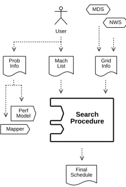
Fig. 1 presents the primary components of our scheduler and the interactions amongthose compo-nents. We provide this figure as a reference for the rest of the paper; we do not expect that all components or interactions will be completely clear at this point.
The Search Procedure is the core of the scheduler. This procedure is responsible for identifyingschedules that are appropriate to the target application and then selectingthe ‘‘best’’ one (Final Schedule in Fig. 1). A
schedule consists of an ordered list of machines and a mappingof application data or tasks to those machines. Before submittingan application to the scheduler, the user must currently obtain or develop the following application-specific components; eventually, we hope to
obtain these components automatically from the GrADS compiler.
* The performance model is a procedure that predicts application performance on a given set of resources. There are a variety of performance metrics that might be used for scheduling; in this section we assume that the performance model will predict application execution time.
* The mapper is a procedure that maps logical application data or tasks to physical resources. For each machine in the schedule, the mapper must define which piece of application data will be assigned to that machine. The mapper may choose a different orderingof machines than presented as input. These components are application-specific, but run-generic. In each application run, the user definesproblem parameterssuch as problem size. The performance model and mapper are then instantiated with this information to make them appropriate to the current problem run. We will describe several application-specific performance models and mappers in Section 3; in this section we simply assume that such components are available.
The user must also submit a machine list containing names of machines on which the user has an account; we forgo further discussion of this list until Section 2.4. For each machine in the machine list, we collect resource information such as CPU speed, available physical memory, and bandwidth between hosts. This informa-tion is retrieved from resource informainforma-tion providers such as the Network Weather System (NWS) and the Monitoringand Discovery Service (MDS); we discuss these services in Section 2.4.
2.2. Search procedure
To find good schedules, the search procedure first identifies groups of machines with both of the following qualities: (1) desirable individual machine characteristics and (2) desirable characteristics as an aggregate. For example, such groups would ideally be composed of computationally fast machines (an individual character-istic) and would be connected by low-delay networks (an aggregate characteristic). We call such groups of machines candidate machine groups(CMGs). The basic operations of the search procedure are then (i) identify CMGs; for each one (ii) call the mapper to find an appropriate application to machine mapping, and (iii) call the performance model to predict performance for the given CMG and mapping.
The most straightforward approach for the search for CMGs is an exhaustive search over all possible groups of machines. For many testbed sizes of interest (dozens of machines), such a search will introduce unacceptable schedulingoverheads and is therefore not a feasible solution. However, if the scheduler is going to provide reasonable application performance, it must identify CMGs that are reasonable for the application. There-fore, our search procedure uses extensive but careful pruningof the search space.
Pseudo-code for our schedule search procedure is given in Algorithm 1. In eachforloop the list of target CMGs is refined based on a different resource set characteristic: connectivity in the outer-most loop, computational and memory capacity of individual machines in the second loop, and selection of an appropriate resource set size in the inner-most loop. The goal is to generate only a moderate number of CMGs while ensuringthat we do not exclude performance-efficient CMGs. Final Schedule Grid Info Mach List Prob Info Mapper Perf Model User NWS MDS Search Procedure
The first step of our search procedure is to call the FindSites method; this method takes a list of machines and organizes them into disjoint subsets, or sites, such that the network delays within each subset are lower than the network delays between subsets. As a first implemen-tation, we group machines into the same site if they share the same domain name; we plan to consider more sophisticated approaches [31,37] in future work. The ComputeSiteCollections method computes the power set of the set of sites (we exclude the null set). As an example, for the set of sites fA;B;Cg; there are seven site collections: fA;B;C;A,B;A,C;B,C;A,B,Cg: Once all machine collections have been identified, the
outer-most loop of the search procedure examines each one in turn.
In the middle loop of the search procedure, we seek to identify machines that exhibit high local memory and computational capacities. Generally, we will not know a priori which machine characteristic will have the greatest impact on application performance; we therefore define three metrics that are used to sort
the machine list: thecomputation metric emphasizes the computational capacity of machines, the memory metric emphasizes the local memory capacity of machines, and the dual metric places equal weight on each factor.
The inner-most loop exhaustively searches for an appropriately sized resource group. Resource set size selection is complex because it depends on problem parameters, application characteristics, and detailed resource characteristics. Rather than miss potentially good resource set sizes based on poor predictions, we include all resource set sizes in the search. Note that an exhaustive search at this level of the procedure is only feasible due to the extensive pruningperformed in the first two loops. The SortDescending method sorts the input machine list collection by the machine character-istic machineMetric in descendingorder (the most desirable machines will be first). TheGetFirstNmethod call simply returns the firsttargetSizemachines from the sortedlist.
A key aspect of our approach is that no application-specific characteristics or components have been involved in the search procedure to this point. We have simply generated a large number of CMGs that could be of interest to applications in general.
Next, to evaluate each CMG, the Generate-Schedulemethod (1) uses theMapperto develop a data mappingfor the input CMG, (2) uses the Performance model to predict the execution time for the given schedule (predtime), and (3) returns a schedule structure which contains the CMG, the map, and the pre-dicted time. Finally, schedules are compared to find the schedule with the minimum predicted ex-ecution time; this schedule is returned as the
bestSched.
2.3. Search complexity
The most straightforward schedule search method is an exhaustive search; such a search is guaranteed to include the optimal CMG in those examined (note that pickingthe best one is dependent on an accurate performance model for any such search procedure). For a resource pool of sizep;an exhaustive search must examine 2pCMGs. For example, a schedule search for a 30 machine resource group would require evaluation of 230E109 CMGs. For a reasonably sized resource set
and/or when the performance model evaluation or mappingprocess is time intensive, an exhaustive search is simply too costly.
In the majority of cases, our search procedure provides an impressive reduction in search space. To demonstrate this we develop aloose upper bound on the number of CMGs considered by the search heuristic. Assumingwe have s sites in the resource set under consideration, we obtain 2s site collections (in fact, we exclude the null set leaving2s1 such collections). We consider three resource orderings for each collection (computation, memory, and dual). Given these 32s ordered collections, we exhaustively search all possible subset sizes for each. Since the number of resources in each site, and therefore in each topology-based collec-tion, is dependent on the characteristics of each Grid environment, we cannot predict a priori the number of resources in each of the 32sordered collections. As an upper bound, we assume each collection is of sizep;the size of the entire resource pool. Then, in the third loop of our search procedure, p distinct subsets will be generated for each ordered collection. The upper bound on the total number of CMGs identified by the search procedure is therefore 3p2s: Recall our earlier example of a 30 machine set; the exhaustive search required evaluation of 109 CMGs in this case. Supposingthis resource set included three sites, our search procedure would require evaluation of at most 720 CMGs. In fact, if we assume 10 machines in each of the three sites, our search procedure requires evaluation of only 360 CMGs. Our methodology provides a reduction in search space when the number of sites under consideration is significantly less than the number of machines; this is the case in the vast majority of modern Grids.
2.4. Use of Grid information
Grids are highly dynamic environments where com-pute and network resource availability varies and Grid information sources can be periodically unstable. We strive to provide best-effort service by supporting multiple information sources, when possible, for each type of information required by the scheduler.
We currently support information collection from the two most widely used Grid resource information
systems, the Monitoringand Discovery Service (MDS)
[12]and the Network Weather Service (NWS)[44]. The
MDSis a Grid information management system that is used to collect and publish system configuration, capability, and status information. Examples of the information that can typically be retrieved from an MDS server include operatingsystem, processor type and speed, and number of CPUs available. TheNWSis a distributed monitoringsystem designed to track and forecast resource conditions. Examples of the informa-tion that can typically be retrieved from an NWS server include the fraction of CPU available to a newly started process, the amount of memory that is currently unused, and the bandwidth with which data can be sent to a remote host.
Our schedulingmethodology can utilize several types of resource information: a list of machines available for the run, local computational and memory capacities for each machine, and network bandwidth and latency information. The list of machines is currently obtained directly from the user; once secure MDS publishing mechanisms are available, user account information can be published directly in the MDS and retrieved automatically by the scheduler. Local machine compu-tational and memory capacity data are used to sort machines in our search procedure and will be needed as input to many performance model and mapper im-plementations. Network bandwidth and latency data will similarly be required as input to many performance model and mapper implementations.
An important characteristic of our approach is that the scheduler gracefully copes with degraded Grid information availability. Whenever possible we support more than one source for each type of resource information required by the scheduler. Furthermore, when a particular type of information is not available for specific machines in the machine list, but is required by the scheduler, the scheduler excludes those machines from the search process. In our experience, most application schedulers do not gracefully handle such situations, leadingto many scenarios in which the scheduler fails.
3. Application case studies
In this section we describe specific applications that we used to demonstrate our schedulingmethodology in validation experiments; these experiments will be pre-sented in Section 4.
For each application, we develop a performance model that predicts both execution time and memory usage. We also present a strategy for comparing candidate schedules in the absence of an execution time model; this strategy demonstrates that our scheduling framework can be adjusted to accommodate alternative
performance metrics or types of performance model. We also implement two mappers that can be applied to our test applications: a time balance mapper, which can be used when an execution time model is available, and an equal allocation mapper, which can be applied when application information is limited to a memory usage model.
3.1. Case study applications
We have chosen applications from the class of regular, iterative, mesh-based applications as they are important in many domains of science and engineering
[16,17,22,6]. Specifically, we focus on the Game of Life
andJacobi. We have selected these applications as our initial test cases because they are well-known, straight-forward to describe, and share many performance characteristics with other applications.
Conway’s Game of Life is a well-known binary cellular automaton whereby a fixed set of rules are used to determine a next generation of cells based on the state of the current generation[16]. A two-dimensional mesh of pixels is used to represent the environment, and each pixel of the mesh represents a cell. In each iteration, the state of every cell is updated with a 9-point stencil. We use a 1-D strip data partitioningstrategy because this strategy typically exhibits lower communication costs than other partitioningschemes, an important consid-eration for Grid computing. Each processor manages a data strip and defines a 1-pixel wide set of ghost-cells alongdata Grid edges. Each iteration consists of a computational phase in which processors update their portion of the data array, and a communication phase in which processors swap ghost cell data with their neighbors.
TheJacobi methodis a simple algorithm that is often used in the context of Laplace’s equation [6]. Here we describe the general linear system solver version, which involves more communication (broadcasts). The method attempts to solve a square linear systemAx¼bwith the followingiteration formula: xkjþ1¼ 1 ajj bj X iaj ajixki ! ; ð1Þ where xk
j is the value of the jth unknown at the kth iteration. This method is guaranteed to converge only if matrixAis diagonally dominant.
We chose a popular parallel data decomposition for the Jacobi method whereby a portion of the unknown vector x is assigned to each processor; processors therefore need only store rectangular sub-matrices of
A:Each processor computes new results for its portion of x; and then broadcasts its updated portion of x to every other processor. The final phase in each iteration is a termination detection phase. The method is
stationary, meaningthat the matrix Ais fixed through-out the application.
We implemented each test application as a SPMD-style computation usingC and the Message Passing Interface (MPI) [33]. To allow load-balancingwe implemented support for irregular data partitions in both applications. We used the Globus-enabled version of MPICH[25], MPICH-G[18,26], in order to run over a Grid testbed.
3.2. Application performance modeling
Our schedulingframework is dependent on the availability of a performance model. The ScheduleCom-pare method described in the previous section assumes a performance model that predicts application execution time. Ultimately, such performance models may be automatically generated by the compiler in the GrADS framework. For the moment, we develop such a performance model for Jacobi and the Game of Life. We also develop a memory usage model, which will be required for the mapper discussion in Section 3.4.
Although both applications support rectangular data Grids, we assume that the full data mesh is a two-dimensional square. We use the followingdefinitions in the rest of this section. We refer to the size of either dimension of the data mesh asN;note that the number of data elements, and therefore the amount of work, grows as N2: We refer to the processors chosen for
execution as P0;y;Pp1 and the size of the data
partitions allocated to each processor asn0;y;np1: 3.2.1. Memory usage model
Given the magnitude of performance degradation due to paging of memory to disk, we must ensure that the application fits within the available memory of the processors selected for execution. We compute the amount of memory (in bytes) required for a data strip of sizeNnias
memReqi¼memUnitniN; ð2Þ where memUnitis the number of bytes of storage that will be allocated per element of the data domain. The Game of Life allocates two matrices of integers and Jacobi allocates one matrix of doubles. For the architectures we targeted in this paper, 4 bytes are allocated per integer and 8 bytes are allocated per double. Therefore, memUnit¼8 for both applications.
Recall that local processor memory availability,memi; can be supplied by total physical memory values from the MDS[12]or free memory values from the NWS[44]. In practice, a close match of memReqi and memi provides an overly tight fit due to memory contention with system or other user processes. Based on early experimental results and memory usage benchmarks,
increasing memReqi by 20% provides a reasonable tradeoff for the GrADS testbed environment[7].
3.2.2. Execution time model
Our test applications are dominated by regular, synchronous iterations; the application execution time can therefore be assumed proportional to the iteration time on the slowest processor. The iteration time on processor Pi is naturally modeled as the sum of a computation time and a communication time:
itTimei¼compTimeiþcommTimei: ð3Þ Thecomputation phasefor our test applications primar-ily consists of the data update process in each iteration and may include a termination detection operation (e.g. for Jacobi). We model computation time on processor
Pi as compTimei¼ compUnitniN 106comp i ; ð4Þ
where compUnit is the number of processor cycles performed by the application per element of the data domain. The computational capacity of processor Pi; compi;can be represented by raw CPU speed (from the MDS) and the currently available CPU (from the NWS), or a combination thereof. To fully instantiate this model, we need to determine an appropriate
compUnitvalue for each case study application. Rather than usingmethods such as source code or assembly code analysis, we opted for an empirical approach: we ran applications on dedicated resources of known CPU speed for 100 iterations and computed average
compUnitvalues.
TheGame of Life communication phaseconsists of the swapping of ghost cells between neighboring machines. We use non-blockingsends and receives, and, in theory, all of the messages in each iteration could be overlapped. In practice, however, processors cannot simultaneously participate in four message transfers at once without a reduction in performance for each message and, more importantly, processors do not reach the communica-tion phase of each iteracommunica-tion at the same moment. As an initial approximation, we assume that messages with a particular neighbor can be overlapped, but that com-munication with different neighbors occurs in distinct phases which are serialized.
TheJacobi communication phaseinvolves a series ofp
broadcasts per iteration; each machine in the computa-tion is the root of one of these broadcasts. In the MPI implementation we used in this work, the broadcast is implemented as a binomial tree [5]. As a first approx-imation to modelingthis communication structure, we calculate the average message time, msgTimeavg; and calculate the communication time on processorPias commTimei¼plog2ðpÞ msgTimeavg: ð5Þ
Our Game of Life and Jacobi communication models each depend on a model for thecost of sending a message
between two machines. We initially opted for the simple and popular latency/bandwidth model for a message sent fromPi toPj:
msgTimei;j¼latencyi;jþmsgSize=bandwidthi;j; ð6Þ where latency and bandwidth measurements and fore-casts are provided by the NWS. However, we observed that this model significantly over estimates the message transfer times of our applications. We found that a bandwidth-only modelðlatency¼0Þled to much better predictions. In the rest of the paper we use the more accurate bandwidth-only model.
3.3. Alternative performance models and metrics
In Section 2 we presented our schedulingmethodol-ogy with the assumption that an application-specific performance model would be available. What if one wanted to use a different performance metric or a different performance model? Due to the decoupled nature of our schedulingapproach, the only component that needs to be modified is the ScheduleCompare method implementation (seeFig. 1).
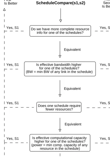
As an example, suppose a memory usage model is available, but an execution time model is not. The memory usage information will be used by the mapper (see Section 3.4) to ensure that candidate schedules fulfill application memory requirements. An alternative to a performance model for the purpose of schedule com-parisons is a series of heuristics that evaluate how well the candidate schedules satisfy a set of broad resource requirements such as bandwidth or computational capacity.Fig. 2presents a decision tree that implements such a series of simple heuristics. This decision tree is appropriate for Jacobi and the Game of Life and will be used in validation experiments in Section 4.
3.4. Application data mappers
The function of the mapper is to determine an appropriate mappingof work (i.e. strip widths
n0;y;np1) onto processors ðP0;y;Pp1Þ: The
map-pingprocess involves two distinct subproblems. The first problem is to determine a topological arrangement of machines (e.g. which physical processor should be assigned to logical processor position P0) such that
application communication costs are minimized. The second problem is to find an allocation of work to processors (e.g. how many rows of the data mesh should be assigned to process P0) such that application
resource-requirements are met and, when possible, application execution time is minimized.
In the followingsections we present two mappers: an equal allocation mapper and a time balance mapper.
3.4.1. Equal allocation mapper
In this mapper, work is simply allocated uniformly to all processors such that each is assigned an equally sized data strip of sizeN=pand the number of pixels assigned to each processor isNN=p:Before returningthis data map, the mapper verifies that each processor has sufficient local memory to support the application’s memory requirements. When at least one processor does not have sufficient memory, the mapper returnsfailure. In the schedulingcontext presented in Section 2, the current machine group is removed from the list of CMGs and the search process continues.
This mapper requires only a memory usage model and not a full execution time model. In production Grid schedulingsystems we expect there will be many applications for which a full performance model is not available. In such a case, our schedulingmethodol-ogy can still be applied by pairing it with the equal allocation mapper and the alternative performance
Do we have more complete resource info for one of the schedules?
Yes, S2 Yes, S1 Equivalent Return Second Is Better Return First Is Better
Is effective bandwidth higher for one of the schedules? (BW = min BW of any link in the schedule)
Yes, S1
Equivalent
Does one schedule require fewer resources?
Yes, S2
Is effective computational capacity higher for one of the schedules? (power = min comp. capacity of any
resource in the schedule)
Equivalent
Yes, S1 Yes, S2
Yes, S1 Yes, S2 Equivalent
ScheduleCompare(s1,s2)
Fig. 2. A schedule comparison approach for scenarios in which an application performance model is not available. Direct execution time comparisons are replaced by heuristic estimates of the desirability of proposed schedules.
model presented in the precedingsection. We explore such a scenario in Section 4.
3.4.2. Time balance mapper
For regular, synchronous iteration applications, application execution time is limited by the progress of the slowest processor. Total execution time can be minimized by (1) findingan orderingof machines such that the need for wide-area messages is minimized and (2) findinga data map for which all processors complete their work in each iteration at the same time, thereby minimizingsynchronization times. The goal of the time balance mapper is to find such a data map while ensuringthat application memory requirements are met.
Our approach to problem (1) is to reorder the input machines such that machines from the same site are adjacent in the topology. Since the Game of Life is dominated by neighbor-based communications, this orderingis highly effective for reducingcommunication costs for that application; its effectiveness is less clear for Jacobi which is dominated by all-to-all broadcasts. One can think of more sophisticated approaches for reorderingmachines; for this work we focused more on problem (2).
For problem (2), our approach is to formalize machine resource availabilities, application memory requirements, and execution time considerations as a series of constraints. Work allocation can then be framed as a constrained optimization problem; the solution is a map of data strip widths to processors. We first describe the general operation of the mapper, and then describe our formalization of the problem.
When called, the time balance mapper first verifies that the aggregate memory of the CMG is sufficient for the aggregate requirements of the current application problem. If not, the mapper does not attempt to find a data map and returns a failure. If the CMG has sufficient aggregate memory, the mapper searches for a perfectly time-balanced data map; if found, the map is returned. Sometimes, one or more machines do not have sufficient local memory to satisfy the memory require-ments of a perfectly time-balanced map. In this case, the mapper relaxes the time balance constraints to seek a less well-balanced map that can satisfy memory require-ments. The mapper uses a binary search to find the map that provides the best time balance while satisfying application memory requirements. The parameters of the binary search are configurable; default values are provided as follows. The default maximum relax factor is 10, meaningthat, at worst, predicted iteration time on the slowest processor is no more than 10 times the predicted iteration time on the fastest processor. The default search tolerance is 0.01, meaningthat the search refinement ends when the relax factor changes by less than 0.01 between search steps.
We now briefly describe our specification of this problem as a constrained optimization problem; see[13]
for a thorough explanation and [15,39] for previous work that applied a similar solution for other data mappingproblems. The unknowns are the strip widths to be assigned to each processor:n0;y;np1:Since strip widths are constrained to integer values, the problem can be framed as an integer programming problem[43]. Unfortunately, the integer programming problem is NP-complete, renderingthe solution computationally ex-pensive to compute and unacceptable for use in our schedulingmethodology. We use the more efficient alternative of real-valued linear programming solvers
[43] (specifically, we use the lp solve package which is based on the simplex method). Although using a real-valued solver for an integer problem introduces some error, the resultingaccuracy is sufficient for our needs.
The problem formulation begins with the specification of anobjective function. Since it is impossible to express our true objective in a linear formulation, we instead minimize the computation time onP0 (see Section 3.2.2
for our computation time model); later we specify constraints that ensure the other processors are time-balanced with P0: Next, we specify bounds on the
unknown variables: each processor should be assigned a non-negative number of mesh rows not to exceed the total number of rowsN:8iAf0:p1g;0pnipN:The rest of the specification is in the form of constraints. First, the total number of data mesh rows allocated must be equal to N: Ppi¼01 ni¼N: Next, the data allocated to each processor must fit within that processor’s local memory: 8iAf0:p1g;memUnit Nnipmemi; refer to Section 3.2.1 for our memory usage model. Finally, we specify that each processor’s predicted iteration time should equal P0’s predicted
iteration time: 8iAf1:p1g;jitTimeiitTime0j ¼0: We add support for relaxation of time balanc-ingrequirements with relax factorRand the constraint becomes: 8iAf1:p1g;jitTimeiitTime0jpR itTime0:After incorporatingdetails from our execution
time model (see Section 3.2.2), re-arranging, and using two inequalities to specify an absolute value, our last two constraints are
8iAf1:p1g;ð1þRÞ compTime0þcompTimei pð1þRÞ commTime0commTimei; ð7Þ 8iAf1:p1g;ð1RÞ compTime0compTimei
pð1þRÞ commTime0þcommTimei: ð8Þ 3.5. Application component validation
As described in Section 2, our scheduler typically utilizes a performance model to compare candidate schedules. The ability of our scheduler to select
the ‘‘best’’ schedule is therefore directly tied to the prediction accuracy of the performance model. To provide backingfor the usage of our performance models in the scheduler validation experiments (Section 4), we describe here a suite of validation experiments for the execution time model we described in Section 3.2. The goal of these experiments was to compare predicted application performance (predTime) with actual appli-cation performance (actualTime). We calculate the prediction error as
predError¼100predTimeactualTime
actualTime : ð9Þ
We do not have space here to fully describe our experimental design; a full explanation is available in
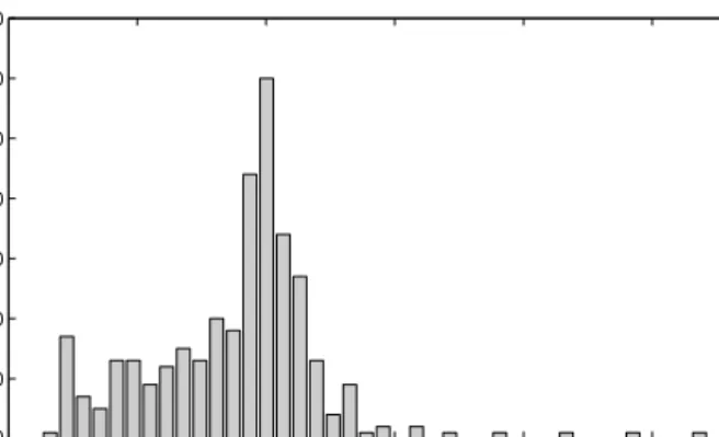
[13]. We tested model accuracy for the Jacobi and the Game of Life applications on a one site testbed and a three site testbed (see Section 4.1 for details). In total, we obtained 344 comparisons of actual and predicted times. A histogram of the prediction errors we measured in those experiments is shown inFig. 3.
The prediction accuracy of our execution time model is moderate. The objective of this work is not to provide performance models for applications, but rather to demonstrate how such models can be utilized as part of our schedulingstrategy. More sophisticated and precise models could be developed and used. Our evaluation results will show how our approach behaves with reasonably accurate models. Such are the models we hope to obtain automatically from the GrADS compiler when it becomes available.
4. Results
In this section we describe experimental results obtained for the Jacobi and Game of Life applications
in realistic Grid usage scenarios. We designed these experiments to investigate the following questions.
(i) Does the scheduler provide reduced application execution times relative to conventional scheduling approaches?
(ii) Can the scheduler effectively utilize dynamic resource information to improve application performance? Can reasonable schedules still be developed in the absence of dynamic resource information?
(iii) How is scheduler behavior affected by degraded application information? Specifically, can reason-able schedules still be developed in the absence of an application execution time model?
Our previous work in application-level schedulers[8]has demonstrated success with questions (i) and (ii) in the context of specific applications or applications classes; we will discuss those results in Section 5. The challenge in our current work is to employ an application-generic schedulingapproach to achieve these goals.
4.1. Experimental design 4.1.1. Testbeds
Our experiments were performed on a subset of the GrADS testbed composed of workstations at the University of Tennessee, Knoxville (UTK), the Univer-sity of Illinois, Urbana-Champaign (UIUC), and the University of California, San Diego (UCSD). Fig. 4
depicts our testbed and provides a snapshot of available bandwidths on networks links. Table 1 summarizes testbed resource characteristics. This collection of resources is typical of Computational Grids: it is used by many users for an array of purposes on an everyday basis, the resources fall under a variety of administrative domains, and the testbed is both distributed and heterogeneous.
Experiments were performed on the full three-site tested and on a one-site testbed with only UCSD resources. We ran experiments on the one-site testbed withproblem sizesoff600;1200;2400;4800;7200;9600g and on the three-site testbed with problem sizes of f600;4800;9600;14400;16800;19200g: This range of problem sizes covers a broad range of application resource requirements: a size of 600 requires only 3 MB and can run on a single machine, while a size of 19,200 requires over 3 GB and must be allocated most of the three-site testbed before a satisfactory data mappingcan be found.
4.1.2. Scheduling strategies
To help answer questions (i)–(iii), we developed four schedulingstrategies, dynamic, static, basic, and user, each based on a realistic Grid schedulingscenario. The dynamic strategy uses our scheduler design and
-1000 -50 0 50 100 150 10 20 30 40 50 60 70
Percent prediction error
Samples
Fig. 3. Histogram of prediction errors measured in a total of 344 experiments. Results are aggregated from experiments conducted with Jacobi and the Game of Life on both a single site testbed and a three site testbed.
represents the case when full information is available about the application and testbed. For this strategy, the scheduler is coupled with the full execution time performance model (see Section 3.2.2) and time balance mapper (see Section 3.4.2). Schedulingdecisions are made at run-time and are based on near real-time CPU availability, free memory, and available bandwidth information from the NWS as well as CPU speed data from the MDS.
The static strategy models our scheduler’s behavior when full application information is available, but
resource information is degraded. Specifically, this strategy uses the same performance model and mapper as the dynamic strategy, but assumes dynamic resource information is not available at run-time (i.e. the NWS server is unavailable). Schedulingdecisions are made off-line, and are based on static information from the MDS such as available physical memory and total CPU speed. Estimates of available bandwidth from the NWS are used, but are not collected at run-time.
The basic strategy models our scheduler’s behavior when resource information is fully available, but a complete execution time model is not. This strategy uses the memory usage model described in Section 3.2.1, the equal allocation mapper defined in Section 3.4.1, and the alternative ScheduleCompare method defined in Section 3.3. None of these components require execution time information.
Since sophisticated schedulers are not widely available for Grid computing, user-directed scheduling is the ‘‘standard’’ or ‘‘conventional’’ method. We therefore developed a user strategy to emulate the scheduling process that a typical Grid user might employ. We assume that users will generally only invest time in schedulingonce per application configuration; in this scenario static resource information is sufficient since schedulingoccurs off-line. We also assume that a user has a preferred orderingof resources; for example, most users will utilize their ‘‘home’’ resources before resources on which they are a ‘‘guest’’. For the three-site testbed, we assume a resource orderingoffUCSD;UTK;UIUCg: We assume a typical user will not have a detailed performance model, but may be able to estimate
UTK LAN 83.8 Mbps UIUC-M LAN 88.6 Mbps UCSD LAN 90.8 Mbps 4.4 Mbps 2.7 Mbps 3.0 Mbps 1.5 Mbps 6.0 Mbps 5.9 Mbps WAN UIUC-O LAN 88.6 Mbps
Fig. 4. A heterogeneous, distributed network of workstations. Net-work links are labeled with available bandwidth in megabits per second; these values were collected by Network Weather Service network monitoringsensors on November 1, 2001 at around 5:30 PM.
Table 1
Summary of testbed resource characteristics
Name Circus (UCSD) Torc (UTK) Opus (UIUC) Major (UIUC)
Domain ucsd.edu cs.utk.edu cs.uiuc.edu cs.uiuc.edu
Nodes 6 8 4 6
Names dralion, mystere, soleil torc1, torc2, torc3, torc4 opus13-m, opus14-m amajor, bmajor, cmajor quidam, saltimbanco, nouba torc5, torc6, torc7, torc8 opus15-m, opus16-m fmajor, gmajor, hmajor
Processor 450 MHz PIII 550 MHz PIII 450 MHz PII 266 PII
dralion, nouba 400 MHz PII
others
CPUS Per Node 1 2 1 1
Memory Per Node 256 MB 512 MB 256 MB 128 MB
OS Debian Linux Red Hat Linux Red Hat Linux Red Hat Linux
Kernel 2.2.19 2.2.15 SMP 2.2.16 2.2.19
Network 100 Mbps 100 Mbps 100 Mbps 100 Mbps
application memory usage. The strategy therefore uses our memory usage model and selects the minimum number of resources that will satisfy application memory requirements. Fig. 5 summarizes the applica-tion and Grid informaapplica-tion usage by each of the four schedulingstrategies.
Comparison of our scheduler against the performance achieved by an automated, run-time scheduler would clearly be a desirable addition to the four strategy comparisons we have defined. Unfortunately, there is currently no comparable Grid scheduler that is effective for the applications and environments that we target. We listed other Grid scheduler efforts in Section 1; we plan to investigate other applications and environments for which a reasonable comparison of our approach and some of those approaches could be made.
4.1.3. Experimental procedure
A schedulingstrategy comparison experiment consists of back-to-back runs of the application as configured by each schedulingstrategy. In each application execution, 104 iterations were performed; an average and standard deviation of the iteration times was then taken of all but the first 4 ‘‘warmup’’ iterations. Based on the character-istics of iterative, mesh-based applications, we compare application performance based on the worst average iteration time reported by any processor in the computation.
To avoid undesirable interactions between each application execution and the dynamic information used by the next scheduler test, we included a 3-min sleep phase between tests. To obtain a broad survey of relative strategy performance, we ran scheduling strat-egy comparison experiments for all combinations of the two applications, the two testbeds, and six problem sizes ð226¼24 testingscenariosÞ: We performed 10 repetitions of each testingscenario for a total of 240
scheduler comparison experiments and 720 scheduler/ application executions.
4.1.4. Strategy comparison metric
Our experiments included a large range of problem sizes, resulting in a very large range of iteration times. Aggregating such results via a straight average over emphasizes the larger problem sizes. Instead, we employ a common scheduler comparison metric,percent degra-dation from best [29]. For each experiment we find the lowest average iteration time achieved by any of the strategies,itTimebest; and compute
degFromBest¼100itTimeitTimebest
itTimebest
; ð10Þ for each strategy. The strategy that achieved the minimum iteration time is thus assigneddegFromBest¼ 0: Note that an optimal scheduler would consistently achieve a 0% degradation from best.
4.2. Aggregate results
Fig. 6presents an average of the percent degradation from best achieved by each schedulingstrategy across all schedulingstrategy comparison experiments. Each bar in the graph represents an average of approximately 70 values.Table 2presents additional statistics for the same data set. In all application-testbed combinations, the user strategy is outperformed, on average, by the three other strategies. Since all but the user strategy are variations of our schedulingmethodology, these results provide sufficient evidence to answerquestion (i) in the affirmative: our approach does provide reduced applica-tion execuapplica-tion times relative to a convenapplica-tional ap-proach. The improvement in average performance from the user to the static strategy partially answersquestion
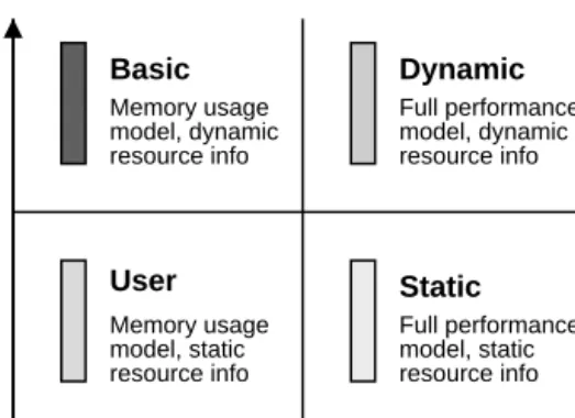
(ii): reasonable schedules can still be developed in the absence of dynamic resource information. Additionally, recall that the primary difference between the user and Sophistication of Application Information Sophistication of Resource Information User Basic Static Dynamic Memory usage model, dynamic resource info Full performance model, dynamic resource info Memory usage model, static resource info Full performance model, static resource info
Fig. 5. Summary of user, basic, static, and dynamic scheduling strategies. For each strategy we note the availability of sophisticated application and resource information. Shadingof bars corresponds to shading used for each strategy in the scheduling results graphs.
0 100 200 300 400
Percent degradation from best
Game of Life Game of Life Jacobi Jacobi One-site Three-site One-site Three-site
User Basic Static Dynamic
Fig. 6. Average percent degradation from best for each scheduling strategy and each application-testbed combination. Each bar repre-sents an average result for about 70 experiments.
basic strategy pair and the static and dynamic strategy pair is the usage of dynamic information. Since the basic strategy outperforms the user strategy and the dynamic strategy outperforms the static strategy, we can answer the rest ofquestion (ii) in the affirmative: the scheduler does effectively utilize dynamic resource information to improve application performance. Finally, in question
(iii) we asked how scheduler behavior is affected by the availability of an accurate performance model. As expected, the schedulingstrategies that utilize an accurate application performance model (static and dynamic) outperform those that do not (user and basic). While the schedulingstrategies show a clear ordering in average performance, examination of individual experimental results shows that relative scheduler performance can be heavily influenced by run-time conditions, application characteristics, and other fac-tors. In the followingsections, we present a detailed analysis of a small subset of our experiment results. We use these case studies to provide insight as to the behavior of each scheduling strategy, and to highlight conditions where a specific strategy was particularly effective or ineffective.
4.3. Case study I: variability with time
We first detail experimental results for the Jacobi application on the three-site testbed with a problem size of 9600. As with all experiment configurations, we performed 10 experiment repetitions. Specifically, we collected repetitions 1–3 on October 16–17, 4–6 on November 6–7, and 7–10 on November 9–10. In this section, we present the resource selection decisions made by each schedulingstrategy, and then describe applica-tion performance results obtained for these schedules.
Fig. 7reports the schedules selected by each schedul-ingstrategy in each experiment repetition. The location and number of machines selected is shown with grayed
rectangles. Machine selection is reported for each site in the testbed with UIUC machines further differentiated into the Opus cluster (labeledUIUC-O) and the Major cluster (labeled UIUC-M). In 38 of the 40 schedules shown in Fig. 7 the schedule includes machines from only a single site. While the user strategy is constrained to select machines in a particular order, the other strategies evaluated performance tradeoffs and auto-matically selected a subset of the total resource pool.
Fig. 7also shows that the user and static strategies each used the same schedule for all repetitions; this is because schedulingis done off-line with static information and such decisions do not vary across repetitions. By comparison, the basic and dynamic strategies each employed different schedules from repetition to repeti-tion; this is because the basic and dynamic strategies utilize dynamic information to make run-time schedul-ingdecisions. Notice also that the static and dynamic strategies typically select more machines than do either the user or basic strategies. The dynamic and static strategies select a resource set size that minimizes predicted application execution time; since the user and basic strategies model situations where an execution time model is not available, these strategies try to reduce communication costs by selectingthe minimum number of resources that satisfy application memory require-ments.
An interestingcharacteristic of Fig. 7 is that UTK resources are so frequently chosen, particularly by the static and dynamic strategies. In this testbed, theUTK site includes a substantial number of machines (8), each of which is more powerful (in terms of memory and computation) than any machine provided by the other sites (seeTable 1). TheUTKmachines are clearly a good choice when eight machines are sufficient for the current problem run. Note, however, that when the dynamic strategy selected more than eight machines (repetition 1 and 2), it did not includeUTKmachines in the schedule. In fact, throughout the time we were running the experiments for this paper we found that WAN performance between UTK and either UCSD or UIUC was significantly worse than WAN performance be-tweenUCSDandUIUC. For example, in repetition 4 of the current series (Jacobi application on the three-site testbed with a problem size of 9600) the dynamic scheduler obtained the followingbandwidth predictions from the NWS: UTK to UIUC 0.21 Mbps, UTK to UCSD 0.14 Mbps and UIUC to UCSD 5.92 Mbps. Accordingly, our scheduler (as represented by the basic, static, and dynamic strategies) automatically avoids schedules that use UTK machines in a multi-site schedule.
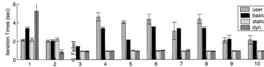
Fig. 8 reports results obtained when the application was executed with each of these schedules. In this figure, bar height indicates average iteration times across a single application execution, and error bars indicate
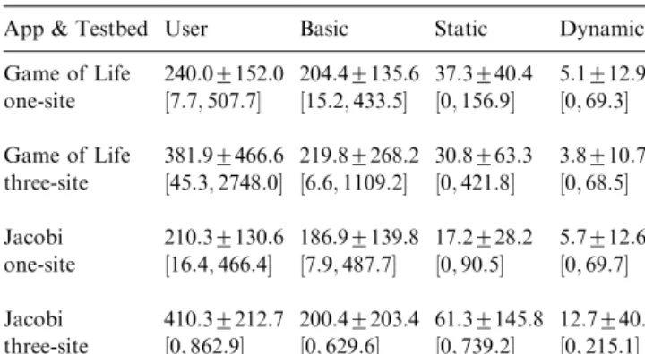
Table 2
Summary statistics for percent degradation from best for each schedulingstrategy over all application-testbed scenarios. In each cell the top line reports fAverage7Standard deviationgand the bottom line reportsfmin;maxg:
App & Testbed User Basic Static Dynamic Game of Life 240:07152:0 204:47135:6 37:3740:4 5:1712:9 one-site ½7:7;507:7 ½15:2;433:5 ½0;156:9 ½0;69:3 Game of Life 381:97466:6 219:87268:2 30:8763:3 3:8710:7 three-site ½45:3;2748:0 ½6:6;1109:2 ½0;421:8 ½0;68:5 Jacobi 210:37130:6 186:97139:8 17:2728:2 5:7712:6 one-site ½16:4;466:4 ½7:9;487:7 ½0;90:5 ½0;69:7 Jacobi 410:37212:7 200:47203:4 61:37145:8 12:7740:6 three-site ½0;862:9 ½0;629:6 ½0;739:2 ½0;215:1
standard deviation of iteration times. By comparingthe results of Fig. 8 with those of Fig. 6 we see that, as expected in real-world experiments, the results of individual experiments do not always follow the trends we see in average results.
No times are reported for the user strategy in the third repetition because the application failed to complete. Upon closer examination, we found that the size of the data allocated to one of the machines exceeded its available physical memory, leadingto serious interfer-ence with other users’ jobs. The application was killed to allow normal progress for the other jobs. This experi-ment highlights the importance of run-time scheduling with dynamic resource information.
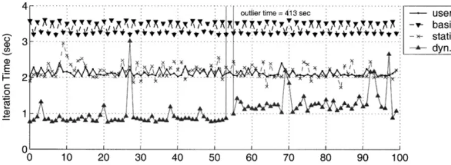
The results shown for the first repetition inFig. 8are striking. In this repetition, the dynamic strategy performed particularly poorly on average, and the standard deviation in iteration times was surprisingly high ð41:2 sÞ: Fig. 9shows the time measured for each iteration of the application in each of the four scheduler/ application runs in the first experiment repetition. The iteration times for each scheduler are plotted on the same graph for comparison purposes only; the applica-tion runs were actually performed at different times and, possibly, under different conditions. We have selected this case study for its usefulness in demonstratinga few points; the behavior of the schedulingstrategies seen here is in fact anomalous (refer toFig. 6).
While the dynamic strategy was the worst performer on average in this repetition, Fig. 9 shows that the dynamic strategy was actually the best performer for the majority of iterations and that a few dramatic iteration
time jumps were responsible for poor average perfor-mance. We investigated system behavior during the most dramatic jumpð413 sÞ;and found that NWS CPU availability measurements for bmajor.cs.uiuc.edu, one of the machines in this schedule, were almost completely missingduring320 s of the 413 s iteration. We believe that duringthe longiteration period bmajor.cs.uiuc.edu was completely off-line or so disrupted that even lightweight NWS sensors, and therefore our application, could not run. We also identified a correlation between a dramatic increase in bmajor.cs.uiuc.edu computation times duringthe last 40 or so iterations, and the broad shift upward in application iteration times in the last 40 or so iterations. This case demonstrates how sensitive the overall performance of even loosely synchronous applications can be to the performance of individual machines. This case also reveals the insights one can miss by examiningonly average iteration times; how-ever, average iteration times are representative of total execution time, an application metric of primary importance to users.
4.4. Case study II: variability with problem size
In the precedingcase study, we examined variations in scheduler behavior and performance across different repetitions of the same experiment. In this section, we again focus on experiments for the Jacobi application on the three-site testbed, but we detail experiments per-formed duringa shorter time period (5 h on November 4, 2001) and across a variety of problem sizes.Fig. 10
reports the machine selections used by each scheduling
Fig. 7. Processor selections for each scheduling strategy for the Jacobi application on the three-site testbed, problem size of 9600. For each experiment repetition, the processors selected by each strategy are highlighted with gray boxes.
strategy in these experiments, and Fig. 11 reports the measured application performance for each schedule. The iteration times reported inFig. 11extend from 0.01 to 20:68 s per iteration, a range of three orders of magnitude.
Notice that while all four strategies were successful in findinga schedule forN¼19200 (seeFig. 10), both the user and dynamic strategies failed during the launch or execution of the application itself (see Fig. 11). The dynamic strategy experiment failed during application launch due to an unidentified problem on the launching machine. The user strategy experiment failed because the application heavily interfered with a user’s work, who then killed the application. When the application interferes with the work of other users to this extent it suggests that (1) best estimates of available memory should be used at run-time to ensure the availability of
sufficient memory for the application and (2) our memory usage model may be too conservative in its estimate of how much memory should be available for the application on each machine. From the scheduling perspective, there must be an appropriate balance between selectingmore machines to provide enough memory for the application and selectingless machines to reduce communication costs.
There are four schedules shown inFig. 10that include both UTK machines and machines at another site: the user strategy for N¼14400;16800; and 19200 and the basic strategy for N¼19200: These cases correspond exactly to the worst iteration time results shown inFig. 11; these schedules performed poorly because of the poor network performance betweenUTKand the other sites (refer to the precedingsection for details). Since the orderingof machine selection is predefined for the user
Fig. 9. Time for each application iteration as a function of iteration number. Each run was performed at a different time and possibly under different conditions; they are plotted together for comparison purposes only. Results are for the Jacobi application on the three-site testbed withN¼9600 and repetition¼1: The dramatic drop is performance of the dynamic strategy at iteration 53 is responsible for that strategy’s poor average performance in repetition 1 ofFig. 8.
Fig. 10. Processor selections for each scheduling strategy for the Jacobi application on the three-site testbed for all six problem sizes. For each experiment repetition, the processors selected by each strategy are highlighted with gray boxes.
strategy fUCSD;UTK;UIUCg; it is not surprising that the user strategy selected these schedules. It is surprising, however, that the basic strategy selected such a schedule.
Let us investigate this behavior in some detail. A problem size of 19,200 is demandingfor this testbed; in aggregate, at least 3375 MB of RAM are required. Given an equal work allocation, this translates into per machine available memory requirements, for example, of 140:6 MB/machine for 24 machines, 210:9 MB/ machine for 16 machines, or 421:9 MB/machine for eight machines. Given unloaded conditions and an equal work allocation, a schedule for N¼19;200 cannot utilize all 24 machines because the major machines at UIUC have only 127 MB each, 16 machines can be utilized only if the major machines are excluded, and eight machine can be utilized only if all eight machines are fromUTK.
Notice that the basic strategy selected 16 machines. Since the basic strategy selects the smallest resource set that satisfies application memory requirements, it may seem surprisingthat the strategy selected more than just the 8 Torc machines. Recall however that the basic strategy collects and uses dynamic resource information at schedule-time (i.e. run-time). In this experiment, the basic strategy found that some of the UTK machines were partially loaded and could no longer provide the minimum 421:9 MB/machine needed to run the applica-tion on just the 8UTKmachines. The strategy therefore selected more machines, thereby reducingthe minimum memory required per machine to levels that could be supported by theUTKmachines.
Lookingagain at Fig. 10, it may now seem strange that both the static and dynamic strategies determined that an 8 UTK machine was an acceptable choice. The static strategy uses only static information and therefore assumes all resources are unloaded; under unloaded conditions the 8 UTK machines are an appropriate choice. Lookingat the results shown in Fig. 11, it appears that this choice was also reasonable in the conditions experienced by the static strategy (i.e. the strategy performed reasonably). In other cases, blindly assumingunloaded conditions can have drastic affects.
When the dynamic strategy ran, it retrieved run-time resource information and found that theUTKmachines were partially loaded. However, usage of the time balance mapper provided this strategy with the added flexibility of unequal work allocations. The time balance mapper found a map which allowed usage of the 8UTK machines by shiftingsome work from the partially loaded machines to the unloaded machines. In general, we found that the time balance mapper was not only generally successful in reducing application iteration times, but was also very useful in increasingthe number of schedulingchoices available.
4.5. Scheduling overhead
A scheduler design is practical only if the overhead of the schedulingprocess is reasonable when compared to application execution times. The overheads associated with our approach are highly dependent on the configuration of the scheduler; for this reason, we did not include the overheads of the schedulingprocess itself in the precedingexperiments. Rather, we examine the overhead of our approach with a variety of configura-tions in detail here.
We consider the total overhead for scheduling, as well as the overhead for each of the two activities performed by our schedulingmethodology: (i) the collection of resource information from the MDS and NWS and (ii) the search for candidate schedules. We measured schedulingoverheads for the Jacobi application on the three-site testbed with the same scheduler configuration as was used for the dynamic schedulingstrategy. While this case study provides a reasonable overview of the overheads of our methodology, note that the cost of schedulingis dependent on problem run configuration, the selected testbed, the target application, the complex-ity of the chosen performance model and mapper, and variable load on the GrADS NWS nameserver and MDS server.
It is important to differentiate the costs of data retrieval from the MDS and NWS servers from the cost of transferringthe request for data and the response over WANs. We set up an NWS nameserver and an MDS cache atUCSDand we performed the tests from a machine atUCSD; these sources of information will be referred to as thelocal NWSand thelocal MDS cache. We include test scenarios in which NWS information is retrieved from either the local NWS or from the GrADS NWS, which was located at UTK in Knoxville, Tennessee. We also include scenarios in which MDS information is retrieved from the local MDS cache or from the GrADS MDS, which was located atISIin Los Angeles, California. Specifically, we test the following retrieval modes.
* Mode A used the GrADS NWS nameserver and the GrADS MDS server.
* Mode B used the GrADS NWS nameserver and a local MDS cache. For these experiments, the local MDS cache contained all needed information (i.e. it wasfully warmed).
* Mode C used the local NWS nameserver and a fully warmed local MDS cache.
We ran the scheduler with each of the three retrieval modes in a back-to-back manner; we completed 10 such triplets. For each run, we measured the time required for the entire schedulingexecution (TotalTime) and the time required for Grid information collection ( Collect-Time); we consider the cost for the schedule search
(SearchTime) to be all schedulingtime that is not spent in information collection: SearchTime¼TotalTime
CollectTime:
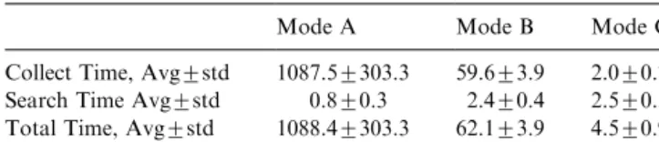
Table 3 presents summary results over all 10 repeti-tions for the mean and standard deviation of the
CollectTime, SearchTime, and the TotalTime. For reference, when we ran schedulingexperiments with a similar experimental configuration, the four scheduling strategies typically achieved application iteration times between 1.8 and 11 s: Since we ran roughly 100 iterations in these experiments, the application’s itera-tive phase occupied 180–1100 s:
The cost of Grid information collection dominates schedulingoverhead in all modes except C. In mode C only 2 s; on average, were required to collect informa-tion on all 24 machines in this testbed. This overhead is very reasonable when compared with application run-times; we conclude that our procedure for collecting resource information is efficient enough and that the cost of data retrieval from an NWS server is reasonable. In mode B, NWS data were retrieved from a remote NWS server, which increased information collection times to approximately 60 s:We conclude that collection of information from a remote NWS server is efficient enough for most uses of our scheduler. The overhead could become problematic for a larger testbed; in this case, our scheduler can be used without run-time resource information as was done for the static strategy in this paper. Finally, mode C utilized both the remote NWS nameserver and the remote MDS server, thus increasingcollection times to 1087:5 s;or approximately 18 min: This overhead is prohibitive, and, in practice, would prevent usage of our scheduling approach. We conclude that until retrieval times are reduced for the MDS, local cachingof MDS information will be necessary. The MDS information that is retrieved and used by our methodology changes on the order of weeks or months; local cachingis therefore an acceptable solution for this work. Note that ongoing development work in both MDS and NWS is seekingto reduce information retrieval latencies.
The cost of the schedule search process is less than 2:5 s for all three collection modes and is therefore an acceptable overhead for our schedulingscenarios. This low search time overhead is due to (1) the low computational complexity of our execution time model and mappingstrategy and (2) the extensive search
pruningperformed duringthe search process. Notice that the average search time in mode A is only about 33% of the search time for modes B and C. Mode A retrieves some resource information from the GrADS MDS and duringthese experiments that server was unable to provide much of the required information. Our schedulingmethodology does not consider ma-chines for which no data is available, thus leadingto pruningof the schedule search space and a reduction in search time.
4.6. Usability
Our schedulingapproach is an integrated component of GrADSoft, the prototype GrADS system. Other members of the GrADS project have applied this prototype (and therefore our scheduler) to three diverse and important applications: FASTA [23] (protein and genome sequence alignment), Cactus[22](a framework for computational physics), and ScaLAPACK LU Solver[21] (a solver for dense systems of equations via LU factorization).
For all three applications, it seems that usingour schedulingapproach was straightforward. The most difficult aspect is, perhaps, developinga performance model and mappingstrategy by hand for each applica-tion. In the longterm we expect to obtain such components automatically from the GrADS compiler; in the meantime, for Cactus and ScaLAPACK, usage of our approach was quite straightforward since a perfor-mance model had already been developed for prior GrADS work and a very simple mappingstrategy was easily developed (equal allocation for both Cactus and ScaLAPACK). For FASTA, the developer had to create both a performance model and mappingstrategy but, once these were available, the scheduler was easily applied for this application as well.
In our experiences with Application-Level Schedulers (AppLeS) targeted for specific applications, we did not reuse our own schedulers for new applications and we did not provide the software to other groups for their own usage. The integrated application/scheduler combi-nations were clearly effective for the original applica-tion, but the designs were not general enough to reapply in new circumstances. The application of our approach by other researchers to new applications indicates that our decoupled design did indeed result in an easier to use, retargetable scheduler.
5. Discussion
In this section we summarize the scope of the work (Section 5.1), describe related work (Section 5.2), describe possible extensions to our work (Section 5.3), and conclude the paper (Section 5.4).
Table 3
Schedulingoverheads in seconds to schedule Jacobi on the three-site testbed,N¼14400, dynamic schedulingstrategy
Mode A Mode B Mode C Collect Time, Avg7std 1087.57303.3 59.673.9 2.070.7 Search Time Avg7std 0.870.3 2.470.4 2.570.3 Total Time, Avg7std 1088.47303.3 62.173.9 4.570.9