Entrainment-Mixing and Radiative Transfer Simulation in Boundary Layer Clouds
FRÉDÉRICKCHOSSON ANDJEAN-LOUIS BRENGUIER
Météo-France, CNRM/GMEI, Toulouse, France
LOTHAR SCHÜLLER
EUMETSAT, Darmstadt, Germany
(Manuscript received 9 February 2006, in final form 9 November 2006) ABSTRACT
In general circulation models, clouds are parameterized and radiative transfer calculations are performed using the plane-parallel approximation over the cloudy fraction of each model grid. The albedo bias resulting from the plane-parallel representation of spatially heterogeneous clouds has been extensively studied, but the impact of entrainment-mixing processes on cloud microphysics has been neglected up to now. In this paper, this issue is examined by using large-eddy simulations of stratocumulus clouds and tridimensional calculations of radiative transfer in the visible and near-infrared ranges. Two extreme scenarios of mixing are tested: the homogeneous mixing scheme with constant concentration and reduced droplet sizes, against the inhomogeneous mixing scheme, with reduced concentration and constant droplet sizes. The tests reveal that entrainment-mixing effects at cloud top may substantially bias the simulated albedo. In the worse case, which corresponds to a fragmented and thin stratocumulus cloud, the albedo bias changes from⫺3% to⫺31% when using both mixing schemes alternatively.
1. Introduction
The parameterization of clouds and of their radiative properties in general circulation models (GCMs) re-mains a challenge because of the coarse horizontal and vertical resolutions of the models. With a horizontal resolution of the order of 100 km, model grids are likely to be partially filled with clouds. The relationship be-tween cloud optical thickness, that depends on the liq-uid water path (LWP), and cloud albedo however is nonlinear. The cloud albedo derived by assuming that LWP is uniformly distributed over the whole grid area is larger than if LWP is restricted to a prescribed frac-tion of the grid. It is therefore crucial to correctly di-agnose both LWP and at least the cloud fraction (CF), for example, based on a predicted probability density function (PDF) of a quantity related to the water vapor saturation in the grid (Larson et al. 2001). At specified LWP and CF, cloud radiative properties also depend on
the size distribution and optical properties of the cloud particles. Hence, Twomey (1977) hypothesized that, in liquid water clouds, an anthropogenic increase of the number concentration of cloud condensation nuclei (CCN) would result in an increase of the cloud droplet number concentration (CDNC) and, at constant LWP, in an increase of the cloud albedo. This process is re-ferred to as the first aerosol indirect effect (AIE).
In GCMs, cloud radiative transfer simulations are currently performed by assuming that the cloud is a horizontally uniform layer, with the specified LWP, covering a fraction CF of the model grid. This is re-ferred to as the plane-parallel model (PPM). Cloud par-ticles’ optical properties are derived from a prescribed drop size distribution by assuming that the cloud layer is either vertically uniform (VUPPM model), or using a more realistic scheme for convective clouds, in which the liquid water content (LWC) increases with altitude following an adiabatic profile (ASPPM model; Bren-guier et al. 2000).
The impact of the subgrid spatial variability of LWP, hence of the optical thickness, has been extensively ex-amined. Numerous studies suggested that the plane-parallel approximation might lead to an overestimation
Corresponding author address: Frédérick Chosson, Météo-France, CNRM/GMEI, 42 av. G. Coriolis, 31057 Toulouse CEDEX 01, France.
E-mail: [email protected] DOI: 10.1175/JAS3975.1
© 2007 American Meteorological Society
of the albedo of typically 15%, and up to 30% (Welch and Wielicki 1989; Coakley and Kobayashi 1989; Barker and Davies 1992; Breon 1992; Cahalan et al. 1994a; Coley and Jonas 1997; O’Hirok and Gautier 1998), thought it is reduced when the sun is close to the zenith (Marshak et al. 1995) or significantly increased when the sun is low (Loeb and Varnai 1997). The PPM bias is also significantly reduced when subgrid correla-tions between LWP and the droplet effective radius are accounted for (Räisänen et al. 2003; Barker and Räisänen 2004).
These studies were performed with simplified repre-sentations of the LWC subgrid variability, such as ran-domly distributed uniform cubes in Welch and Wielicki (1989), and Kobayashi (1993), or stochastically gener-ated cloud scenes (Barker and Davies 1992; Cahalan et al. 1994b; Davis et al. 1997; Marshak et al. 1998). When more realistic LWC subgrid distributions are used, the plane-parallel bias is slightly less pronounced (Ore-opoulos et al. 2004; Di Giuseppe and Tompkins 2003). Various parameterizations have been proposed in GCMs to correct this bias, for example, by prescribing a subgrid probability distribution function of optical thickness or LWP (Barker and Fu 2000; Barker 2000), using fractal models (Cahalan et al. 1994b), or renor-malization techniques (Cairns et al. 2000). All those studies converge toward the same conclusion: “when mean radiative fluxes are to be computed for GCM-size domains, cloud morphology parameters, beyond frac-tional amount must be accounted for” (Barker 2000).
The subgrid LWP variability has also a significant impact on global estimates of the AIE. Indeed, the in-crease in cloud albedo due to a dein-crease of the effective radius might be overestimated by up to 50% when us-ing a homogeneous cloud model instead of a subgrid distribution of LWP and optical thickness (Barker 2000). While earlier estimates of the AIE were based on empirically prescribed changes of the effective ra-dius, of LWP and of its subgrid variability, it is now crucial to develop physically based parameterizations of the interactions between aerosol, CCN, cloud dy-namics, microphysics, and optical properties. The ver-tical stratification of the liquid water content is an im-portant feature of convective clouds that shall be ac-counted for in such parameterizations. Its impact on radiative transfer calculations has been examined by Brenguier et al. (2000). They attempted to find a rela-tionship between the single value of droplet effective radius to be used in the VUPPM and the vertical profile of effective radius in the ASPPM, as functions of CDNC. They concluded that such a relationship is not universal as it depends on CDNC and LWP. Overall, the VUPPM equivalent effective radius is equal to the
adiabatic effective radius at an altitude above cloud base, between 80% and 100% of the cloud geometrical thickness. The model was validated against the second Aerosol Characterization Experiment (ACE-2) dataset using collocated and independent measurements of cloud microphysical properties in situ, and remote sens-ing of the reflected radiances from above the cloud layer (Schüller et al. 2003; Brenguier et al. 2003). The ASPPM model has been further improved to account for the decrease of the LWC at cloud top due to en-trainment of drier environmental air (Boers et al. 2006). Di Giuseppe and Tompkins (2003) fund that the plan-parallel bias calculated with adiabatically stratified clouds is smaller than previous estimations, of the order of 5%.
The size distribution of the cloud particles, that de-termines their optical properties, may however differ significantly from the adiabatic prediction. Wiscombe et al. (1984), for example, studied the impact of very large drops on cloud absorption and albedo in cumulus clouds. They concluded that the more important influ-ences of very large drops, at constant LWC, are to re-duce significantly the albedo and to redistribute solar heating more deeply into the cloud. Feingold et al. (1997) demonstrated that the impact of drizzle forma-tion in stratocumulus clouds is to enhance the albedo susceptibility to CDNC, between low CDNC drizzling pristine clouds and high CDNC polluted clouds where drizzle precipitation is inhibited.
In this paper we explore another possible source of bias in PPM radiative transfer calculations, which is connected to the impact of entrainment-mixing pro-cesses on the droplet size distribution. In the ASPPM that relies on the adiabatic assumption CDNC, as de-rived from a CCN activation scheme, is constant throughout the cloudy column and LWC is linearly in-creasing with height above cloud base. In situ observa-tions in convective clouds, however, reveal that LWC is generally lower than the adiabatic prediction because of mixing with the drier environmental air. How mixing processes affect the droplet size distribution is still un-clear. During entrainment-mixing processes, CDNC and LWC are reduced by dilution of dry air in the cloud volume. The resulting LWC deficit shall be compen-sated by evaporation of cloud droplets. If turbulent mixing of the entrained air is fast compared to the re-sponse time of a droplet to subsaturation (high turbu-lence intensity and big droplets), all the droplets are exposed to the same subsaturation and mixing is of the homogeneous type. In the opposite case, some droplets are totally evaporated, while the remaining ones are unaffected by evaporation. In this case, mixing is said to be inhomogeneous (Latham and Reed 1977; Baker and
Latham 1979; Baker et al. 1980). This process is not yet fully understood, though observations suggest that stra-tocumulus clouds exhibit rather inhomogeneous fea-tures at cloud top (Burnet and Brenguier 2007). Since the cloud top is also the region that impacts the most cloud albedo, it is crucial to quantify the impact of mix-ing processes on plane-parallel parameterizations and the calculation of cloud albedo in GCMs.
The analysis proceeds in three steps. First, a realistic cloud scene is produced with a cloud-resolving model, and validated against in situ measurements (section 2). The impact of entrainment-mixing processes is then cir-cumscribed by two extreme representations of the ho-mogeneous and inhoho-mogeneous mixing modes. Three-dimensional radiative transfer calculations are per-formed and compared to fine resolution (30 m) measurements of the cloud radiances in the visible and near-infrared ranges (section 3). The same tool is then used to generate diverse cloud scenes and 3D radiative transfer calculations are compared to plane-parallel cal-culations for quantifying the respective contributions of the microphysical variability and spatial heterogeneity of the condensed water to the cloud optical thickness and albedo biases (section 4).
2. Large-eddy simulations of stratocumulus
a. The Meso-NH large-eddy simulations model
The Mesoscale Nonhydrostatic atmospheric model (Meso-NH) has been jointly developed by Météo-France Centre National de Recherches Meteo-rologiques (CNRM) and Laboratoire d’Aérologie, for large- to small-scale simulations of atmospheric phe-nomena. The dynamical core of the model (Lafore et al. 1998) is completed by a 3D one-and-a-half turbulence scheme based on a prognostic equation of kinetic en-ergy (Cuxart et al. 2000), with a Deardorff mixing length. The 3D turbulence scheme takes into account partly saturated pixels by a subgrid condensation scheme (Sommeria and Deardorff 1977). Surface fluxes are computed with a simple scheme using the Char-nock’s relation for roughness length (Charnock 1955). Shortwave and longwave radiative transfer calculations are made following the European Centre for Medium-Range Weather Forecasts (ECMWF) Fouquart and Morcrette formulation (Morcrette 1991). In our simu-lations, only LWC is computed by the microphysical scheme, by adjustment to water vapor saturation. A complete description of the model can be found online at http://www.aero.obs-mip.fr/mesonh/index2.html. This model has been extensively used for studies of mesoscale atmospheric phenomena, and especially for clouds, from extended boundary layer clouds (e.g.,
Cosma-Averseng et al. 2003) to organized deep convec-tive systems (e.g., Guichard et al. 2004).
Our objective however is not to understand the dy-namics of boundary layer clouds, but only to generate a few realistic cloud scenes, that can further be used to perform offline radiative transfer simulations with a very accurate 3D radiative code. Stochastic cloud gen-erators have been currently used to generate such cloud scenes (e.g., Cahalan 1994; Evans and Wiscombe 2004), but the spatial organization of the LWC, and more spe-cifically its vertical organization, are difficult to repli-cate with such random generators. In contrast a large-eddy simulation (LES) model, though more time con-suming than stochastic generators, precisely simulates the effects of the buoyancy forces and the vertical or-ganization of the main turbulent vortices in the bound-ary layer. Our approach is thus to select among a series of simulated fields, those which best correspond to our needs, without consideration of the dynamics that gov-ern their formation.
In our simulation, the resolution is 50 m in the hori-zontal and it varies from 50 to 10 m in the vertical, with the finest resolution in the cloud and in the inversion layers. Periodic boundary conditions are used horizon-tally and the top of the domain reaches 1.5-km height. The time step is set to 0.5 s and the ECMWF radiation scheme is called every 150 s. To avoid interactions be-tween the cloud structures and the domain size, the horizontal domain dimension is set to 10 km for a 3-h simulation time run, following de Roode et al. (2004).
b. Simulation of the ACE-2 9 July case study
During the ACE-2 Cloudy Column experiment, stra-tocumulus cloud layers were studied over the northeast Atlantic, north of the Canary Islands (Brenguier et al. 2000). Eight cases were sampled with instrumented air-craft over a period of more than 4 h around local noon. Cloud microphysics was sampled in situ with the Me-teo-France Merlin-V instrumented aircraft, and cloud radiative properties were remotely sensed from above on board the German Aerospace Center (DLR) Do-228, with the Optical Visible and Near-Infrared Detec-tor (OVID) (Schüller et al. 1997), and the Compact Airborne Spectral Imager (CASI) (Anger et al. 1994). We have selected here the most polluted case of the campaign, with a typical droplet concentration in quasi-adiabatic cloud volumes of 256 cm⫺3. With such a high CDNC value, there was no drizzle production in the cloud layer (Pawlowska and Brenguier 2003).
On this day, a strong inversion was located at 960 m, with sharp jumps in both the water vapor mixing ratio and the liquid water equivalent temperature. The simu-lation starts at noon and it is initialized, following in situ
measurements, with constant vertical profiles of the liq-uid water equivalent temperature (20°C) and total wa-ter mixing ratio (10.5 g kg⫺1). At 960 m, the liquid
water equivalent temperature increases up to 27.5°C, and the total water mixing ratio drops to 5 g kg⫺1. The
evolution of the simulated cloud layer is sensitive to the thickness of the transition layer, which can thus be used as a tuning parameter. The present scene was obtained with a transition layer of 20 m. After slightly less than 2-h spinup, the vertical profiles of kinetic energy, buoy-ancy, sensible and latent heat fluxes reach a pseu-doequilibrium. The scene that has been selected here for comparison with the 9 July ACE-2 case study cor-responds to 3 h of simulation.
c. Validation of the cloud simulation
On 9 July 1997, the Merlin-IV flew a series of 24 ascents and descents through the cloud layer along a square track of 60 km side. The collected data were analyzed to document vertically stratified statistics of the microphysical parameters and derive mean values that characterize the cloud system as a whole, for com-parison with the other ACE-2 case studies (see Table 1 in Pawlowska and Brenguier 2000). For characterizing cloud geometrical thickness, they define the cloud-base altitude for each ascent or descent separately, as the first percentile of the altitude cumulative frequency dis-tribution of the samples where CDNC is larger than 20% of its maximum value over the cloud traverse. The cloud-base altitude is then subtracted from the sample altitude to derive the height above cloud baseh, and the cloud geometrical thickness H is defined as the 98th percentile of the h cumulative distribution over the complete series of ascents and descents. This method-ology aims at correcting a bias in the calculation of the cloud thickness that results from mesoscale fluctuations of both the cloud-base and cloud-top altitudes. On 9 July the derived cloud geometrical thickness is 167 m. To replicate the experimental methodology in the analysis of the simulated cloud field, the cloud base is determined for each column separately, as the altitude where LWC is larger than 20% of its maximum value in the column. The cumulative distribution of cloudy grid heights above cloud base is then derived for the simu-lation domain, with the same LWC condition and using the specific cloud-base altitude in each column. The cloud geometrical thickness is defined as the 98th per-centile of the h cumulative distribution. For the se-lected simulation field it is equal to 150 m.
There are two differences in the characterization of the cloud geometrical thickness between the observed and the simulated cloud fields. First, a cloud sample is defined in the simulated cloud field using LWC instead
of CDNC, because CDNC is not a prognostic variable of the model. Second, the cloud-base altitude is calcu-lated for each model column separately (50 m⫻50 m), while in the actual field, it is calculated separately for each cloud traverse, ascent or descent, that corresponds to a slantwise profile of about 6 km length for 100-m ascent. Note also that the simulation domain is limited to 10 km ⫻ 10 km, while the flights were performed along a square track of 60-km side. If the cloud thick-ness is derived using a fixed cloud-base altitude above sea level over the whole flight track for the observed cloud, or over the model domain for the simulated one, instead of a specific value for each ascent/descent or each model column respectively, the derived cloud thickness is equal to 210 m for the observed cloud and 205 m for the simulated one. The larger difference be-tween the two cloud thickness estimations for the ob-served cloud field (167 m against 210 m) results from large scale fluctuations of the cloud-base altitude along the 60 km⫻60 km flight track.
The 9 July dataset was further analyzed to document vertically stratified statistics of CDNC, droplet mean volume radius, and LWC (see Fig. 2 in Brenguier et al. 2003). Cloud samples were distributed according to height above cloud base, over five layers of 30-m thick-ness, from cloud base to the top, still using as a refer-ence the specific cloud-base altitude of each ascent or descent, as for the geometrical thickness. The same methodology is applied to the simulated field using the specific cloud-base altitude of each model column for deriving LWC statistics. Cloud samples are distributed over five layers of 30-m thickness (three successive model layers). Both statistics are compared in Fig. 1. The actual and the simulated cloud show very similar LWC distributions, especially in the upper layer, that is the most important for radiation. The figure also re-veals that the mean LWC values at all levels (vertical dot–dashed lines) are lower than the adiabatic values (stars) and that the difference increases with height above cloud base. Note also that a few superadiabatic values are observed in both the actual cloud and the simulation. This illustrates the uncertainty of airborne LWC measurements and the limit of our definition of the cloud base in both the sampled data analysis and the simulation that is statistically significant in average, but may be locally overestimated.
More important than LWC is the liquid water path that determines the optical thickness of a cloudy col-umn. Unfortunately, it is not feasible with an aircraft to document the vertical correlation of the LWC fields that are sampled by the aircraft almost horizontally. One can however imagine two extreme scenarios. Each LWC value at a specified level may be overlapped by
any of the values encountered in the layer above, weighted by its probability distribution: this is referred to as random overlap. On the opposite, each LWC per-centile at a specified level may be overlapped by the corresponding percentile of the layer above: this is ferred to as maximum overlap. Figure 2 shows the re-sults of the two scenarios. Random overlap rere-sults in a narrower LWP distribution than maximum overlap. The comparison with the LWP distribution derived from the simulation suggests that maximum overlap better represents the vertical coherence of the convec-tive motions and of the associated LWC in the bound-ary layer.
Beyond the statistical properties of the condensed water fields, it is also important for radiative transfer to consider the characteristic length scales of the observed and simulated cloud fields. Two-dimensional horizontal fields of cloud visible radiance (754 nm) were collected during ACE-2 using a CASI on board the remote sens-ing aircraft, with a swath of 2 km across the flight path. A cloud mask was applied to the observed fields as in Schröder et al. (2002) and the autocorrelation matrix was calculated across and along the flight path. Along one direction, its first minimum L1 characterizes the typical size of a cloud cell and its first maximum L2 characterizes the mean distance between cloud cells. Over the whole flight, the mean L1 and L2 values are 2.64⫾1.02 km and 2.99⫾1.04 km, respectively. The
simulated field is processed similarly and shows L1 and L2 mean values of 2.00⫾0.84 km and 2.97⫾1.12 km, respectively. This test is not robust, as reflected by the high standard deviations in the estimation of the length scales of both the observed and the simulated fields, but the mean values being comparable, it attests that the simulated field exhibits cloud cells of similar sizes as the observed one.
In summary, the simulation of the 9 July ACE-2 case study, which is selected for radiative transfer simula-tions, exhibits a geometrical thickness comparable to the observed one, and very similar distributions of LWC at each level, from cloud base to the top. If the observed LWC content values are maximally over-lapped, the LWP horizontal distributions of the sampled and simulated clouds are also very similar.
3. Microphysical variability and radiative transfer The bulk microphysical prognostic variable of the LES model is the liquid water contentql, that also can be expressed as
ql⫽ 4
3w
冕
r3f共r兲dr, 共1兲
where wis the liquid water density, ris the droplet radius, andf(r)dris the droplet size distribution.
The prediction of LWC by the model is however not sufficient for radiative transfer calculations, which also require a description of the droplet size distribution to derive their optical properties using Mie theory. In a bulk LES model, additional assumptions shall therefore be made to diagnose how the size distribution evolves with LWC.
Droplet growth by vapor diffusion can be approxi-FIG. 1. Liquid water content frequency distributions of the
ob-served (histograms) and simulated (curves) cloud in five 30-m thick layers above cloud base. The vertical line in each layer is the mean LWC value for the simulated cloud. Star dots represent the adiabatic LWC at the middle of each layer.
FIG. 2. LWP probability density function for the simulated
cloud (black), and the observed cloud using maximum (gray line) and random overlap (gray dashed–dotted line).
mated, after CCN activation is completed, as (Bren-guier 1991)
drⲐdt⫽BSⲐr 共2a兲
dr2Ⲑdt⫽2BS, 共2b兲
whereSis the water vapor supersaturation andBis a function of pressure and temperature. Equation (2a) shows that the initial spectrum, formed at the cloud base from CCN activation, gets narrower with altitude (smaller droplets are growing faster than the large ones). Equation (2b) expresses that the surface growth rate is the same for all the droplets of a distribution, indicating that the shape of the surface distribution re-mains unchanged. The distribution is simply translated to largerr2values:f(r2)dr2⫽f0(r
2⫺2
)dr2, wheref0
is the initial droplet spectrum after CCN activation is completed at cloud base.
Once the LWC valueqlis specified in a model grid box, the droplet spectrum can therefore be derived from the initial spectrum by a translation 2in ther2
scale, such that 4w 3a
冕
r3f0共r 2 ⫺2 兲dr2⫽ql. 共3兲Specifying CDNC and the initial droplet spectrum at cloud base, f0(r
2)dr2, is therefore sufficient to derive
the droplet spectrum at any prescribed LWC value and, applying Mie theory, to calculate the droplet optical properties in a model grid. In the present simulations, it is assumed that CCN activation everywhere results in the same initial spectrum f0(r
2)dr2, hence neglecting
fluctuations of the vertical velocity at cloud base. The initial droplet size distributions used hereafter are simi-lar to the ones presented by Schüller et al. (2003) in their Fig. 1.
a. The adiabatic model of droplet growth
In an adiabatic convective cells, LWC increases al-most linearly with height (h) above cloud base:qlad(h)⫽
Cw h, where Cw is the condensation rate (Brenguier 1991). The translation parameter 2(h) at any height
above cloud base and the adiabatic droplet spectrum is thus calculated using Eq. (3) withql⫽qlad(h).
b. Entrainment mixing
Most of the cloud volumes however show subadia-batic LWC values (Fig. 1). This is due to entrainment of clear, dry, and hot air from the inversion, penetrating into the stratocumulus layer. Dilution of entrained clear air in a cloud volume leads to a dilution of CDNC. This is not enough, however (except if the entrained air
is at the same temperature as the cloud and just satu-rated), to compensate the deficit in LWC, that shall therefore be accounted for by further evaporation of the cloud droplets. In the homogeneous mixing scheme, that is also the most commonly used in LES simula-tions, all droplets experience the same level of evapo-ration. In the inhomogeneous mixing scheme, some of the droplets are totally evaporated, until the LWC defi-cit is compensated, while the remaining ones keep their initial size.
Since parameterizations of the mixing process are not yet available, two extreme scenarios are formulated in the present simulations to circumscribe its possible re-alizations.
1) Extreme homogeneous mixing scheme: Eq. (3) is used as above withqlequal to the model grid LWC. 2) Extreme inhomogeneous mixing: The cloud-base al-titude zb is derived for each model column sepa-rately as in section 2c. Equation (3) is then used with
ql⫽qlad(h), whereh⫽z⫺zb, and finally CDNC is reduced by a factor␣ ⫽ql/qlad(h).
This diagnostic scheme does not simulate important features of the entrainment-mixing process, such as spectrum broadening and multimodal spectra, as de-tailed microphysical schemes do (Brenguier and Grabowski 1993). It shall only be regarded as a simplis-tic approach to counterfeit the main difference between the homogeneous and the inhomogeneous mixing pro-cesses, namely CDNC conservation with a reduction of the droplet sizes for the homogeneous process, against decrease of CDNC at constant size for the inhomoge-neous one. Note in particular that the total droplet number concentration is not a prognostic variable of the model. It follows that during a mixing event be-tween cloudy air and clear air in a grid box, CDNC is not diluted proportionally to the amount of entrained clear air, as it would be if a prognostic CDNC micro-physics parameterization was used. Our extreme homo-geneous scheme in fact approaches an actual homoge-neous process when the relative humidity in the envi-ronment is lower than 30% (Burnet and Brenguier 2007). Note also that using a detailed bin microphysical scheme would not solve the problem because the spa-tial scales involved in the homogeneous or inhomoge-neous features of the mixing process are of the order of a centimeter (Andrejczuk et al. 2006), three orders of magnitude smaller than the LES grid resolution (50 m). Because our objective is to reproduce the ACE-2 9 July case, we also have to specify the initial value of the droplet concentrationNad, knowing that the observed
mean CDNC value in quasi-adiabatic cloud cells was
Nact⫽256 cm⫺
used, one has to find the Nad value that results in a
value ofNact⫽256 cm⫺
3, when processed like airborne
data; that is, model grids are selected between 0.4 and 0.6 of the cloud thickness, and grids with an LWC lower than 90% of the adiabatic value at the specified level are rejected. This value is equal to Nad ⫽ 470 cm⫺
3.
When the homogeneous scheme is used, thisNactvalue
is kept constant throughout the cloud.
c. Radiative transfer validation
The droplet size distribution in each model grid is used to calculate the droplet optical properties and off-line 3D radiative transfer simulations are performed with Spherical Harmonic Discrete Ordinate Method (SHDOM; Evans 1998) to derive cloud reflectances at two wavelengths: 754 (visible) and 1535 nm (near-infrared). In those simulations, aerosol contribution to radiative transfer is neglected and Rayleigh scattering simply depends on wavelength, pressure, and tempera-ture. The frequency distributions of reflectances mea-sured with the OVID spectrometer at the same wave-lengths are then compared to the simulated frequency distributions, using successively the homogeneous (Fig. 3) and the inhomogeneous (Fig. 4) mixing schemes.
At the visible wavelength, both mixing schemes com-pare well with the observations, though the homoge-neous mixing scheme shows a slightly better agreement. At the near-infrared wavelength, however, the differ-ence between the two schemes is noticeable, with the inhomogeneous mixing scheme producing too many small values of reflectance and not enough large ones, compared to both the homogeneous mixing scheme and the observations. Overall, the homogeneous mixing scheme shows a better agreement with the observations than the inhomogeneous one. This result is unexpected because in situ microphysical measurements suggest that entrainment-mixing during the ACE-2 9 July case was rather of the inhomogeneous type, with most of the LWC deficit accounted for by a reduction of CDNC, while the droplet mean volume diameter stays close to its adiabatic value up to the cloud top (see Fig. 2b in Brenguier et al. 2003).
The impacts of differences in the solar zenith angle between the simulation (constant zenith angle of 24.4°, which corresponds to sun position at the time of the simulated cloud scene) and the observations (zenith angle varying from 7° to 30° over the duration of the flight) or of differences in the surface albedo (Lamber-tian 6% for the simulation, against 5% to 8% in the literature for ocean’s surface) have been estimated with SHDOM. They only account for an absolute bias of 4% maximum in the visible and 6% maximum in the near infrared. Other sources of discrepancies shall therefore
be explored. Two possibilities shall be considered. The observed field, much larger (60 km square) than the simulated domain (10 km), may contain deeper cloud cells that the in situ aircraft may have missed during its flight, hence producing larger reflectances than the simulation. This assumption however does not explain the higher discrepancies when using the inhomoge-neous mixing scheme. The second option is to examine the possible impacts of the mixing features on radiative FIG. 3. Homogeneous mixing scheme: Probability density func-tions of the simulated (gray histograms) and measured (clear his-tograms) reflectances in (top) visible and (bottom) near-infrared. Also shown are the corresponding cumulated distributions (curves) and mean values (vertical dashed–dotted lines). The leg-end indicates the mean value, standard deviation, heterogeneity factor, and skewness of each distribution.
transfer. Indeed, inhomogeneous diluted cloud volumes also show very heterogeneous droplet spatial distribu-tions at the submeter scale (Burnet and Brenguier 2007). The photon mean free path is however much longer than these scales and may smooth out such het-erogeneities, that would thus appear more homoge-neous radiatively.
Overall, 3D radiative transfer calculations on the simulated cloud scene produce reflectances in visible and near-infrared wavelengths that are comparable to the observed ones. The homogeneous mixing scheme shows a better agreement with the observations than the inhomogeneous one. The remaining uncertainties
on both the observations and radiative transfer calcu-lation through a heterogeneous medium prevent us from drawing firmer conclusions on the origin of the discrepancies. Aware of these discrepancies, we can now examine the sensitivity of albedo calculations to the choice of the mixing scheme and compare it to the bias due to the heterogeneity of the LWC field in the scene.
4. The cloud albedo plane-parallel bias
Starting from the initial conditions used to produce the ACE-2 9 July case, hereafter referred to as scene 3, and slightly modifying the total water mixing ratio in the boundary layer and the strength of the inversion at cloud top, three additional cloud scenes (scenes 1, 2 and 4) were produced. Scene 1 is overcast and its LWP is close to the adiabatic value; it can be seen as a typical case of reduced entrainment mixing where the related biases are likely to be minimal. Scenes 2 and 4 on the other hand, show similar LWP values as the ACE-2 scene, but a slightly higher (scene 2) and slightly lower (scene 4) cloud fraction, hence stronger entrainment-mixing impacts are expected. For each of the four cloud scenes, three different values of the initial droplet con-centration Nad were applied, 50, 256, and 400 cm⫺
3
, using three different initial droplet size distributions, as in Schüller et al. (2003). Each field was then succes-sively processed with the homogeneous and inhomoge-neous mixing schemes. In total, 24 cloud scenes were thus generated for 3D radiative transfer calculation with SHDOM, using the same previous conditions (754- and 1535-nm wavelengths, sun zenith angle of 24.4°, Lambertian surface albedo of 6%). Table 1 sum-marizes their characteristics: LWP is averaged over the model domain, CF is the domain cloud fraction that is defined as the percentage of model columns with LWP greater than 3 g m⫺2;His calculated as in section 2c, and the domain averaged albedo具Avis典3Dis calculated
using 3D radiative transfer calculations with SHDOM, and assuming a surface albedo of 6%.
a. Definition of the PPM relative bias
For each scene, the equivalent PPM cloud covers a fraction CF of the domain and its liquid water path is equal to LWP/CF. It is vertically stratified and adiabatic. Cloud droplet spectra and the resulting op-tical properties are calculated as in section 3a, using the same initial droplet size distribution, with CDNC equal to 50, 256, and 400 cm⫺3, respectively. The
monochromatic (754 nm) albedo of the PPM cloud fraction Acloud is then calculated with SHDOM in an
1D mode and the mean scene albedo is calculated as FIG. 4. Same as Fig. 3, but using the inhomogeneous mixing
具Avis典PPM ⫽ CF Acloud ⫹ 0.06 (1 ⫺ CF). Finally the
plane-parallel relative bias (last column in Table 1) is derived as
具Avis典3D⫺具Avis典PPM
具Avis典PPM ⫻100. 共4兲 b. Sensitivity of the PPM relative bias to the cloud
fraction
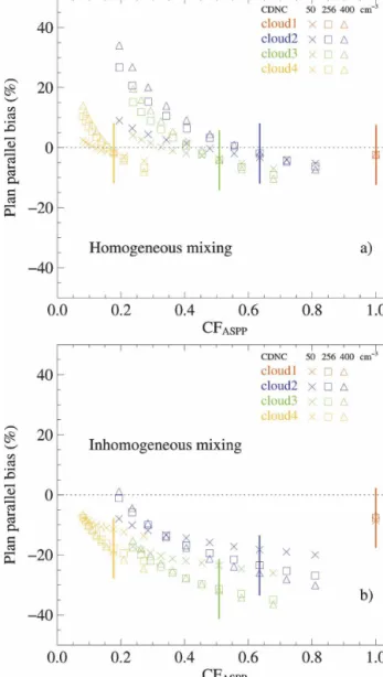
For the estimation of PPM relative biases reported in Table 1, we assume that the GCM cloud parameteriza-tion precisely diagnoses the same LWP and CF as those of the 3D LES simulations. The definition of the cloud fraction however depends on the selected LWP thresh-old. Figure 5 shows the sensitivity of the PPM relative bias to the prescribed cloud fraction, when varying the LWP threshold from 1 to 10 g m⫺2, and using either the homogeneous mixing scheme (Fig. 5a) or the inhomo-geneous one (Fig. 5b). For each scene, the colored ver-tical bar represents the 3D LES CF values of Table 1, which are calculated with an LWP threshold of 3 g m⫺2. For the homogeneous mixing scheme (Fig. 5a), the
PPM relative bias is negative when the LWP threshold is low (from 1 to 3 g m⫺2), as previously reported in the
literature. When the LWP threshold increases, the mean grid LWP is distributed over a smaller cloud frac-tion, the PPM albedo decreases, and positive values of the PPM relative bias are obtained. The figure also shows that there is always a critical CF value, between 3 and 4 g m⫺2, that cancels the PPM bias.
When entrainment mixing is supposed to be of the inhomogeneous type, while the ASPPM is still adiabati-cally stratified, the albedo of the LES scene is signifi-cantly reduced and the PPM relative bias is always negative and stronger (Fig. 5b) irrespective of the LWP threshold used to define the cloud fraction.
TABLE1. Main characteristics of the four simulated cloud fields:
CF, defined with an LWP threshold value of 3 g m⫺2, mean LWP in domain of simulation, and geometrical thickness (H, see text for definition). Also shown are the simulated visible albedo (Avis) and PPM relative bias (PP bias), for three values of initial droplet concentration (Nad), and successively the homogeneous and inho-mogeneous mixing schemes.
Cloud scene CF % LWP g m⫺2 H m Nad cm⫺3 Mixing scheme Avis % PP bias % 1 100 83 310 50 Homogeneous 47 ⫺2 Inhomogeneous 44 ⫺8 256 Homogeneous 65 ⫺2 Inhomogeneous 62 ⫺7 400 Homogeneous 70 ⫺2 Inhomogeneous 67 ⫺6 2 63 8 130 50 Homogeneous 11 ⫺3 Inhomogeneous 9 ⫺18 256 Homogeneous 17 ⫺1 Inhomogeneous 13 ⫺23 400 Homogeneous 20 ⫺1 Inhomogeneous 15 ⫺26 3 50 12 150 50 Homogeneous 11 ⫺3 Inhomogeneous 9 ⫺23 256 Homogeneous 17 ⫺4 Inhomogeneous 12 ⫺31 400 Homogeneous 19 ⫺3 Inhomogeneous 14 ⫺31 4 17 12 230 50 Homogeneous 8 ⫺1 Inhomogeneous 7 ⫺11 256 Homogeneous 10 ⫺1 Inhomogeneous 8 ⫺17 400 Homogeneous 11 ⫺1 Inhomogeneous 9 ⫺19
FIG. 5. PPM relative biases as functions of CF, for 10 values of the LWP threshold, from 1 to 10 g m⫺2, using (a) the homoge-neous mixing scheme and (b) the inhomogehomoge-neous one.
c. Sensitivity of the PPM relative bias to the mixing scheme
At an LWP threshold of 3 g m⫺2for the definition of the cloud fraction, the PPM relative bias is always nega-tive, irrespective of the entrainment-mixing assump-tion, hence the PPM hypothesis systematically overes-timates the mean albedo of a heterogeneous cloud scene. When using a homogeneous mixing scheme, the PPM relative bias varies between ⫺1% and ⫺4%, slightly lower than the ⫺5% estimate of Di Giuseppe and Tompkins (2003), and significantly lower than pre-vious estimates (e.g., Cahalan et al. 1994b; Coley and Jonas 1997). The inhomogeneous mixing hypothesis al-ways produces stronger relative biases, between ⫺6% and ⫺31%. This result attests that the microphysical variability of the droplet size distribution has a stronger impact than the spatial variability of the condensed wa-ter field.
An alternative way of estimating the impact of the mixing process is to proceed inversely. We are now looking for the droplet concentration Npp and liquid
water path LWPppvalues to use in the PPM model to
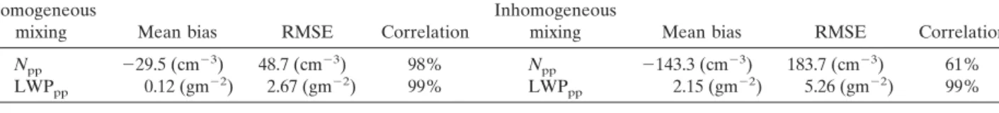
obtain the same cloud albedo as the one of a 3D LES simulation, assuming they both have the same cloud fraction. A series of 1D radiative transfer simulations are performed with SHDOM, for various values of LWP and CDNC, and the resulting albedos at 754 and 1535 nm are stored in a lookup table. The surface al-bedo is set to 0 to reduce ambiguities of the lookup table at low LWP values. Following the method devel-oped by Brenguier et al. (2000), the lookup table is then used to retrieve the CDNC and LWP values that pro-duce the same albedos at both wavelengths, as the LES scene, assuming the cloud fractions of the ASPPM and LES simulations are the same. The CDNC absolute bias is defined asNad⫺Npp, and similarly for the LWP bias.
The results (Table 2) emphasize the impact of the mixing scheme and its preponderance over the LWP variability. For homogeneous mixing, the mean abso-lute bias in CDNC amounts to⫺29.5 cm⫺3, against 0.12
g m⫺2 for LWP. For the inhomogeneous mixing
scheme, the CDNC mean absolute bias is much greater
(⫺143.3 cm⫺3) while the LWP absolute bias remains low (2.15 g m⫺2). Figure 6 shows the comparison be-tween the initial CDNC values of the LES simulation (Nad) and the ones that produce the same albedo in a
PPM calculation (Npp), with the same CF as the LES
one. In the worse case (scene 4, inhomogeneous mixing andNad ⫽400 cm⫺
3
), the CDNC value to use in an equivalent PPM calculation should be of the order of 50 cm⫺3. Note however that this is an extreme case, with a
cloud fraction of 17%, an LWP of 12 g m⫺2 and an
albedo of 9%.
This impact may be important for global simulations of the aerosol indirect effect. GCM models (with a com-bined dynamics and aerosol module), which are pres-ently used to simulate the aerosol indirect effect, rely on a diagnostic of CDNC from the predicted aerosol properties. If we assume this diagnostic is correct, it reflects the initial droplet concentration after activation and before mixing has been active at diluting the initial CDNC. Inhomogeneous mixing, if actually efficient at the top of stratocumulus clouds, may seriously reduce the impact of an aerosol increase, if the initial high
FIG. 6. Initial cloud droplet number concentration (Nad) of the 24 3D simulated cloud scenes vs droplet concentration of the equivalent PPM cloud (Npp), with the same CF as the 3D scene, that produces the same monochromatic albedos (754 and 1535 nm) as the 3D scene.
TABLE2. Statistical comparison between the initial droplet number concentrationNadand mean LWP of the 3D cloud fields and the valuesNppand LWPppto use in PPM calculations to produce the same albedo as the 3D field, assuming the cloud fraction is the same. Statistics are mean absolute bias, root-mean-square error, and correlation factor for the homogeneous (left), and the inhomogeneous mixing scheme (right).
Homogeneous
mixing Mean bias RMSE Correlation
Inhomogeneous
mixing Mean bias RMSE Correlation
Npp ⫺29.5 (cm⫺ 3) 48.7 (cm⫺3) 98% N pp ⫺143.3 (cm⫺ 3) 183.7 (cm⫺3) 61% LWPpp 0.12 (gm⫺ 2) 2.67 (gm⫺2) 99% LWP pp 2.15 (gm⫺ 2) 5.26 (gm⫺2) 99% Fig 6 live 4/C
CDNC value of polluted clouds is further diluted at cloud top.
5. Conclusions
For GCM simulations of the aerosol indirect effect, one has to develop parameterizations that establish a link between the aerosol and its hygroscopic properties, as derived from an aerosol module, on the one hand, and the field of condensed water, as derived from an atmospheric dynamic module. The number concentra-tion of the cloud droplets activated at cloud base that also require an estimate of the mean updraft intensity from the dynamic module is the vector of this relation-ship. The last step is to establish a relationship between the resulting droplet concentration and the vertical pro-file of the droplet size distributions that determine cloud optical properties. This is feasible with the micro-physical model of adiabatic droplet growth, or more sophisticated schemes that account for dilution of the liquid water content by entrainment mixing of drier environmental air.
Entrainment mixing is particularly active at the top of stratocumulus clouds that are exposed to the free tropospheric air from the overlying inversion. This up-per layer is also the region of the cloud that mainly governs its radiative properties. It is not clear, however, if the LWC dilution is accounted for by homogeneous evaporation of all the droplets (constant concentration and decreasing sizes), which is also the most commonly used microphysical scheme in numerical models, or to-tal evaporation of part of them, while the others keep their original size (inhomogeneous mixing with con-stant size and decreasing concentration), which is sug-gested by in situ observations of droplet size distribu-tions.
The tests performed here with realistic cloud scenes reveal that this choice has a strong impact on the de-rived albedo, much stronger than the heterogeneous relative bias that has been extensively discussed in the literature. For fragmented cloud scenes, the PPM al-bedo bias can vary between⫺1% and⫺4% if a homo-geneous mixing scheme is used, while it varies between
⫺6% and ⫺31% with the inhomogeneous mixing scheme. Reciprocally, assuming clouds are correctly pa-rameterized by a GCM, it is possible that an increase in the aerosol concentration may not result in the ex-pected increase of the cloud albedo, if the initial higher droplet concentration of a polluted cloud is further re-duced by inhomogeneous mixing.
In situ measurements suggest that, at the top of stra-tocumulus clouds, mixing is rather of the inhomoge-neous type. However, the comparison between 3D
cal-culations of the cloud radiances at the fine resolution of the LES model scene, and radiances measured from above the cloud layer with multispectral radiometers suggests the opposite.
It is therefore crucial to document more precisely this process and to understand how it may depend upon the intensity of turbulence at cloud top, the generation of negative buoyancy at the inversion level, and the size of the droplets. Considering the discrepancy between in situ measurements and remote sensing of cloud radi-ances, it is also important to find out if the observed inhomogeneous features of mixing in stratocumulus clouds are artifacts of the droplet measurement air-borne technique, so that radiative transfer calculations can be performed with the usual homogeneous mixing scheme, or if they are real and have a significant impact on radiative transfer.
The sensitivity study performed here is limited to monochromatic albedo and a moderate solar zenith angle. This is sufficient to pinpoint the potential impact of entrainment-mixing processes on cloud optical prop-erties, but to conclude on the overall impact of these processes on cloud radiative transfer, additional studies are obviously necessary that shall include their impacts on broadband absorption, transmittance, and albedo for different solar angles.
Acknowledgments.This work has been supported by Météo-France and DGA under Grant 0242127. Anony-mous reviewers are thanked for their careful and con-structive criticism.
REFERENCES
Andrejczuk, M., W. W. Grabowski, S. P. Malinowski, and P. K. Smolarkiewicz, 2006: Numerical simulation of cloud–clear air interfacial mixing: Effects on cloud microphysics.J. Atmos. Sci.,63,3204–3225.
Anger, C. D., S. Mah, and S. K. Babey, 1994: Technological en-hancements to the Compact Airborne Spectrographic Imager (CASI).Proc. First Int. Airborne Remote Sensing Conf. and Exhibition,Strasbourg, France, Environmental Research In-stitute of Michigan, 205–214.
Baker, M., and J. Latham, 1979: The evolution of droplet spectra and the rate of production of embryonic raindrops in small cumulus clouds.J. Atmos. Sci.,36,1612–1615.
——, R. Corbin, and J. Latham, 1980: The influence of entrain-ment on the evolution of cloud droplet spectra.Quart. J. Roy. Meteor. Soc.,106,581–598.
Barker, H. W., 2000: Indirect aerosol forcing by homogeneous and inhomogeneous clouds.J. Climate,13,4042–4049. ——, and J. A. Davies, 1992: Solar radiative fluxes for broken
cloud fields above reflecting surfaces.J. Atmos. Sci.,49,749– 761.
——, and Q. Fu, 2000: Assessment and optimization of the gamma-weighted two-stream approximation.J. Atmos. Sci.,
——, and P. Räisänen, 2004: Neglect by GCMs of subgrid-scale horizontal variations in cloud-droplet effective radius: A di-agnostic radiative analysis.Quart. J. Roy. Meteor. Soc.,130,
1905–1920.
Boers, R., J.-R. Acarreta, and J. Gras, 2006: Satellite monitoring of the first indirect aerosol effect: Retrieval of the droplet concentration of water clouds.J. Geophys. Res.,111,D22208, doi:10.1029/2005JD006838.
Brenguier, J. L., 1991: Parameterization of the condensation pro-cess: A theoretical approach.J. Atmos. Sci.,48,264–282. ——, and W. W. Grabowski, 1993: Cumulus entrainment and
cloud droplet spectra: A numerical model within a two-dimensional dynamical framework.J. Atmos. Sci.,50,120– 136.
——, H. Pawlowska, L. Schüller, R. Preusker, J. Fischer, and Y. Fouquart, 2000: Radiative properties of boundary layer clouds: Droplet effective radius versus number concentra-tion.J. Atmos. Sci.,57,803–821.
——, ——, and ——, 2003: Cloud microphysical and radiative properties for parameterization and satellite monitoring of the indirect effect of aerosol on climate.J. Geophys. Res.,
108,8632, doi:10.1029/2002JD002682.
Breon, F.-M., 1992: Reflectance of broken cloud fields: Simulation and parameterization.J. Atmos. Sci.,49,1221–1232. Burnet, F., and J.-L. Brenguier, 2007: Observational study of the
entrainment-mixing process in warm convective clouds.J. At-mos. Sci.,64,1994–2011.
Cahalan, R. F., 1994: Bounded cascade clouds: Albedo and effec-tive thickness.Nonlinear Processes Geophys.,1,156–176. ——, W. Ridgway, W. J. Wiscombe, Harshvardhan, and S.
Goll-mer, 1994a: Independent pixel and Monte Carlo estimates of stratocumulus albedo.J. Atmos. Sci.,51,3776–3790. ——, ——, ——, T. L. Bell, and J. B. Snider, 1994b: The albedo of
fractal stratocumulus clouds.J. Atmos. Sci.,51,2434–2455. Cairns, B., A. A. Lacis, and B. E. Carlson, 2000: Absorption
within inhomogeneous clouds and its parameterization in general circulation models.J. Atmos. Sci.,57,700–714. Charnock, H., 1955: Wind stress on a water surface.Quart. J. Roy.
Meteor. Soc.,81,639–640.
Coakley, J. A., and T. Kobayashi, 1989: Broken cloud in albedo and surface insolation derived from satellite imagery data.J. Climate,2,721–730.
Coley, P. F., and P. R. Jonas, 1997: The contribution of inhomo-geneities and droplet concentration to the albedo of broken-cloud fields.Quart. J. Roy. Meteor. Soc.,123,1931–1944. Cosma-Averseng, S., C. Flamant, J. Pelon, S. P. Palm, and G. K.
Schwemmer, 2003: The cloudy atmospheric boundary layer over the subtropical South Atlantic Ocean: Airborne– spaceborne lidar observations and numerical simulation.J. Geophys. Res.,108,4220, doi:10.1029/2002JD002368. Cuxart, J., P. Bougeault, and J. L. Redelsperger, 2000: A
turbu-lence scheme allowing for mesoscale and large-eddy simula-tions.Quart. J. Roy. Meteor. Soc.,126,1–30.
Davis, A., A. Marshak, R. Cahalan, and W. Wiscombe, 1997: The Landsat scale break in stratocumulus as a three-dimensional radiative transfer effect: Implication for cloud remote sens-ing.J. Atmos. Sci.,54,241–260.
de Roode, S. R., P. G. Duynkerke, and H. J. J. Jonker, 2004: Large-eddy simulation: How large is large enough?J. Atmos. Sci.,61,403–421.
Di Giuseppe, F., and A. M. Tompkins, 2003: Effect of spatial organization on solar radiative transfer in three-dimensional
idealized stratocumulus cloud fields.J. Atmos. Sci.,60,1774– 1794.
Evans, K. F., 1998: The spherical harmonic discrete ordinate method for three-dimensional atmospheric radiative transfer.
J. Atmos. Sci.,55,429–446.
——, and W. J. Wiscombe, 2004: An algorithm for generating stochastic cloud fields from radar profile statistics.Atmos. Res.,72,263–289.
Feingold, G., R. Boers, B. Stevens, and W. R. Cotton, 1997: A modeling study of the effect of drizzle on cloud optical depth and susceptibility.J. Geophys. Res.,102,13 527–13 534. Guichard, F., and Coauthors, 2004: Modelling the diurnal cycle of
deep precipitating convection over land with cloud-resolving models and single-column models. Quart. J. Roy. Meteor. Soc.,130,3139–3172.
Kobayashi, T., 1993: Effects due on cloud geometry on biases in the albedo derived from radiance measurements.J. Climate,
6,120–128.
Lafore, J. P., and Coauthors, 1998: The Meso-NH Atmospheric Simulation System. Part I: Adiabatic formulation and control simulations.Ann. Geophys.,16,90–109.
Larson, V. L., R. Wood, P. R. Field, J.-C. Golaz, T. H. Vonder Haar, and W. R. Cotton, 2001: Small-scale and mesoscale variability of scalars in cloudy boundary layers: One-dimensional probability density functions.J. Atmos. Sci.,58,
1978–1994.
Latham, J., and R. L. Reed, 1977: Laboratory studies of the effect of mixing on the evolution of cloud droplet spectra.Quart. J. Roy. Meteor. Soc.,103,279–306.
Loeb, N. G., and T. Varnai, 1997: Effects of clouds inhomogene-ities on the solar zenith angle dependence of nadir reflec-tance.J. Geophys. Res.,102,9387–9395.
Marshak, A., A. Davis, P. Wiscombe, and R. Cahalan, 1995: Ra-diative smoothing in fractal clouds.J. Geophys. Res., 100,
26 247–26 261.
——, ——, ——, and ——, 1998: Radiative effects of sub-mean free path liquid water variability in stratiform clouds.J. Geo-phys. Res.,103,19 557–19 567.
Morcrette, J.-J., 1991: Radiation and cloud radiative properties in the ECMWF operational weather forecast model.J. Geo-phys. Res.,96,9121–9132.
O’Hirok, W., and C. Gautier, 1998: A three-dimensional radiative transfer model to investigate the solar radiation within a cloudy atmosphere. Part I: Spatial effects.J. Atmos. Sci.,55,
2162–2179.
Oreopoulos, L., M.-D. Chou, M. Khairoutdinov, H. W. Barker, and R. F. Cahalan, 2004: Performance of Goddard earth ob-serving system GCM column radiation models under hetero-geneous cloud conditions.Atmos. Res.,72,365–382. Pawlowska, H., and J. L. Brenguier, 2000: Microphysical
proper-ties of stratocumulus clouds during ACE-2.Tellus,52B,868– 887.
——, and ——, 2003: An observational study of drizzle formation in stratocumulus clouds for general circulation model (GCM) parameterizations.J. Geophys. Res.,108,8630, doi:10.1029/ 2002JD002679.
Räisänen, P., G. A. Isaac, H. W. Barker, and I. Gultepe, 2003: Solar radiative transfer for stratiform clouds with horizontal variations in liquid-water path and droplet effective radius.
Quart. J. Roy. Meteor. Soc.,129,2135–2149.
Schröder, M., R. Bennartz, L. Schüller, R. Preusker, P. Albert, and J. Fischer, 2002: Generating cloudmask in spatial
high-resolution observations of clouds using texture and radiance information.Int. J. Remote Sens.,23,4247–4261.
Schüller, L., J. Fischer, W. Armbruster, and B. Bartsch, 1997: Calibration of high resolution remote sensing instruments in the visible and near infrared.Adv. Space Res.,19,1325–1334. ——, J.-L. Brenguier, and H. Pawlowska, 2003: Retrieval of mi-crophysical geometrical and radiative properties of marine stratocumulus from remote sensing PACE topical issue.J. Geophys. Res.,108,8631, doi:10.1029/2002JD002680. Sommeria, G., and J. W. Deardorff, 1977: Subgrid scale
conden-sation in models for non precipitating clouds.J. Atmos. Sci.,
34,344–355.
Twomey, S., 1977: The influence of pollution on the shortwave albedo of clouds.J. Atmos. Sci.,34,1149–1152.
Welch, R. M., and B. A. Wielicki, 1989: Reflected fluxes for bro-ken clouds over a Lambertian surface. J. Atmos. Sci., 46,
1384–1395.
Wiscombe, W. J., R. M. Welch, and W. D. Hall, 1984: The effect of very large drops on cloud absorption. Part I: Parcel mod-els.J. Atmos. Sci.,41,1336–1355.