Flow Through an Abrupt Constriction. 2D Hydrodynamic Model Performance and Influence of Spatial Resolution

(1)

Flow Through an Abrupt Constriction

–

2D Hydrodynamic Model Performance

and Influence of Spatial Resolution

Cathie Louise Barton

BE (Civil)

School of Environmental Engineering

Faculty of Environmental Sciences

Griffith University

Submitted in partial fulfillment of the requirements of the Master of

Engineering Science in Environmental Engineering Degree

(2)

SUMMARY I

CATHIE BARTON: FLOW THROUGH AN ABRUPT CONSTRICTION – 2D HYDRODYNAMIC MODEL PERFORMANCE & INFLUENCE OF SPATIAL RESOLUTION

S

UMMARY

This study documents work undertaken to investigate the ability of 2D hydrodynamic models to adequately predict energy losses through an abrupt constriction. In particular, the investigation focuses on the impact that model spatial resolution has on the ability of the model to predict expansion and contraction losses due to the abrupt constriction.

The work outlined in this report began as a result of a perceived lack of understanding in the ability of 2D models to portray the energy losses associated with the turbulent nature of water flow. As flow through an abrupt constriction has been the subject of many investigations throughout the last 50 years, it was decided that such flow would provide a suitable test case for the 2D model assessments.

It was initially decided that a goal standard was needed against which the 2D model predictions could be compared to determine the accuracy of such predictions. Two manual methods using a combination of theoretical and empirical techniques were utilised in the hope that they would provide such a goal standard. In addition, two 1D models were utilised to provide support to the goal standard selected. A suitable goal standard was not found. Ranges of expansion and contraction losses across these four methods were too extreme to allow their use as a standard.

However, the impact of 2D model spatial resolution was still able to be assessed. Two 2D models (TUFLOW and RMA2) were investigated using five spatial resolutions varying from coarse to fine. Flow rates and constriction widths were also varied to provide a comprehensive data set.

Principal outcomes of the study are:

x an improved understanding of different numerical solution schemes;

x an improved understanding of the nature of contracting and expanding flow;

x the confirmation that the spatial resolution of 2D models does have an impact on the ability of these models to predict energy losses due to turbulent effects;

x an understanding of the importance of the eddy viscosity formulation technique on the predictive ability of 2D models;

(3)

CONTENTS II

C

ONTENTS

Summary i

Contents ii

List of Figures vi

List of Tables viii

List of Symbols ix Study Terminology x Statement xi Acknowledgements xii

1 I

NTRODUCTION

1-1

1.1 General 1-1 1.2 Study Objectives 1-2 1.3 Background 1-2 1.3.1 Numerical Models 1-2 1.3.2 Numerical Techniques 1-3

1.4 Flow through an Abrupt Constriction 1-4

1.4.1 General 1-4

1.4.2 Losses 1-4

1.4.3 Flow Regime 1-5

1.4.4 Numerical Modelling 1-5

1.5 Spatial Resolution of 2D Models 1-6

1.5.1 General 1-6

1.5.2 Eddy Viscosity 1-7

2 M

ETHODOLOGY

2-1

2.1 General 2-1

2.2 Test Channel Specifications 2-2

2.3 Calculation Methods Used 2-3

2.3.1 Numerical Models 2-3

2.3.2 Manual Methods 2-3

2.4 2D Model Development 2-3

(4)

CONTENTS III

CATHIE BARTON: FLOW THROUGH AN ABRUPT CONSTRICTION – 2D HYDRODYNAMIC MODEL PERFORMANCE & INFLUENCE OF SPATIAL RESOLUTION 2.4.1.1 TUFLOW 2-4 2.4.1.2 RMA2 2-6

2.4.2 Flows 2-8

2.4.3 Courant Number / Peclet Number 2-9

2.4.4 Eddy Viscosity Formulation 2-11

2.4.4.1 TUFLOW 2-11 2.4.4.2 RMA2 2-11 2.4.5 Processing Results 2-12 2.5 1D Model Development 2-12 2.5.1 MIKE 11 2-12 2.5.2 HEC-RAS 2-13 2.6 Presentation of Results 2-15

2.7 Methodology Comparison with Previous Studies 2-15

3 TUFLOW C

OMPUTATIONS

3-1

3.1 Introduction 3-1 3.2 Computational Procedure 3-1 3.3 Results 3-2 3.3.1 Flow Characteristics 3-2 3.3.2 Losses 3-10 3.4 Discussion 3-25

3.4.1 Effects of Spatial Resolution 3-25

3.4.1.1 Flow Characteristics 3-25 3.4.1.2 Losses 3-25

4 RMA2 C

OMPUTATIONS

4-1

4.1 Introduction 4-1 4.2 Computational Procedure 4-1 4.3 Results 4-2 4.3.1 Flow Characteristics 4-2 4.3.2 Losses 4-9 4.4 Discussion 4-24 4.4.1 Flow Characteristics 4-24 4.4.2 Losses 4-24

5 C

OMPARISON OF

TUFLOW

AND

RMA2 5-1

(5)

CONTENTS IV

5.1.1 Simulation Time 5-2 5.2 Results 5-3

6 MIKE 11 C

OMPUTATIONS

6-1

6.1 Introduction 6-1 6.2 Computational Procedure 6-1 6.2.1 Entrance Loss 6-2 6.2.2 Expansion Loss 6-2 6.2.3 Friction Loss 6-2

6.2.4 Total Head Loss Through Constriction 6-2

6.3 Results 6-3 6.3.1 Sensitivity 6-4 6.4 Discussion 6-5

7 HEC-RAS C

OMPUTATIONS

7-1

7.1 Introduction 7-1 7.2 Computational Procedure 7-1 7.3 Results 7-2 7.3.1 Sensitivity 7-3 7.4 Discussion 7-3

8 M

ANUAL

C

ALCULATIONS

8-1

8.1 Introduction 8-1 8.2 Henderson (1966) 8-1 8.2.1 Expansion Losses 8-1 8.2.2 Contraction Losses 8-2

8.2.3 Dynamic Head Loss Coefficient 8-3

8.2.4 Discussion 8-3

8.3 Waterway Design 8-4

8.3.1 Parameters 8-4

8.3.2 Computation of Backwater 8-5

8.3.3 Contraction and Expansion Losses 8-6

8.3.4 Discussion 8-7

8.4 Other Manual Methods 8-8

(6)

CONTENTS V

10 C

ONCLUSIONS AND

R

ECOMMENDATIONS

10-1

11 R

EFERENCES

11-1

APPENDIX A: F

RICTIONAL

L

OSSES

A-1

APPENDIX B: E

DDY

V

ISCOSITY

B-1

(7)

LIST OF FIGURES VI

L

IST OF

F

IGURES

Figure 1-1 Theoretical Flow Lines Through an Abrupt Constriction 1-4 Figure 2-1 Test Channel Specifications 2-2 Figure 2-2 TUFLOW 15m Grid 2-4 Figure 2-3 TUFLOW 10m Grid 2-4

Figure 2-4 TUFLOW 5m Grid 2-5

Figure 2-5 TUFLOW 2.5m Grid 2-5

Figure 2-6 TUFLOW 1m Grid 2-5

Figure 2-7 RMA Mesh 1 – Coarsest Mesh 2-6 Figure 2-8 RMA Mesh 2 – Coarse Mesh 2-7 Figure 2-9 RMA Mesh 3 – Medium Mesh 2-7 Figure 2-10 RMA Mesh 4 – Fine Mesh 2-7 Figure 2-11 RMA Mesh 5 – Finest Mesh 2-7 Figure 2-12 TUFLOW - Variation of Flows at the Upstream Boundary 2-8 Figure 2-13 RMA2 – Variation in Flows at the Upstream Boundary 2-9 Figure 2-14 Layout of the MIKE 11 Model 2-13 Figure 2-15 MIKE 11 – Variation of Flows at the Upstream Boundary 2-13 Figure 2-16 Layout of the HEC-RAS Model 2-14 Figure 3-1 TUFLOW – Velocities Within the Vena Contracta: b=60m 3-3 Figure 3-2 TUFLOW – Flow Patterns: vc=0.25m/s & b=60m 3-4

Figure 3-3 TUFLOW – Flow Patterns: vc=0.5m/s & b=60m 3-5

Figure 3-4 TUFLOW – Flow Patterns: vc=1m/s & b=60m 3-6

Figure 3-7 TUFLOW – Dynamic Head Loss Coefficients 3-12 Figure 3-8 TUFLOW – Water Levels: vc=0.25m/s (Q=30m3/s & b=60m) 3-13

Figure 3-9 TUFLOW – Water Levels: vc=0.5m/s (Q=60m 3

/s & b=60m) 3-14 Figure 3-10 TUFLOW – Water Levels: vc=0.5m/s (Q=30m

3

/s & b=30m) 3-15 Figure 3-11 TUFLOW – Water Levels: vc=1m/s (Q=120m

3

/s & b=60m) 3-16 Figure 3-12 TUFLOW – Water Levels: vc=1m/s (Q=60m3/s & b=30m) 3-17

Figure 3-13 TUFLOW – Water Levels: vc=1m/s (Q=30m 3

3

/s & b=15m) 3-21 Figure 3-17 TUFLOW – Water Levels: vc=4m/s (Q=480m3/s & b=60m) 3-22

Figure 3-18 TUFLOW – Water Levels: vc=4m/s (Q=240m 3

3

/s & b=15m) 3-24 Figure 4-1 RMA2 – Velocities Within the Vena Contracta: b=60m 4-3

(8)

LIST OF FIGURES VII

Figure 4-2 RMA2 - Flow Patterns: vc=0.25m/s (Q=30m 3

/s & b=60m) 4-4 Figure 4-3 RMA2 - Flow Patterns: vc=0.5m/s (Q=60m

3

/s & b=60m) 4-5 Figure 4-4 RMA2 - Flow Patterns: vc=1m/s (Q=120m3/s & b=60m) 4-6

Figure 4-5 RMA2 - Flow Patterns: vc=2m/s (Q=240m 3

/s & b=60m) 4-7 Figure 4-6 RMA2 - Flow Patterns: vc=4m/s (Q=480m

3

/s & b=60m) 4-8 Figure 4-7 RMA2 - Dynamic Head Loss Coefficients 4-11 Figure 4-8 RMA2 – Water Levels: vc=0.25m/s (Q=30m3/s & b=60m) 4-12

Figure 4-9 RMA2 – Water Levels: vc=0.5m/s (Q=60m3/s & b=60m) 4-13

Figure 4-10 RMA2 – Water Levels: vc=0.5m/s (Q=30m 3

/s & b=30m) 4-14 Figure 4-11 RMA2 – Water Levels: vc=1m/s (Q=120m

3

/s & b=30m) 4-16 Figure 4-13 RMA2 – Water Levels: vc=1m/s (Q=30m3/s & b=15m) 4-17

Figure 4-14 RMA2 – Water Levels: vc=2m/s (Q=240m 3

3

/s & b=60m) 4-21 Figure 4-18 RMA2 – Water Levels: vc=4m/s (Q=240m3/s & b=30m) 4-22

Figure 4-19 RMA2 – Water Levels: vc=4m/s (Q=120m 3

/s & b=15m) 4-23 Figure 5-1 TUFLOW & RMA2 - Dynamic Head Loss Coefficient Envelopes 5-3 Figure 6-1 MIKE 11 - Dynamic Head Loss Coefficients 6-4 Figure 7-1 HEC-RAS - Dynamic Head Loss Coefficients 7-3 Figure 8-1 Plan View of Abrupt Channel Expansion (Henderson, 1966) 8-2 Figure 8-2 Dynamic Head Loss Coefficients (Henderson, 1966) 8-3 Figure 8-3 Backwater Coefficient Base Curves from AUSTROADS (1994) 8-5 Figure 8-4 Dynamic Head Loss Coefficients (AUSTROADS, 1994) 8-7 Figure 9-1 Dynamic Head Loss Coefficients – All Calculation Methods 9-2

(9)

LIST OF TABLES VIII

L

IST OF

T

ABLES

Table 1–1 2D Models Used by Syme et al. (1998) 1-6 Table 1–2 1D Models Used for Comparison by Syme et al. (1998) 1-6 Table 2–1 Test Channel Specifications 2-2 Table 2–2 Details of Models Used 2-3 Table 2–3 Manual Methods Used 2-3 Table 2–4 TUFLOW – Location of Constriction 2-6 Table 2–5 TUFLOW Critical Courant Numbers 2-10 Table 2–6 Summary of Key HEC-RAS Parameters 2-14 Table 3–1 Summary of TUFLOW Simulations Undertaken 3-2 Table 3–2 TUFLOW – Total Head Loss (mm) 3-10 Table 3–3 TUFLOW – Dynamic Head Loss Coefficient Results (vc2/2g) 3-11

Table 4–1 Summary of RMA2 Simulations Undertaken 4-2 Table 4–2 RMA2 - Total Head Loss (mm) 4-9 Table 4–3 RMA2 - Dynamic head loss coefficient Results (vc

2

/2g) 4-10 Table 5–1 Comparison of Computation Points in TUFLOW and RMA2 5-2 Table 5–2 Comparison of Time Factors in TUFLOW and RMA2 5-2 Table 6–1 MIKE 11 – Contraction and Expansion Coefficients 6-3 Table 6–2 MIKE 11 – Total Head Loss (mm) 6-3 Table 6–3 MIKE11 – Dynamic Head Loss Coefficients 6-3 Table 6–4 MIKE 11 Sensitivity Tests 6-4 Table 7–1 HEC-RAS – Total Head Loss (mm) 7-2 Table 7–2 HEC-RAS - Dynamic Head Loss Coefficients 7-2 Table 8–1 Expansion Coefficients (Henderson, 1966) 8-2 Table 8–2 Dynamic Head Loss Coefficients (Henderson, 1966) 8-3 Table 8–3 Waterway Design - Evaluation of Contraction and Expansion Losses 8-6 Table 8–4 Dynamic Head Loss Coefficients (AUSTROADS, 1994) 8-6

(10)

LIST OF SYMBOLS IX

L

IST OF

S

YMBOLS

Symbol Description

a Bottom elevation (m)

Ads Cross-sectional area in channel downstream of constriction (m2)

Aus Cross-sectional area in channel upstream of constriction (m2)

Ac Cross-sectional area in constriction (m2)

D Water depth (m)

Cc Coefficient of Contraction (HEC-RAS)

Ce Coefficient of Expansion (HEC-RAS)

g Acceleration due to gravity (m/s2)

h Water surface elevation = a + D (m)

Lc Length of Expansion Reach (HEC-RAS)

Le Length of Contraction Reach (HEC-RAS)

qs Tributary inflow into system

t Time (usually s)

't Timestep (s)

u Velocity in the x-direction (m/s)

v Velocity in the y-direction (m/s)

vc Average velocity in constriction (m/s)

vus Velocity in the uniform flow area of channel upstream of the constriction (m/s)

vds Velocity in the channel downstream of the constriction where uniform flow has

re-established (m/s)

V Total velocity (m/s)

'x,'y Length of model element in the x and y directions (m) x x

y x x y y y

H

, , , Turbulent eddy coefficients u h

v h :

: , Coriolis forcing in the x and y directions

U

_{Kinematic viscosity (kg/m}3₎

(11)

STUDY TERMINOLOGY X

S

TUDY

T

ERMINOLOGY

Term Units Description

Total Head Loss m Total energy loss across the full length of the study test channel. This includes the expansion loss, the contraction loss and the loss due to friction.

Total Energy Loss m See Total Head Loss

Expansion Loss m Energy loss due to expansion of flow downstream of the constriction. Contraction Loss m Energy loss due to contraction of flow upstream of the constriction.

Total Friction Loss m Energy loss due to frictional effects of the channel bottom across the full length of the study test channel. This is calculated in Appendix A. In this study, the total friction loss is often removed from the total head loss results so that the focus is restricted to expansion and contraction losses (see “Constriction Loss”). Constriction Loss m Energy loss due to losses associated with the contraction and expansion of flow

through the constriction alone. This is equivalent to the total head loss minus the total friction loss.

Dynamic Head m vc2/2g

Dynamic Head Loss Coefficient

- The dynamic head loss coefficient is the sum of the expansion and contraction losses expressed in relation to the dynamic head through the constriction (vc2/2g).

That is, a dynamic head loss coefficient of 1.5 is equivalent to a loss of 1.5 x (vc2/2g); a dynamic head loss coefficient of 0.5 is equivalent to a loss of 0.5 x

(vc2/2g). The dynamic head loss coefficient is dimensionless.

1D Usually referring to a one-dimensional (1D) numerical model. 2D Usually referring to a two-dimensional (2D) numerical model. 3D _{Usually referring to a three-dimensional (3D) numerical model.}

Mesh Network of elements and nodes created when developing a 2D finite element model. The term ‘mesh’ is also sometimes used in this study to refer to the grid of the finite difference model. See also ‘grid’.

Grid Grid of elements and nodes created when developing a 2D finite difference model. For the purposes of this study report, the term ‘grid’ is used solely when referring to a 2D finite difference model network as this network must be uniform throughout. See also ‘mesh’.

Spatial Resolution The spatial resolution of the model is determined by the density of the model network (ie the mesh). The higher the spatial resolution (or ‘mesh resolution’ or ‘grid resolution’), the greater the number of nodes and elements within a defined area. The higher the spatial resolution, the smaller the average element size.

(12)

STATEMENT XI

S

TATEMENT

This work has not previously been submitted for a degree or diploma in any university. To the best of my knowledge and belief, the study report contains no material previously published or written by another person except where due reference is made in the report itself.

(13)

ACKNOWLEDGEMENTS XII

A

CKNOWLEDGEMENTS

The author would like to acknowledge the following people who have provided support and advice throughout this study.

x Chris Nielsen and Mark Jempson for their patience and advice on many occasions;

x Bofu Yu for his support;

x Don Muir for his enthusiasm and help;

(14)

INTRODUCTION

1-1

1 I

NTRODUCTION

1.1 General

Understanding the behaviour of water bodies that surround us is becoming increasingly important as we place more pressure on these natural resources. It is beneficial to be able to quantify the behaviour of water bodies in terms of hydraulics, water quality and other processes in order to predict the impacts of changes to the natural or existing system. Numerical models are often used for this purpose.

The effectiveness of these models in replicating the natural system is dependent upon a variety of factors. These include the quality of physical data used to establish the model, the ability of the modeller to develop a model that is representative of the system, and the numerical capability of the actual model itself in replicating certain aspects of system behaviour. It is on the latter two issues that this study concentrates.

A significant amount of the variability in water quality and other environmental water systems is controlled by the fundamental mechanism of water flow (McCutcheon, 1989). Knowledge of the pathway, volume and velocity of water (hydraulic behaviour) is needed to undertake any fundamental study of water quality or other water process, including modelling investigations (Martin and McCutcheon, 1999). A numerical model used to represent the natural system in a water body must be able to accurately replicate the hydraulic behaviour as well as any other system behaviour, such as water quality. This study focuses on the ability of numerical models to reproduce hydraulic behaviour, specifically the hydraulic behaviour of flow through a constriction. It may be argued that the ability of modelling hydraulic behaviour is critical to the success or otherwise of any numerical modelling of water bodies.

A numerical model which is used to represent the hydraulic behaviour of a water body is called a hydraulic model. Hydraulic models may be broadly categorised into one-dimensional (1D), two-dimensional (2D) and three-two-dimensional (3D) schemes. This study utilises both 1D and 2D numerical models to simulate the flow of water through a constriction. Fully 2D depth averaged solution schemes have been widely used for modelling river and coastal hydraulics and, more recently, have become a practical option for floodplain modelling (Syme et al, 1998). A number of different types of solution schemes are available and are based on the finite difference and finite element methods.

Impacts on hydraulic and water quality behaviour due to such things as developments, point and non-point source discharges, upgrading of road and rail services may be predicted using 1D and 2D numerical models. Results from these assessments often form the critical decision basis upon which design and placement of these works is made. This makes numerical models an integral component of the planning and decision-making process. Thus, the ability of modellers and the models themselves to produce accurate results is important.

This study aims to provide an understanding of the abilities of selected 1D and 2D models to predict flow through a constriction. The focus is on the impact of model spatial resolution on model predictions. A comparison of two 2D schemes (RMA-2 and TUFLOW), two 1D schemes

(15)

(HEC-INTRODUCTION

1-2

CATHIE BARTON: FLOW THROUGH AN ABRUPT CONSTRICTION – 2D HYDRODYNAMIC MODEL PERFORMANCE & INFLUENCE OF SPATIAL RESOLUTION RAS and MIKE-11) and some manual calculations aid in providing an understanding of the behaviour of the different schemes.

1.2 Study

Objectives

The study objectives are as follows:

1. To provide a summary of the numerical solution schemes utilised in this study;

2. To assess the ability of 2D models in predicting energy losses through an abrupt constriction; 3. To assess the impact that the spatial resolution of the 2D models has on prediction of energy

losses through an abrupt constriction.

During the course of the study, with particular regard to Objective 3, it became apparent that further research into the impact of eddy viscosity on model behaviour was needed. This lead to the

development of the additional objective:

4. To provide a preliminary assessment and understanding of the impact of eddy viscosity on 2D model results.

1.3 Background

1.3.1 Numerical Models

Numerical models are developed to represent a natural or existing system. Due to the complexity of the natural environment, numerical models rely on certain simplifying assumptions and theories. The simplification of the complex process creates an uncertainty that is important to recognise and understand.

Hydraulic models specifically, represent hydraulic behaviour of water bodies using a numerical approximation of fluid flow. Due to the complexity of the equations of motion, analytical solutions are not possible. Instead, numerical techniques are used to convert differential equations into algebraic difference forms that can be solved for unknown values at incremental, finite points in space and time. The early models used finite difference numerical techniques. Numerical techniques in use today include finite difference, finite element, finite volume and Langrangian techniques.

The accuracy of the model is related to the degree of complexity represented by the model. Thus, 1D models provide a simpler and less descriptive representation of the real world than 3D models. However, a more complex model is not necessarily a more suitable one, nor does it provide more reliable results. Suitability of a model is determined by the nature of the particular situation being replicated and the accuracy of the output required. For example, assessment of in-bank river flow behaviour may be suitably modelled in 1D and not require a higher dimension model. Alternatively, as discussed by Crowder and Diplas (2000), assessment of suitable fish habitat within a pool and riffle stream may require a 2D or 3D model to reproduce the meso-scale hydraulic behaviour in the downstream shadow of boulders that a 1D model is simply incapable of simulating. In addition, there is a direct relationship between the level of complexity of a model and the amount of data required. If data requirements exceed the data available, the model, despite being complex, cannot reproduce the complexity reliably.

(16)

INTRODUCTION

1-3

CATHIE BARTON: FLOW THROUGH AN ABRUPT CONSTRICTION – 2D HYDRODYNAMIC MODEL PERFORMANCE & INFLUENCE OF SPATIAL RESOLUTION The most common examples of unsteady free surface flow requiring assessment are flows in rivers and tidal flows in estuaries, bays and oceans. 1D schemes are usually used for situations where the flow is channelised or in one direction such as for rivers and estuaries. As truly 1D flow does not occur in nature, the basic assumption involved in undertaking this type of modelling is that channel velocity is uniform over the cross-section and water level across the channel is horizontal. Assumptions such as these date back to the principles proposed by de Saint Venant in 1871 (Cunge et al., 1980). Extensive use of both steady state (flow constant) and hydrodynamic (flow varies with time) 1D models based on these principles has confirmed that the assumptions are adequate for hydraulic modelling in rivers and estuaries.

2D numerical hydrodynamic modelling has its origins in the work of Hansen (1956). Again, truly 2D behaviour does not occur in nature and simplifying assumptions are made. These schemes are normally in plan view with velocities averaged over the depth of the water column.

1.3.2 Numerical Techniques

One of the most common numerical methods is the finite difference method in which time and space are divided into discrete (finite) intervals. Solutions are determined using an explicit or implicit scheme. An explicit scheme expresses one unknown value in terms of several known values. At each time step, a new value can be determined directly (explicitly) using known values from the previous time step. An implicit scheme expresses one unknown value in terms of other unknown values in addition to known values from the previous time step. An implicit scheme requires a matrix solution which means that these schemes require greater computational effort per timestep than explicit schemes.

Explicit schemes are conditionally stable while implicit schemes are unconditionally stable. Stability may be expressed by the Courant number (Abbot, 1979; Syme, 1991, Hardy et al., 1999), which is directly proportional to the timestep. An explicit scheme is only stable for a Courant number of less than or equal to 1. Implicit schemes generally use a Courant number of between 2 and 15 (Syme, 1991) although some studies utilising implicit models (for example, Hardy _{e t a l}., 1999) use Courant numbers of less than 1 to ensure that the simulation quality due to timestep is not an issue when assessing other factors.

Finite element methods assume that the solution has a simple form over small regions (elements). Error-minimising criteria is used to assemble and adjust the individual pieces of the solution so that the best solution over the entire domain is obtained (Martin and McCutcheon, 1999). A system of simultaneous equations is assembled from coefficient matrices for each element. To obtain a solution, these equations are solved simultaneously. The finite element solution technique is often used to represent the water bodies of more-complex shape as the component elements can be assembled in any number of ways.

Finite element models are typically run at much larger timesteps than the finite difference models but require more computational effort per timestep.

(17)

INTRODUCTION

1-4

1.4 Flow through an Abrupt Constriction

1.4.1 General

A constriction in the flow width results in energy dissipation due to turbulence. The dissipation of energy is physically evident by a drop in water level through the constriction. This is usually termed “head loss” and is due primarily to turbulent effects in the contraction of the flow and subsequent expansion of the flow. Constriction types may be of a gradual (tapering) nature or an abrupt nature. Tapered constrictions typically result in lower head losses while abrupt constrictions typically produce larger head losses. Within this study consideration is given only to abrupt constrictions.

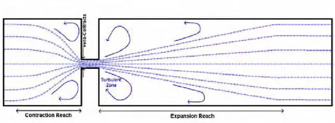
Theoretical flow lines for an abrupt constriction are shown in Figure 1-1. As flow progresses downstream toward a constriction, flow lines converge in the contraction reach to allow flow to pass through the constriction. Within the constriction, the continued convergence of the flow lines can produce a vena contracta, where the active flow width is reduced to less than the constriction width. Divergence of flow occurs downstream of the constriction in the expansion reach where turbulence causes eddies to form.

Figure 1-1 Theoretical Flow Lines Through an Abrupt Constriction 1.4.2 Losses

Studies of turbulent flows through abrupt constrictions using Laser Doppler Velocimetry (El-Sherwey _{e t a l.}, 1996) show that turbulence intensities increase in the contraction reach and increase further within the constriction. However, the highest turbulence intensities occur within the expansion reach. These observations verify the consistent advice given throughout the literature that expansion losses exceed contraction losses for an abrupt constriction (for example, Henderson, 1966; Chow, 1959; Martin and McCutcheon, 1999; HEC, 1998; Formica, 1955)

Total energy loss through a constriction may be divided into three sources: contraction loss, expansion loss and friction loss. It is with the initial two sources that this study is predominately concerned and these have collectively been termed “constriction losses” for the purpose of this study. Terminology used frequently throughout this study report is aimed at distinguishing between these sources. The reader is referred to the Study Terminology summary at the front of this report for clarification on specific terms used.

(18)

INTRODUCTION

1-5

CATHIE BARTON: FLOW THROUGH AN ABRUPT CONSTRICTION – 2D HYDRODYNAMIC MODEL PERFORMANCE & INFLUENCE OF SPATIAL RESOLUTION A simplifying representation of constriction losses may be found in several hydraulics texts (for example, Henderson (1966)), as g v v g v C L o s s E x p a n s io n L o s s n C o n tr a c tio L o s s o n C o n s tr ic ti d s c c c 2 ) ( 2 2 2

Where Cc is a function of the contraction ratio, vc is the average velocity in the constriction

(downstream of the vena contracta), vds is the velocity downstream of the constriction and g is the

acceleration due to gravity. This equation is developed using a combination of empirical and theoretical methods. Within this study, manual calculations such as this are used to provide an indication of the head loss through a constriction for comparison with those constriction losses predicted by numerical modelling. It was intended that these manual calculations, in conjunction with the 1D model results, would provide a goal standard against which the 2D model results could be compared. However, the manual calculations undertaken did not perform as expected. This is discussed in Section 8 and Section 9.

1.4.3 Flow Regime

All calculations undertaken in this study were based on the assumption that the flow regime through the constriction is subcritical. That is, the Froude number

_v _{g y}

is at all times less than 1. As discussed in Section 2.1, this is one of the reasons for limiting the results presented to average constriction velocities of 4m/s and lower.

Supercritical flow occurs when the Froude number exceeds 1. At a velocity of 4m/s and a depth of 2m, the Froude number is around 0.9. An increase in velocity or a decrease in depth will cause the Froude number to increase and may result in the flow regime becoming supercritical. It is important to be mindful of the potential for supercritical flow when assessing model results for the highest average constriction velocities as the numerical models considered are not capable of reliably replicating this flow regime.

1.4.4 Numerical Modelling

1D models, such as HEC-RAS and MIKE 11, use the basic principles in the equation presented above to determine constriction losses. The 1D models use the theoretical/empirical solution method as they are unable to numerically represent the contraction and expansion of flow that causes the energy losses.

2D models may be capable of adequately reproducing these complex flows in a vertically averaged sense. Thus, 2D models do not use the theoretical/empirical solution method of the previous equation but rather rely on the ability of the 2D model to sufficiently represent the flow characteristics that cause energy losses (that is, the contraction and expansion). 2D models may require the use of a combination of theoretical/empirical methods and model equations if the micro complex flow patterns, such as the vena-contracta, are not reproduced.

(19)

INTRODUCTION

1-6

CATHIE BARTON: FLOW THROUGH AN ABRUPT CONSTRICTION – 2D HYDRODYNAMIC MODEL PERFORMANCE & INFLUENCE OF SPATIAL RESOLUTION A comparison of flow behaviour through a constriction for some of the common 2D models currently in use was undertaken by Syme _{e t a l}. (1998). A list of these models and their solution scheme is given in Table 1–1. Syme _{e t a l}. (1998) compared constriction loss results due to flow through an abrupt constriction for each of the models listed to theoretical/empirical calculations and 1D solution scheme results (refer to Table 1–2). Conclusions reached from these comparisons were that a) 2D schemes were able to adequately predict head loss across both a vertical and, possibly a horizontal flow constriction; b) increases in eddy viscosity lead to increases in head losses, and c) time-step variations yielded different results in the MIKE21 model.

Table 1–1 2D Models Used by Syme et al. (1998)

Model Name Solution Technique Solution Scheme Reference

FESWMS Finite Element - FHA

MIKE21 Finite Difference Implicit

(some terms are explicit) DHI (1998)

RMA2 Finite Element - King (1998) TUFLOW Finite Difference Implicit Syme (1991) Table 1–2 1D Models Used for Comparison by Syme et al. (1998)

Model Name Flow Regime Solution

Technique Solution Scheme Reference

MIKE11 Unsteady Finite Difference Implicit DHI (1999) ESTRY Unsteady Finite Difference Explicit WBM (1996)

HEC-RAS Steady - - USACE (1998)

1.5 Spatial Resolution of 2D Models

1.5.1 General

2D models rely on the development of a mesh or grid system to define the model variables such as topography and roughness and to provide a framework upon which the solution schemes operate. In finite element models the typical name for the network defining the model is the mesh, while in finite difference models the typical name used is grid. These naming conventions stem from the fact that a finite difference grid must be a uniform grid of square elements while a finite element mesh can comprise a non-uniform mesh of rectangular and triangular elements with the element size able to change over the model domain. However, this is a typical naming convention rather than standard and the two terms are sometimes used interchangeably. This study uses ‘mesh’ when referring to the finite element model and also when referring to both the finite element and finite difference model, and ‘grid’ is used solely when referring to the finite difference model.

(20)

INTRODUCTION

1-7

CATHIE BARTON: FLOW THROUGH AN ABRUPT CONSTRICTION – 2D HYDRODYNAMIC MODEL PERFORMANCE & INFLUENCE OF SPATIAL RESOLUTION Spatial resolution in 2D models refers to the density, or resolution, of the mesh developed. Selection of the spatial resolution of the model is typically based on a number of factors:

x R e s o lu tio n a n d im p o r ta n c e o f c e r ta in fe a tu r e s w ith in th e to p o g r a p h y. For example, modelling a 10m wide creek entirely within a 2D system requires a mesh resolution of less than 10m. This constraint is particularly applicable to finite difference models which must maintain the same element dimension across the model domain.

x M in im u m m e s h r e s o lu tio n a t w h ic h n u m e r ic a l c o n v e r g e n c e c o u ld b e a c h ie v e d. (Lardner and Song, 1992)

x M a x im u m m e s h r e s o lu tio n th a t a llo w s a s im u la tio n to b e c o m p le te d w ith in a r e a s o n a b le a n d p r a c tic a l tim e fr a m e . For example, a simulation time of 2 weeks is not practical in a real world of budgets and deadlines.

x _{E x p e r ie n c e a n d k n o w le d g e o f th e m o d e lle r .}

A factor not usually included in the selection of a suitable spatial resolution is the effect of model resolution on the solution of the equations. The problems associated with failing to consider this effect are highlighted by many authors who confirm that the spatial resolution of the mesh alone will have an impact on model predictions (Farajalla and Vieux, 1995; Hardy et al., 1999; Crowder and Diplas, 2000, Syme and King (pers. comm. 2000)). Farajalla and Vieux (1995) acknowledge that there is a tendency to assume that an increase in spatial resolution of a model will improve the realism of the model’s predictive ability. Hardy _{e t a l.} (1999) also recognises the trend among many modellers to increase the spatial resolution in a model in the expectation of improved insights into temporal and spatial processes. The following three avenues of thought are responsible for this trend:

x Expected improvements in solution stability as the mesh resolution tends toward the true continuum level;

x The ability of high resolution models to facilitate complex, and thereby more realistic representation of the parameters of the code;

x A closer correspondence between field measurement and model scales.

Hardy _{e t a l.} (1999) believed that mesh resolution is the only unbounded parameter value as there are no accepted standards for mesh construction. This is in contrast to calibration parameters, such as bed roughness, which are bounded and documented in physically realistic ranges (eg Chow, 1959; Henderson, 1966).

The central aim of the study by Hardy _{e t a l.} (1999) was to present an assessment of the impact of spatial resolution on a typical non-linear numerical scheme. The scheme selected was the 2D, implicit, finite element hydraulic model, TELEMAC-2D. Hardy _{e t a l.} (1999) found that mesh resolution effects were at least as important as the Manning’s roughness. Details of these assessments and results are discussed throughout this study report.

1.5.2 Eddy Viscosity

The use of eddy viscosity in 2D numerical modelling provides an approximate representation of the energy losses due to turbulent effects at sub-grid scale (Nielsen, 2000; Rodi, 1980). In assessing the impact of spatial resolution, the current study found that the energy loss results were sensitive to the formulation used to provide the eddy viscosity values. While other studies (eg. Hardy _{e t a l.},

(21)

INTRODUCTION

1-8

CATHIE BARTON: FLOW THROUGH AN ABRUPT CONSTRICTION – 2D HYDRODYNAMIC MODEL PERFORMANCE & INFLUENCE OF SPATIAL RESOLUTION 1999; Crowder and Diplas, 2000) have investigated the impact of varying spatial resolution in 2D models, none of these, with the exception of Nielsen (2000), have investigated the evaluation of the eddy viscosity and the associated impacts.

Although not initially featured as a focus of the current study, the significant impact of the eddy viscosity formulation has meant that it has received considerable attention in these assessments. Appendix B contains a full description of eddy viscosity, evaluation methods and sensitivity assessments.

(22)

METHODOLOGY

2-1

2 M

ETHODOLOGY

2.1 General

Details of the test channel used for all calculation methods throughout this study are presented in Section 2.2. In all methods the test channel is considered to have a constant downstream head level of 2m. The upstream boundary is a discharge boundary and five discharges were used varying from 30m3/s to 480m3/s. Three constriction widths were used: 15m, 30m and 60m. The combination of these variables produced average velocities in the constriction (vc) varying from 0.25m/s to 16m/s.

Supercritical flow is expected to occur within the test channel when average constriction velocities (vc) exceed 4m/s. Supercritical flow may also occur with a vc of 4m/s. As models are typically

incapable of reliably simulating supercritical flow, results from simulations where average constriction velocities exceeded 4m/s were ignored. In addition, although results from simulations where vc is equal to 4m/s have been included, these results should be treated with caution as

supercritical flow may occur and results may not be stable or realistic. Highlighting this is the fact that some methods did not complete simulations at the 4m/s limit due to instabilities. Instabilities at the higher constriction velocities are discussed further throughout this report.

Two 2D hydrodynamic models have been developed to represent the test channel. The 2D models used in this study are RMA2 and TUFLOW. Details are provided in Table 2–2. In order to assess the ability of the 2D models to accurately predict head loss across a constriction in the flow width, other computation techniques are used to compare head loss results. These include development of two 1D models and the use of two theoretical/empirical manual calculation methods. The 1D models used are MIKE11 and HEC-RAS and further details are provided in Table 2–2. Details of the manual calculation methods used are provided in Table 2–3.

Models are used to calculate the total energy loss across the model length. The total energy loss comprises the contraction loss, the expansion loss and the frictional loss. As this study is primarily concerned with expansion and contraction losses through the constriction, frictional losses are calculated manually in Appendix A and are subtracted from the total energy loss to give ‘constriction losses’ (expansion plus contraction losses). A Manning’s ‘n’ of 0.025 has been used to represent the bed roughness in this study. The low value has been chosen to minimise the bed friction effects and ensure that impacts of other parameters, such as the eddy viscosity, are evident.

Constriction losses may be expressed in terms of head with units of metres or as a dimensionless dynamic head loss coefficient (in terms of the dynamic head, vc2/2g). Expressing losses in terms of

the dynamic head allows comparison of constriction losses across all velocities and for this reason this approach has been adopted in this study.

(23)

METHODOLOGY

2-2

2.2 Test

Channel

Specifications

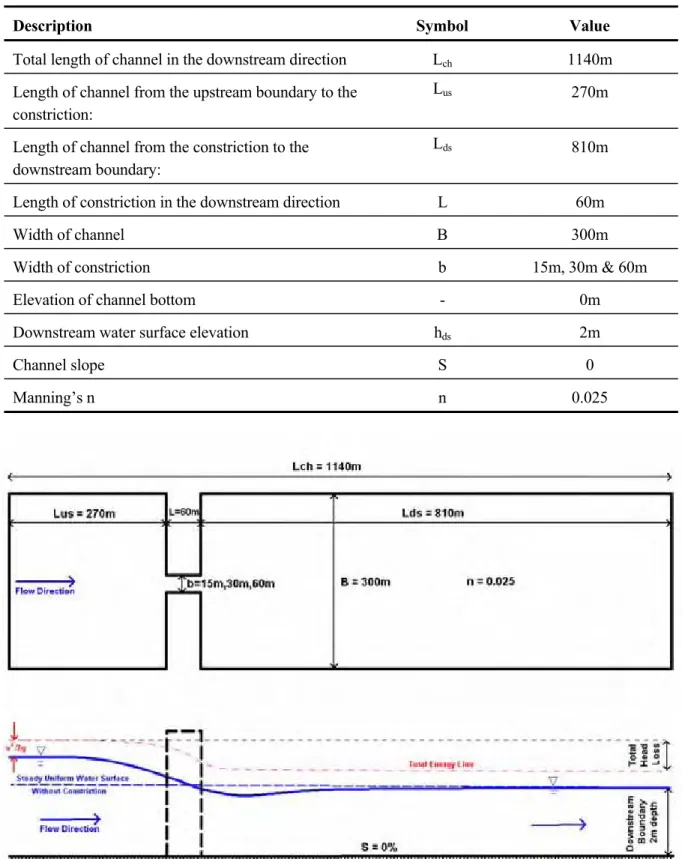
All methods used to calculate head loss in this study use the test channel specifications detailed in Table 2–1 unless otherwise stated.

Table 2–1 Test Channel Specifications

Description Symbol Value

Total length of channel in the downstream direction Lch 1140m

Length of channel from the upstream boundary to the constriction:

Lus 270m

Length of channel from the constriction to the downstream boundary:

Lds 810m

Length of constriction in the downstream direction L 60m

Width of channel B 300m

Width of constriction b 15m, 30m & 60m Elevation of channel bottom - 0m

Downstream water surface elevation hds 2m

Channel slope S 0

Manning’s n n 0.025

(24)

METHODOLOGY

2-3

2.3 Calculation Methods Used

2.3.1 Numerical Models

Details of the models used to determine the total head loss across the model domain are provided in Table 2–2.

Table 2–2 Details of Models Used

Model Name Version Model Type Solution Technique Solution

Scheme Reference

RMA2 6.5 2D Finite Element Implicit King (1998)

TUFLOW 3.0 2D Finite Difference Implicit WBM (2000)

MIKE11 1999b 1D Unsteady Finite Difference Implicit DHI (1992,2000)

HEC-RAS 2.2 1D Steady Standard Step Backwater - HEC (1998)

2.3.2 Manual Methods

A summary of the manual theoretical/empirical methods used to provide a total head loss comparison tool is provided in Table 2–3. Other manual methods were considered for use and are discussed in Section 8.4.

Table 2–3 Manual Methods Used

Method Name Reference Description

“Henderson” Henderson (1966)

Provides a summary of past research into expansion and contraction losses. Combines both empirical and theoretical methods to estimate

expected losses.

Waterway Design

AUSTROADS (1994)

Reproduction of Bradley (1978) for Australian bridge design. Method based on empirical studies involving both laboratory models and field

measurements.

2.4 2D

Model

Development

2.4.1 Spatial Resolution

For each 2D model, five mesh resolutions were developed in order to assess the impact of mesh resolution on constriction loss results. These models were developed according to the test channel specification in Table 2–1 for each width of constriction tested. In conducting these assessments it was found that the eddy viscosity formulation used within the models has a significant impact on the model’s ability to define flow behaviour. Hence, the impact of the eddy viscosity is a major secondary assessment component of this study. Two different eddy viscosity formulations were

(25)

METHODOLOGY

2-4

CATHIE BARTON: FLOW THROUGH AN ABRUPT CONSTRICTION – 2D HYDRODYNAMIC MODEL PERFORMANCE & INFLUENCE OF SPATIAL RESOLUTION tested in each of the 2D models and results are compared. The formulations used are the constant eddy approach and the Smagorinsky formulation. This additional work is presented as Appendix B.

2.4.1.1 TUFLOW

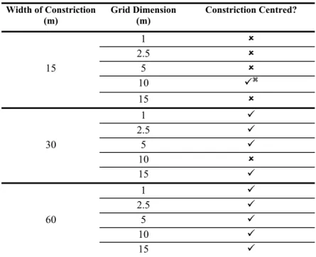
TUFLOW itself was used in conjunction with MapInfo, a GIS based mapping package, to develop the grids that varied in 5 stages of density from coarse (15m Grid) to fine (1m Grid). The differences in grid resolution are demonstrated from Figure 2-2 through Figure 2-6 for the 30m width of constriction subset. In some cases the TUFLOW grid was not able to provide a centred constriction. A summary of constriction placement is provided in Table 2–4. In addition, the 10m grid size was not able to represent the 15m constriction. However, TUFLOW does have the capacity to incorporate a width contraction factor over a number of grid cells (termed the “Flow Constriction” feature in WBM, 2000). By utilising this feature, the 15m width of constriction was modelled as 2 x 10m grid cells with a constriction factor of 0.75.

Figure 2-2 TUFLOW 15m Grid

(26)

METHODOLOGY

2-5

CATHIE BARTON: FLOW THROUGH AN ABRUPT CONSTRICTION – 2D HYDRODYNAMIC MODEL PERFORMANCE & INFLUENCE OF SPATIAL RESOLUTION Figure 2-4 TUFLOW 5m Grid

Figure 2-5 TUFLOW 2.5m Grid

(27)

METHODOLOGY

2-6

CATHIE BARTON: FLOW THROUGH AN ABRUPT CONSTRICTION – 2D HYDRODYNAMIC MODEL PERFORMANCE & INFLUENCE OF SPATIAL RESOLUTION Table 2–4 TUFLOW – Location of Constriction

Width of Constriction (m) Grid Dimension (m) Constriction Centred? 1 8 2.5 8 15 5 8 10 9a 15 8 1 9 2.5 9 30 5 9 10 8 15 9 1 9 2.5 9 60 5 9 10 9 15 9

a_{Flow Constriction Feature used to represent 15m constriction width}

9Constriction Centred in Channel

8Constriction Not Centred in Channel

2.4.1.2 RMA2

The software package SMS 6.0 was used to establish the meshes that varied in density from coarse (Mesh 1) to fine (Mesh 5). The differences in mesh density are demonstrated from Figure 2-7 through Figure 2-11 for the 30m width of constriction subset.

(28)

METHODOLOGY

2-7

CATHIE BARTON: FLOW THROUGH AN ABRUPT CONSTRICTION – 2D HYDRODYNAMIC MODEL PERFORMANCE & INFLUENCE OF SPATIAL RESOLUTION Figure 2-8 RMA Mesh 2 – Coarse Mesh

Figure 2-9 RMA Mesh 3 – Medium Mesh

Figure 2-10 RMA Mesh 4 – Fine Mesh

Figure 2-11 RMA Mesh 5 – Finest Mesh

Difficulties were experienced in developing and assessing these varying mesh densities. The initial approach in developing the mesh was to attempt to automate the mesh generation process as much as possible as this would remove any potential bias in results according to the experience of the modeller. However, meshes generated in this way proved to be extremely unstable and runs could

(29)

METHODOLOGY

2-8

CATHIE BARTON: FLOW THROUGH AN ABRUPT CONSTRICTION – 2D HYDRODYNAMIC MODEL PERFORMANCE & INFLUENCE OF SPATIAL RESOLUTION not be completed. A complete series of new meshes were then created, accounting for the way in which water was expected to flow with increasing localised mesh density in areas where instabilities were believed to be generated. The new series of meshes, which are those shown in the previous figures, were created as they would be by an experienced modeller (advice and guidance received from Nielsen). This changing process was time-consuming but several important conclusions were drawn from the experience and these are detailed in Section 5.

2.4.2 Flows

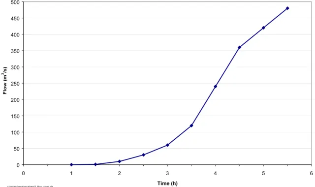
Flows at the upstream boundary over the simulation period were varied from 0m3/s to 480m3/s. Figure 2-12 and Figure 2-13 show the ramping of flows for TUFLOW and RMA2 respectively. The flows at which output is taken are 30m3/s, 60m3/s, 120m3/s, 240m3/s and 480m3/s.

At 4m/s, the flow rate in TUFLOW had to be held constant for an extended period so that the model provided non-fluctuating results (that is, head losses did not fluctuate by more than 2mm). This was particularly relevant for the constriction width of 15m. Thus, all TUFLOW model simulations were run for 8 hours even though some of them required a smaller range of flow rates.

RMA2 simulations were initially ramped to each of the flows for which output was required and then the simulation run at steady state (timestep=0) at each flow to produce a stable result. To increase flows from 240m3/s to 480m3/s it was necessary to ramp the flows through the intermediate flow rates shown in Figure 2-13. Results were not extracted for these intermediate flow rates.

0 50 100 150 200 250 300 350 400 450 500 0 1 2 3 4 5 6 7 8 Time (h) b =15m b = 30m b = 60m c:\project\tuflow\boundaries\report_flow_chart.xls

(30)

METHODOLOGY

2-9

0 50 100 150 200 250 300 350 400 450 500 0 1 2 3 4 5 6 Time (h) c:\project\rma\input\rma2_flow_chart.xls

Figure 2-13 RMA2 – Variation in Flows at the Upstream Boundary 2.4.3 Courant Number / Peclet Number

The Courant Number, Cr, extends from the ‘Courant-Friedrichs-Lewy (CFL) condition’ (Abbot,

1979). The Cr is used for determining a suitable computation timestep for a model simulation. For a

1D scheme the following equation is used to calculate the Courant Number, Cr:

x g D t Cr ' '

For a 2D scheme the following equation applies:

And for a 2D square grid scheme the above equation reduces to:

x g D t Cr ' ' 2

Where: 't = timestep in seconds

'x,'y = length of model element in x and y direction g = acceleration due to gravity (m/s2)

D = depth of water

An implication of the CFL condition is that the stability of an explicit solution scheme is conditional on Cr being less than 1. Both TUFLOW and RMA2 are implicit schemes. Implicit schemes are

(31)

METHODOLOGY

2-10

CATHIE BARTON: FLOW THROUGH AN ABRUPT CONSTRICTION – 2D HYDRODYNAMIC MODEL PERFORMANCE & INFLUENCE OF SPATIAL RESOLUTION However, the inaccuracy (phase error) of an implicit scheme increases with increasing Cr. It is

difficult to determine the magnitude of the inaccuracy except by comparing one simulation with another that used a lower value of Cr. Syme (1991) notes that for most implicit schemes a Courant

Number of between 2 and 15 is typically used.

The value of Cr varies over the model domain as either the element lengths and/or depths vary. The

Courant Number quoted for a particular model is usually the largest over the model domain and is referred to as the critical Courant Number. Courant Numbers for the TUFLOW simulations are presented in Table 2–5. The numbers contained in this table were calculated using the maximum depth predicted by the model for the maximum flow rate (ie 480m3/s) and are thus the critical Courant Numbers. For the majority of the simulation the Courant Numbers will be less than this value. The timesteps were chosen so as to minimise the critical Courant Number.

Table 2–5 TUFLOW Critical Courant Numbers Grid Size (m) Simulation Timestep

(s) Courant Number, Cr 15 7.5 4.0 10 5 6.3 5 4 6.3 2.5 2 4.0 1 0.5 4.0

Sensitivity simulations were undertaken on a subset of the TUFLOW simulation set to determine the impact of a lower simulation timestep (and therefore a lower Courant Number) on results. The differences in total head loss due to timestep reduction were less than 3% of the total head loss. Thus, it may be assumed that the timesteps used in this study provide accurate results.

Hardy _{e t a l.} (1999) removes the need for sensitivity checks of model stability by maintaining a critical Courant Number of less than 1 for all simulations despite TELEMAC-2D being an implicit model. Maintaining a Courant Number of less than 1 across all TUFLOW simulations was not practical as simulation times would have increased by a factor of 4, meaning that the longest simulation would take 16 days to complete (refer to Table 5–2). However, as explained above, sensitivity simulations have confirmed that stability has been achieved with Courant Numbers greater than the limit of 1 used by Hardy _{e t a l.}(1999).

King (1998) recommends consideration of the Peclet number in developing a stable RMA2 simulation. The Peclet number may be used as a guide to mesh density and coefficient selection:

H

U

_V _x P

'

Where:

U

= kinematic viscosity (kg/m3)

'x = mesh spacing (m)

V = velocity along a particular streamline (m/s)

(32)

METHODOLOGY

2-11

CATHIE BARTON: FLOW THROUGH AN ABRUPT CONSTRICTION – 2D HYDRODYNAMIC MODEL PERFORMANCE & INFLUENCE OF SPATIAL RESOLUTION In order for the solution to be stable, the Peclet number should be less than 50. The Peclet number will vary from point to point in a mesh depending on the flow velocity, mesh density and eddy viscosity. The Peclet number can be reduced by increasing the mesh density or increasing the eddy viscosity. (It is interesting to note that when using the Smagorinsky formulation to calculate eddy viscosity (refer to Section 1.5.2 and Appendix B), mesh density is an important variable in the calculation and thus eddy viscosity and mesh density are not able to be independently varied).

The Peclet number has not been calculated in this study as RMA2 does not output the eddy viscosity calculated according to Smagorinsky (refer to Appendix B). Thus, evaluation of the Peclet number is not possible. However, future investigations should consider a means to extract the eddy viscosity from RMA2 to enable calculation of the Peclet number.

2.4.4 Eddy Viscosity Formulation

The use of eddy viscosity in 2D numerical modelling provides an approximate representation of the energy losses due to turbulent effects at sub-grid scale. As this study has found the eddy viscosity to have a significant impact on results, a detailed description and analysis of eddy viscosity is provided in Appendix B. A brief summary is given in this section.

2.4.4.1 TUFLOW

TUFLOW has three methods of determining the eddy viscosity:

x Fixed constant;

x Empirical scaling; and

x Smagorinsky turbulence closure.

WBM (2000) recommends the use of the fixed constant approach when grid size is much greater than the depth. As this was not the case in this study (grid size varies from 1m to 15m and depth varies from 2m to 4m), the Smagorinsky turbulence closure formulation is used. This formulation calculates eddy viscosity values on an element by element basis based primarily on the velocity gradient across the grid, the grid size and an input factor. The factor used in this case is 0.2 which is the same as that used in the RMA2 simulations. There is no minimum limit for the eddy viscosity (that is, the minimum eddy viscosity may be 0).

2.4.4.2 RMA2

RMA2 has three methods of determining the eddy viscosity:

x Fixed constant;

x Scale factor based on size and shape of elements; and

x Smagorinsky turbulence closure.

As the element size typically varies throughout the RMA2 model domain, the standard recommended approach is to utilise the Smagorinksy formulation (King, 1998). This formulation calculates eddy viscosity values on an element by element basis based primarily on the velocity gradient across the grid, the grid size and an input factor. The factor used in this case is the default value of 0.2. In

(33)

METHODOLOGY

2-12

CATHIE BARTON: FLOW THROUGH AN ABRUPT CONSTRICTION – 2D HYDRODYNAMIC MODEL PERFORMANCE & INFLUENCE OF SPATIAL RESOLUTION RMA2, the user has the option of setting a minimum limit to the eddy viscosity. However, in order to remain consistent with TUFLOW, this has been set to 0.

Sensitivity simulations are undertaken for both TUFLOW and RMA2 using the constant eddy viscosity approach with a value of 1m2/s used across the model domain. Substantial differences in results are evident. These are presented and discussed in Appendix B.

2.4.5 Processing Results

TUFLOW and RMA2 provide output in a form able to be imported into the SMS1 package. This allows velocity, head and eddy viscosity results, amongst other output variables, to be contoured and vectored. However, in order to produce the contoured figures contained in this study, a suite of Fortran programs developed by WBM Oceanics Australia were made available to post-process the output data into triangular format. The data for each simulation is then triangulated using the Vertical Mapper (version 2.5) package. Vertical Mapper, in conjunction with MapInfo, is then used to

contour and present the data in the desired format.

1

SMS is a pre- and post-processor for surface water modelling, analysis, and design developed by Brigham Young University. While it includes two-dimensional finite element, two-dimensional finite difference, three-dimensional finite element and one-dimensional backwater modelling tools, it has been used in the current study to prepare RMA2 grids and post-process 2D model results only.

2.5 1D

Model

Development

The 1D MIKE 11 and HEC-RAS models are used to calculate losses through the abrupt constriction for comparison with the two-dimensional model computations.

2.5.1 MIKE 11

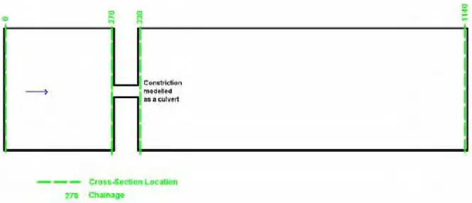
In MIKE 11 the constriction is modelled as one rectangular culvert of open section type with a length in the flow direction of 60m. The top of the culvert is set at a height above the maximum water level and does not influence computations. All coefficients used are the MIKE 11 default coefficients (DHI, 2000). Dx-max (the maximum distance between cross-sections before automatic interpolation of a h-point occurs) has been set at a value greater than the overall channel length. This was done to ensure that the results were produced with the exact model layout shown in Figure 2-14.

The Courant number is given by the following equation:

x g D v t Cr ' '

Where: 't = timestep in seconds

'x = minimum distance between cross-sections g = acceleration due to gravity (m/s2)

D = depth of water

v = velocity

A timestep of 2 minutes has been used for all MIKE 11 simulations. This gives a critical Courant number of 0.3 which is much less than the maximum of 10 specified by DHI (2000) and thus the model simulations satisfy the Courant stability criteria.

(34)

METHODOLOGY

2-13

CATHIE BARTON: FLOW THROUGH AN ABRUPT CONSTRICTION – 2D HYDRODYNAMIC MODEL PERFORMANCE & INFLUENCE OF SPATIAL RESOLUTION Figure 2-14 Layout of the MIKE 11 Model

0 50 100 150 200 250 300 350 400 450 500 0 1 2 3 4 5 6 7 8 9 Time (h)

Figure 2-15 MIKE 11 – Variation of Flows at the Upstream Boundary 2.5.2 HEC-RAS

In HEC-RAS the abrupt constriction is modelled as a bridge opening with no piers. The deck is set at a level above the maximum water surface elevation so that it does not influence computations. Ineffective flow areas are defined according to the manual (HEC, 1998). The method of calculating friction slope is the default method using the average conveyance equation. Physical characteristics of the channel are as specified in Table 2–1. The model layout is shown schematically in Figure 2-16.

(35)

METHODOLOGY

2-14

CATHIE BARTON: FLOW THROUGH AN ABRUPT CONSTRICTION – 2D HYDRODYNAMIC MODEL PERFORMANCE & INFLUENCE OF SPATIAL RESOLUTION Key issues associated with the development of the HEC-RAS model for this study are as follows:

x Selection of expansion and contraction coefficients, and

x Selection of the expansion and contraction reach lengths.

The methods and calculations used in these selection processes are covered in detail in Appendix C. A summary of the values selected for each of the key parameters is provided in Table 2–6.

Figure 2-16 Layout of the HEC-RAS Model

Table 2–6 Summary of Key HEC-RAS Parameters

b Q Expansion Reach Contraction Reach

(m) (m3/s) Le Ce Lc Cc 30 570 0.8 330 0.5 15 60 570 0.8 330 0.5 120 570 0.8 330 0.5 30 540 0.7 310 0.5 60 540 0.7 310 0.5 30 120 540 0.7 310 0.5 240 540 0.7 310 0.5 30 360 0.4 170 0.4 60 360 0.4 170 0.4 60 120 360 0.4 170 0.4 240 360 0.4 170 0.4 480 360 0.4 170 0.4

(36)

METHODOLOGY

2-15

2.6 Presentation

of

Results

For each calculation method, total head loss results are presented in units of millimetres. Constriction losses (total head loss minus friction loss) are then presented as a dynamic head loss coefficient. As explained in the study terminology section, a dynamic head loss coefficient of 1.5 is equivalent to a constriction loss of 1.5 x (vc2/2g) where vc is the average velocity through the constriction. It is

important to note that there are advantages and disadvantages in using vc as the basis for the dynamic

head:

Advantages:

x vc is simple to calculate. vc = Q/Ac where Ac is the average constriction area.

x vc remains constant regardless of model spatial resolution or method of calculation used.

Disadvantages:

x vc does not account for the presence or otherwise of the vena contracta.

x vc is neither the maximum or minimum velocity through the constriction.

x At low values of vc, total head loss is also low and dynamic head loss coefficients are very

sensitive to the dynamic head (vc2/2g). The accuracy of the dynamic head calculated using vc at

these low velocities may introduce sensitivity errors into the coefficients. This is discussed further throughout the report.

2.7 Methodology

Comparison with Previous Studies

This current study provides some extension of the previous work by Syme _{e t a l.} (1998) described in Section 1.3.2. Head losses for varying widths of constriction for varying flows are calculated using two 2D models, two 1D models and theoretical/empirical manual calculations. However, the specific focus of this study is the impact that varying the spatial resolution of the 2D models has on flow behaviour. Five sets of meshes were developed for each 2D model ranging from coarse to fine resolution. It is similar to the work undertaken by Hardy _{e t a l.}(1999) who investigated the impact of mesh resolution across 7 different mesh resolutions for one 2D model. However, there are several significant differences between this current study and that undertaken by Hardy _{e t a l.}(1999) that are important to note:

x Hardy _{e t a l.} (1999) investigated a compound meandering channel rather than a simple rectangular channel.

x Increasing the model spatial resolution by Hardy _{e t a l.} (1999), resulted in a change to the channel dimensions due to the means employed to define the topography. Therefore, prior to any impact that may have been generated by the difference in the solution of equations due to the changing resolution, the actual channel volume and conveyance was different. No scaling corrections were made as Hardy _{e t a l.}(1999) believes that the differences in the filtering of data is one of the first effects of spatial resolution. While this is true, the resolution of important topographical features is one of the key factors in selecting an appropriate mesh resolution. Therefore, if the modeller believes that this factor is satisfied by the mesh resolution chosen, it is necessary to investigate the impacts that occur beyond this resolution if the mesh is further refined. The current study avoids this complication as all meshes developed define the same simple,