Detecting Path Anomalies in Time Series Data on Networks

Detecting Path Anomalies in Time Series Data on Networks

Timothy LaRock

Network Science Institute Northeastern University

Boston, MA, USA

Vahan Nanumyan

Chair of Systems Design ETH Zürich Zürich, Switzerland

Tina Eliassi-Rad

Network Science Institute Northeastern University

Boston, MA, USA

Ingo Scholtes

Data Analytics Group University of Zurich

Zürich, Switzerland

Giona Casiraghi

Chair of Systems Design ETH Zürich Zürich, Switzerland

Frank Schweitzer

Chair of Systems Design ETH Zürich Zürich, Switzerland

ABSTRACT

The unsupervised detection of anomalies in time series data has important applications, e.g., in user behavioural modelling, fraud detection, and cybersecurity. Anomaly detection has been exten-sively studied in categorical sequences. But we often have access to time series data that containpathsin networks. Examples include transaction sequences in financial networks, click streams of users in networks of cross-referenced documents, or travel itineraries in transportation networks. To reliably detect anomalies we must ac-count for the fact that such data contain a large number of indepen-dent observations of short paths constrained by a graph topology. Moreover, the heterogeneity of real systems rules out frequency-based anomaly detection techniques, which do not account for highly skewed edge and degree statistics. To address this problem we introduce HYPA, a novel framework for the unsupervised de-tection of anomalies in large corpora of variable-length temporal paths in a graph. HYPA provides an efficient analytical method to detect paths with anomalous frequencies that result from nodes being traversed in unexpected chronological order.

1

INTRODUCTION

Anomaly detection refers to the problem of finding “patterns in data that do not conform to a well defined notion of normal behaviour,” [16]. The importance of anomaly detection techniques rests on the fact that such anomalous patterns may carry important meaning. Examples include anomalous usage or traffic patterns used to detect cyberattacks, anomalous sensor readings that may identify immi-nent faults in technical systems, or anomalous transactions patterns used to detect fraud and compliance violations in financial systems. In order to assess which data represent “anomalies”, we must de-fine what we consider “normal behaviour” in the particular system under study. Given this baseline of “normal behaviour”, we must develop methods to efficiently assess which instances in the data exhibit deviations from this baseline. Lastly, we need techniques to argue which of those observed deviations aresignificantgiven the fluctuations and randomness contained in data.

While the anomaly detection problem has been studied exten-sively for general categorical sequence data, we are often confronted with time series data capturingpaths through networks. Such data have special characteristics. Different from general categorical se-quences, an underlying graph topology constrains which paths, i.e., sequences of node traversals, can possibly occur. Moreover, the

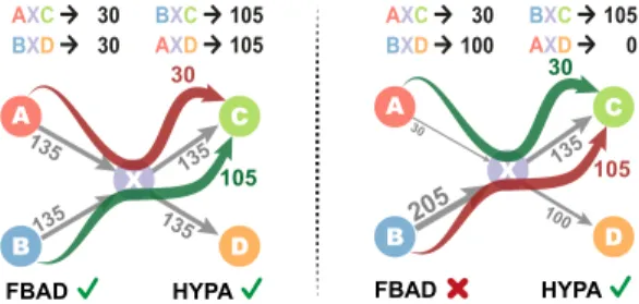
graphs in which paths are observed often exhibit strong geneities, e.g., heavily skewed node degree distributions or hetero-geneous edge statistics. These heterogeneities invalidate frequency-based anomaly detection techniques that do not account for the fact that in real systems some paths are more likely to be observed at random than others (see example in Fig. 1).

135 C D A B X C D A B X FBAD 135 135 135 30 135 205 100 30 105 30 105 AXD 105 BXC 105 BXD 30 AXC 30 AXD 0 BXC 105 BXD 100 AXC 30

HYPA FBAD HYPA

Figure 1: Frequency-based anomaly detection (FBAD) can be used to identify ground truth under- (red) and over-represented (green) paths in graph with homogenous edge statistics (left), but fails to identify anomalies in data with heterogeneous edge statistics (right). Our proposed method HYPA succeeds in both scenarios. For illustrative purposes, the example only contains paths of lengthk=2, while HYPA detects anomalies at any lengthkin variable-length data.

Closing this gap, we consider the problem of detectinganomalous pathsin heterogeneous graphs based on large time series data capturing sequences of node traversals. Our definition ofanomalous pathsis based on a memoryless baseline model, which assumes that the chronological order of node traversals is uniquely determined by the graph topology and the statistics of edge traversals. Our method, HYPA thus detects anomalous paths consisting of nodes with unexpected temporal traversal patterns.

This problem is of practical relevance in a number of scenar-ios. For a graph capturing hyperlinks between web pages, we can consider a set of click streams generated by users navigating the pages. Here, anomalous paths between Web pages could translate to semantic similarities or differences that lead users to navigate links in this specific order more or less often than expected at random. Similarly, for data containing sequences of transactions between actors in a financial network, path anomalies signify frequent paths of money exchange across subsets of financial actors. And for trajec-tories of passengers on flights through the network of US airports,

anomalous paths convey information about the role of airports in routing flights through the country.

To support such studies we propose HYPA , a novel method for unsupervised anomaly detection in collections of variable-length sequences capturing paths in a graph. Our main contributions are: (i) We introduce the problem of detectingpath anomalies, referring to paths in a graph that occur more or less often than expected under a random null model. We further show that the problem of detectinganomalous pathsof lengthkcan be reduced to the problem of detectinganomalous edgesin ak-dimensional De Bruijn graph model of paths in a graph.

(ii) We use an analytically tractable statistical model of random, weighted De Bruijn graphs to derive closed-form expressions for the cumulative weight distribution of paths of any lengthk observed in data. We introduce HYPA, a path anomaly detection algorithm that leverages these weight distributions to detect paths that occur significantly more or less often than expected at random. Anomalies are identified based on a discrimination threshold, which can be set either heuristically or according to ap-value of a hypothesis test.

(iii) We validate HYPA in synthetic data with known anomalies introduced for different path lengths. The results show that HYPA detects anomalies at the correct orderkwith high ac-curacy. The applications of HYPA to empirical data on user trajectories in transportation and information systems show that the detected anomalies can be validated using geographical or semantic information.

Providing a novel scalable method for the unsupervised detec-tion of anomalies that is grounded in graph theory and statistical modeling, our work opens new opportunities for the mining of patterns in time series data on networks. The runtime of HYPA scales linearly with the size of the data, making it suitable for big data scenarios.

2

RELATED WORK AND BACKGROUND

Before introducing our method, we first summarize related works on anomaly detection and sequential pattern mining. We further provide the background of higher-order graph models and statistical graph ensembles underlying our method.

2.1

Related Work

Considering the large body of research on anomaly detection in time series data [24], and keeping in mind the focus of this paper, we limit our review to related works on (i) anomaly detection in discrete sequences, (ii) sequential pattern mining, and (iii) graph-based anomaly detection. Since we are concerned with the unsupervised detection of path anomalies we further exclude (semi-)supervised and reinforcement learning techniques.

Anomaly Detection in Sequence Data.Following [17, 18], anom-aly detection techniques for discrete sequences fall into different categories that address fundamentally different application sce-narios. Sequence-based anomaly detection assumes that we are given a setS={s1,s2, . . . ,sn}of sequencessi =(xj)j=1, ...,l_i over a discrete alphabetΣ, possibly with variable lengthsl_i. One then considers the problem of finding anomalous instancess_i inS, e.g., by assigning an anomaly score to each sequence in the database.

For instance, if the sequencess_icapture sensor readings of different machines or system call sequences in user sessions on a computer, these anomalies can tell us which machines are likely to experience imminent failures or which user accounts have likely been hijacked by an intruder. Different approaches have been used to establish a random baseline against which sequences are defined as “anoma-lous”. Some works use (hidden) Markov chain models, e.g., to detect (groups of ) sequences which show significant differences in terms of state transition probabilities [4, 29, 31, 45]. Other methods use nearest-neighbours algorithms [32] or distance measures [47] to quantify how any given sequences_jdiffers from other instances in

S. Adopting a collective definition of anomalies [16], a third class of methods is based on hypothesis testing techniques to detect outliers in the distribution of features of sequences [5, 30, 46].

Sequential pattern mining.A common feature of the works above is that they focus on anomalies at the level of a whole sequences_i withinS. Addressing a different problem , a number of works instead consider the problem of finding anomalouspatternsorsubsequences within a long sequenceS=(x_i)_i=

1, ...,n[17]. This is closely related

to sequential pattern mining [1], e.g., algorithms to quickly find the most frequent subsequences in large sequence data [20, 43]. Other works address this problem based on statistical methods, e.g., using Markov modelling techniques [12, 25, 37, 39, 50, 53], hypothesis testing [8, 44], or information-theoretic methods to detect “surpris-ing” subsequences [9, 15, 27]. Applications include the detection of common patterns in user trajectories [38, 50], testing hypothe-ses about generative proceshypothe-ses of trajectory data [44], or finding clusters in click streams and other sequence data [12, 37].

Temporal Anomaly Detection in Graphs.Compared to the problem of anomaly detection in general discrete sequences addressed in the works above, the problem motivating our method is different in multiple ways. First and foremost, the methods above make no as-sumptions about the relational structure of data, while we consider sequential data capturing paths in a (weighted and directed) graph topology. This aligns our work more closely to anomaly detection techniques for temporal graph data that have been developed in the graph mining community [3, 35]. As summarized in [3, 10] these works mainly study the detection of change events [2] or cluster structures in evolving graphs [11, 37]. Different from these prob-lems, our method uses a setSof sequences – capturing, e.g., click streams in a hyperlink graph, humans travelling in a transporta-tion network, or communicatransporta-tion sequences in a social network – to identify paths of nodes that are traversed more or less often than expected. Hence, rather than making statements about anoma-lous instances inS, we use collective statistical information inSto identify sequences of nodes traversed withanomalous frequencies.

2.2

Background

Due to the growing volume of time series data capturingtrajectories orpathsin networked systems, the modeling of patterns in these data has become the focus of recent works in graph mining and net-work science. Addressing the detection of exceptional trajectories, previous work [4, 6] develops a framework that can be used to test hypotheses about generative processes. A number of recent works use higher-, variable-, and multi-order models of paths in order to detect, model and quantify deviations from the Markovian expecta-tion [28, 36, 38, 40–42, 52]. Contributing to this line of research, our

HYPA

graph G path anomalies

HYPA scores +12.57 -12.57 +11.69 -11.69 AXD BXC BXD AXC k=2 k=3 k=4 CDF of path counts Pr(X ≤x) 1 100 200 0 A X C B X D A X D B X C 1 2 3 4 5 6 7 8... AX BX XC XD 0 50 100 150 200 250 30 100 135 205 edge counts AXC AXD BXC BXD 0 20 40 60 80 100 120 30 105 100

path counts _{randomised paths}deviations from

AX XC XD 100 BX 30 105 0 validation k-th order De Bruijn graph distribution functions of path counts C D A B X _paths HYP A score

fraction of randomised paths AXD BBXXCD AXC

robustness against noise

(a) (b) (c) (d)

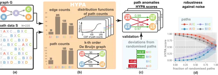
Figure 2: A toy example of path dataSobserved in a graphGillustrates path anomaly detection with HYPA (focusing on k=2). Given a set of sequences traversing nodesA,B,X,C, andDin a graph (a), HYPA uses higher-order De Bruijn graphs to derive closed-form expressions for the cumulative distribution function of all possible paths in the graph (b). HYPA computes HYPA-scores (c) that allow reliable detection of over- and under-represented paths, even in situations where the least frequent path (AXC) is over-represented, while the most frequent path (BXC) is under-represented. Progressive randomization of the data gradually levels HYPA-scores (d), translating to a decreasing confidence at which we detect path anomalies.

work provides a new foundation for the efficient detection of path anomalies in time series data on graphs. Our method specifically overcomes complications in the reliable detection of significant path anomalies in directed and weighted graphs, which (i) have not been addressed in the graph mining and sequence mining literature, and (ii) rule out applications of common frequency-based methods to detect collective anomalies.

Contributing to recent research on higher-order graph mod-els [28], our method is based on a projection that reduces the prob-lem of detecting anomalouspathsin a (first-order) graph model to the problem of detecting anomalousedgesinhigher-ordergraph models that resemble De Bruijn graphs [19]. Similar to [41], we define a higher-order De Bruijn graph model of paths as follows:

Definition 2.1 (k-th order De Bruijn graph model of paths). For a given graphG=(V,E)andk∈_Nwe define ak-th order De Bruijn graph of paths inGas a graphGk=(Vk,Ek), where (i) each node#”v :=v# ”₀v₁. . .v_k−1∈Vkis a path of length1k−1 inG, and (ii)(#”v,w#”) ∈Ekiffvi+1=wifori=0, . . . ,k−2.

This definition has several implications. First, any two nodes#”v andw#”connected by an edge in ak-th order graphGkrepresent two paths of lengthk−1 that overlap in exactlyk−1 out ofk nodes. Since paths in a graph are transitive, each edge(v#”,w#”)in Gkrepresents a path of lengthkin graphG. This implies that the graphGitself is a first-order De Bruijn graph of paths of length one (i.e., edges) inGi.e.,G1 =G. We can see De Bruijn graphs as generalization of standard, first-order graphs to higher-order models of paths of lengthk, where any path of lengthqinGk translates to a path of lengthk+q−1 inG. We iteratively construct such De Bruijn graph models of orderkby means of a line graph transformation of the De Bruijn graph model of orderk−1.

1

We assume that path length counts the number of edges traversed inG

The benefit of this representation is that it allows us to represent the frequencies of paths of lengthkobserved in a graph to the weights of edges in ak-th order De Bruijn graph. This can be seen in the illustration of a De Bruijn graph with orderk=2 in Fig. 2, where nodes represent paths of lengthk−1=1 (i.e., edges inG) that overlap ink−1=1 nodes, while edges represent all paths of lengthk=2. Note that we also consider allsubpaths of length two, i.e., paths of length two contained in longer paths.

This simple higher-dimensional projection of paths in a graph allows us to reduce the problem of detecting paths of lengthkthat exhibit anomalous frequencies to the problem of detecting anoma-lous edge weights in ak-th order De Bruijn graph. To understand which edge weights exhibit “anomalies”, we need a suitable null model that provides the baseline against which we want to com-pare the observed weights. We specifically need a way to generate randomized configurations of the path data that selectively destroy those patterns that we are interested in, while preserving all other characteristics. Thanks to the projection of paths to edges of a di-rected and weighted (De Bruijn) graph, we can address this problem by employingstatistical graph ensembles, which randomize certain aspects of a graph (i.e., the weights of edges or the topology) while preserving other characteristics. Examples include simple models that randomize the topology of a given graph while preserving the (expected) number of edges [23], as well as combinatorial models that preserve the degrees of nodes [34].

An analytically tractable formulation of such a model for directed and weighted graphs was recently proposed in [13]. It treats the random generation of weighted graphs as an urn problem, where random edges are drawn without replacement from a population of multi-edges connecting different pairs of nodes. Through this for-mulation, the probability of generating edges with specific weights can be calculated based on the multivariate hypergeometric distri-bution. While this formulation can be used to detect anomalous edges in social networks [14], no analytically tractable null models

that account for the special characteristics of De Bruijn graphs, i.e., the fact that a directed edge between two nodes in ak-th order De Bruijn graph can only exist if the corresponding path exists in the underlying graph, have been proposed. Closing this gap, we present a novel method to detect path anomalies based on statistical ensembles ofk-th order De Bruijn graph models.

3

HIGHER-ORDER HYPER-GEOMETRIC

PATH ANOMALY DETECTION

We now define the problem ofpath anomaly detection, illustrate the problem in an example, and introduce our proposed solution.

Definition 3.1 (Path Anomaly Detection). LetG =(V,E)be a directed graph andSa set ofnsequencess_i, where each se-quences_i =v0v1. . .vl_i is apathof lengthliinG, i.e.vj ∈V for j∈ [0, . . . ,l_i]and(v_j,v_j+1) ∈Eforj ∈ [0, . . . ,li −1]. Fork>1, identify all paths#”p =v# ”0. . .vkof lengthkinGwhose frequencies, as subpaths, inSsignificantly deviate from the frequencies expected in a(k−1)-order model of pathsinG.

We do not assume that the observed sequences have the same lengthsl_i and we particularly consider data capturing many short paths. Unlikesequence-based anomaly detection techniques[17], we are not interested in assigning ananomaly scoreto each sequence si inS. We instead want to use the instances inSto identify which paths in the graph exhibit anomalous frequencies compared to a “random baseline”. Hence, rather than detecting anomalies inS, we useSto learn which paths inGare traversed in an anomalous fashion. To complete our definition ofanomalies, we define a gen-erativenull modelfor paths that builds on definition 2.1. We use it to establish the baseline against which we detect anomalies [16].

Definition 3.2 (k-th order model of paths). For a graphGlet Gk _=(Vk_,Ek₎be ak-th order De Bruijn graph of paths inG(cf. Def. 2.1). For each edgee :=(v# ”0. . .vk−1,v# ”1. . .vk) ∈ Ek let the weightf(e)be the frequency of subpathv# ”₀. . .v_kinS. LetTkbe the transition matrix of an edge-weighted random walk onGk, i.e.,Tk_#” vw#” := f( #” v,w#”) Í #” x∈V kf(#”v,#”x)

. For a path #”p = v# ”₀v₁. . .v_l with l ≥k thek-th order model of pathsgenerates #”p with probabil-ityÎl

i=kTkv# ”i−k...vi−1v# ”i−k+1...vi.

The model defined above generates paths of lengthlby perform-ingl−k+1 random walk steps in ak-th order De Bruijn graph. We can use such a model to generate random paths of lengthl≥k that respect (i) the topology of the underlying graphG, and (ii) the frequencies of paths of lengthkobserved inS.

Our definition of path anomalies of lengthkis based on a null model of orderk−1. Fork=2, the null model of order(k−1)=1 is simply an edge-weighted random walk on the graphG. In this case, the sequence of nodes traversed by paths isMarkovian, i.e., the nodev_i+1on a path only depends on the current nodevi and the graph topology. Apart from the topology, the model accounts for the frequencies at which paths inStraverse edges inG. That is, if an edge(b,c)is traversed more often than(b,d)we expect pathabc# ”to occur more often thanabd# ”. Fork>2, the null model corresponds to an edge-weighted random walk on a De Bruijn graph of order(k−1)>1, where weighted edges capture the frequencies of subpaths of lengthk−1 inS. This approach to generating a null

model is key to disentangling path anomalies that unfold at different lengthsk:For any given lengthkit enables us to exclusively detect those path anomalies that do not trivially result from anomalous path frequencies at shorter lengths.In other words, to answer the question whether aspecificpathabcd# ”of lengthk=3 is observed more or less often than expected, we discount for any anomalies of shorter pathsabc# ”andbcd# ”contained inabcd# ”.

3.1

Illustrative Example

A simple example to illustrate the path anomaly detection problem fork = 2 is shown in Fig. 2, which gives a high level overview of our method HYPA. Limiting our focus to paths that traverse nodesA,B,X,C, andD, we consider a setSthat contains 235 (sub)paths of length two. We observe strong heterogeneities in the path frequencies, where the most frequent pathBXC# ”occurs 105 times, while the least frequent pathAXC# ”occurs only 30 times.

Assume we want to detect for which paths of lengthk=2 the frequencies deviate from the expectation in a first-order null model. If all paths were expected to occur with the same frequency, we could directly answer this question based on the distribution of path frequencies (cf. Fig. 1). Such an approach would trivially detect that pathAXC# ”occurs more often than expected while pathBXC# ” occurs less often than expected. However, the edge frequencies in our toy example show strong heterogeneities, where, for example, edge(B,X)is traversed about seven times more often than edge

(A,X)(see Fig. 2). If we account for this heterogeneity of edges (i.e., paths of lengthk−1=1), the question of which paths of length k=2 exhibit statistically significant deviations becomes non-trivial. In particular, the same observed frequencyf can be (i) “normal”, i.e., expected, for one pathp#”₁, (ii) a significant over-representation for anotherp#”2, and (iii) an under-representation for a thirdp#”3.

We could address this problem by simulating the first-order model: we can randomly generate paths by means of a random walk model and then count their average frequencies across many simulations. A comparison of observed vs. average frequencies of paths of a given lengthkthen indicates which paths exhibit devi-ations from the random baseline. In Fig. 2, we report the average of 100 such simulation runs, which indicate that pathsAXC# ”and

# ”

BXDoccurmoreoften than expected, while pathsBXC# ”andAXD# ” occurlessoften than expected. This simple example highlights an important problem. Due to the heterogeneous frequency of edges, paths that occur with the smallest frequency (AXC# ”) can actually be over-represented, while paths that occur with the highest fre-quency (BXD# ”) can be under-represented. This rules out collective anomaly detection techniques that assess anomalies based on a singlefrequency distribution.

We must instead consider the joint distribution of frequencies under the null model for each possible path and each lengthk sep-arately. While a simulation-based approach is possible in principle, the combinatorial growth of the required computational effort for large systems is prohibitive. Moreover, such simulations leave open the question of whether the observed deviations in the data indicate a significant pattern or are likely due to chance. Projecting paths of lengthkonto edges in ak-dimensional De Bruijn graph, HYPA uses closed-form expressions for the cumulative distribution function of path frequencies under the (k−1)-order null model for each path

individually (see Fig. 2b). This enables us to analytically calculate HYPA-scores, which, for each path#”p, capture the likelihoods that a null model generates realizations where frequencies of#”p are larger or smaller than in the data. The calculated HYPA-scores can then be used to detect path anomalies at various levels of significance.

3.2

Hypergeometric Ensemble of Higher-Order

De Bruijn Graphs

We now introduce the details ofhigher-order hypergeometric path anomaly detection(HYPA), the main contribution of our work.

Mapping of null model to ensemble ofk-th order De Bruijn graphs. In the illustrative example, we showed that assessing whether a path of lengthkexhibits anomalous frequencies requires considering the distribution of frequencies under a null modelfor each path separately. The key idea of HYPA is to map the difficult problem of finding the frequency distributions of paths of lengthkunder a null model to the simpler problem of finding the edge weight distribution in a null model fork-th order De Bruijn graphs. For this, we remember that the weights on the edges in ak-th order De Bruijn graph can exactly represent the frequencies of paths of lengthkobserved in a dataset (cf. Definition 3.2). We are thus interested in identifying which of these weights are anomalous compared to the baseline given by a(k−1)-order null model of paths. In each realization generated by such a(k−1)-order model, frequencies of paths of lengthk−1 are fixed, while the frequency of each path of lengthkfollows a different distribution that depends on the null model. We can map each random realization to a different weightedk-th order De Bruin graph, obtaining astatistical ensemble ofk-th order De Bruijn graphswhose probabilities are given by the null model. Since the frequencies of paths of lengthk−1 are fixed, thetotalout-degree f#”out

v =Í#”x f(#”v,#”x)and thetotal in-degree f#”in

v = Í#”x f(x#”,#”v)for each node #”v is the same across all realizations in this ensemble. However, De Bruijn graphs that correspond to different random realizations differ in terms of the exact edge weightsf(#”v,w#”), which represent frequencies of paths of lengthk.

Distribution of edge weights in randomk-th order graphs.Thanks to this mapping, we can find the frequency distributions of indi-vidual paths of lengthkconditional on the frequencies of paths of lengthk−1 based on a random model fork-th order De Bruijn graphs. This model preserves the total in- and out-degrees of all nodes, while randomly shuffling the weights of edges. We can for-malize the model as a stochastic process that randomly drawsm edges, wheremis the total number of (weighted) edges in the graph, i.e. the sum of all edge weights, which corresponds to the total num-ber of paths of lengthkobserved in the data. Different from simple random graph models, in this sampling process we must account for the fact that different edges in ak-th order De Bruijn graph have different probabilities to be drawn. Specifically, we are more likely to generate edges between pairs of nodes with a high in- and out-degree. In our null model of paths, this translates to the fact that a path of lengthkis more likely to occur if it continues a frequently occurring path of lengthk−1. We capture the fact that different edges in ak-th order De Bruijn graph occur with different probabil-ities by means of a matrixΞ. Each entry of this matrix corresponds

to one possible pair of nodes that can be connected by an edge, and the value of the entry denotes how many times this pair of nodes can possibly be drawn. We thus obtain a sampling procedure that can be described by the multivariate hypergeometric distribution. Since we considerk-th order De Bruijn graphs we must ad-ditionally account for the fact only pairs of higher-order nodes representing paths overlapping ink−1 first-order nodes can be connected (cf. Def. 2.1). When sampling from the multivariate hy-pergeometric distribution, we avoid drawing such pairs by setting their corresponding entry inΞto 0. This modification introduces the complication that weighted degrees are no longer guaranteed to be preserved, which violates the constraint that the frequency of paths of lengthk−1 is fixed. We overcome this with an optimization approach (Algorithm 2 in Appendix A.1) that redistributes those values of theΞmatrix that were substituted by zeroes across the rest of the matrix, such that the weighted degreesf_#”out

v andf#”in v of thekorder nodes#”v are preserved.

Algorithm 1ComputeHYPA(S,k):Computekth order HYPA scores for sequence datasetS.

Input: S(sequences),k(desired order) Output: HYPA(k)score for allk-th order paths

1: Gk←DeBruijnGraph(S,k) # Constructkth order graph

2: Ξ←fitXi(Gk, tolerance) # Optimization (Algorithm 2 in Appendix A.1) 3: for(#”v,w#”) ∈Gkdo

4: HYPA(k)(#”v,w#”)←Pr(x_vw≤(v#”,w#”) |m,Ξ) # Compute CDF

5: return HYPA(k)

HYPA Algorithm.The random De Bruijn graph model of orderk introduced above is the basis for the HYPA algorithm to detect path anomalies (see Algorithm 1). In particular, we have argued that the distribution of edge weights in the statistical ensemble of random realizations are jointly described by a multivariate hypergeometric distribution. We can now use the marginals of this distribution to calculate the distribution of edge weights for each edge individually as: Pr(X#”_vw#”=f(#”v,w#”))= Í ijΞij m −1 Ξ vw f(#”v,w#”) Í ijΞij−Ξvw m−f(v#”,w#”) , (1) wherem=Í_vf_vout=Í_vf_vinis the sum of all weights in the graph andX#”_vw#”is a random variable assuming the weight of edge(v#”,w#”) in a random realization of ak-th order De Bruin graph. We use these marginal distributions to define the HYPA(k)score for a path

# ”

vwof lengthkwith observed frequencyf(v#”,w#”)as the cumulative distribution corresponding to Eq. (1):

HYPA(k)(#”v,w#”):=Pr(X#”_vw#”≤f(#”v,w#”)) (2) Since the HYPA(k)score is a probability, it assumes values in[0,1]. Paths whose HYPA(k)scores are close to zero are likely to be under-represented compared to the random baseline. That is, the proba-bility to obtain at random a frequency for this path that is lower or equal to the frequency in the data is small. On the other hand, a path whose HYPA(k)score is close to one is likely to be over-represented. That is, the frequency obtained at random for a given path is likely

to be smaller than the one observed in the data. A path that has a HYPA(k)score of 0.5 is equally likely to observe higher or lower frequency at random, and thus shows the least indication of an anomaly. Users of our method can set a discrimination threshold α ∈ (0,1], at which they can classify as under-represented any path(#”v,w#”)with HYPA(k)(v#”,w#”)<αand as over-represented any path(v#”,w#”)with HYPA(k)(#”v,w#”)>1−α.

Computational Complexity.To detect anomalous paths of length kin a graphGwe need to compute a HYPA score for each weighted edge in ak-th order De Bruijn graph as defined in Def. 2.1. To construct the weights of those edges we must count all subpaths of lengthkinS, which requires a single pass through theN:=Ín_i

=1li “node traversals” on thenpaths contained inS. This implies that the

asymptotic runtime of HYPA is inO

N+∆k(G), where∆k(G)is the number of edges in ak-th order De Bruijn graph modelGkof paths inG. The following lemma gives an upper bound for∆k(G): Lemma 1. LetG=(V,E)be a directed graph and letk∈_Nbe the order of a De Bruijn graph model of paths inG.∆k(G)is bounded above by|V|2λk

1, whereλ1is the leading eigenvalue of the binary adjacency matrix ofG.

Due to space constraints, we prove this lemma in Appendix A.2. Using Lemma 1, we find that the computational complexity of HYPA

is inO

N+|V|2λk 1

, whereN is the size of the dataS,|V|is the number of nodes inG,kis the order of the De Bruijn graph model, andλ₁is the leading eigenvalue in the spectrum ofG. This shows that the runtime of our method linearly depends on the sizeNof the data, with an additional additive term depending on the topology of graphGand the orderk. Thealgebraic connectivityλ1of graphG captures how the size ofk-th order De Bruijn graph models grows with the orderk. This implies that – for sparse real-world graphs, moderate values ofkand above a sufficiently large value ofN–our method scales linearly with the size of the data.

4

EXPERIMENTS

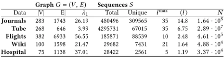
Table 1: Description of empirical data sets, withλ1denoting the largest eigenvalue of the adjacency matrix of graphG,

N =Í

ilibeing the sum of all path lengths,lmaxand⟨l⟩ de-noting maximum and average path length.

GraphG=(V,E) SequencesS Data |V| |E| λ1 Total Unique l

max _{⟨l⟩ N} Journals 283 1743 26.19 480496 309565 35 14.8 1.64·108 Tube 268 646 3.99 4295731 67015 35 6.75 2.89·107 Flights 382 6933 56.55 185871 88539 10 2.48 4.61·105 Wiki 100 1598 21.47 29682 7431 21 1.64 4.88·104 Hospital 75 1138 37.01 28422 2561 5 1.19 3.37·104

We now show that we can use the scores calculated by HYPA to detect paths with anomalous frequencies. We first validate our method in both synthetically generated data with known implanted anomalies and in real data with ground truth path anomaly labels generated by numerical simulation. Then, we apply our method to empirical time series data on transportation, information, and social networks, showing that the under- and over-represented

paths fall into different classes that can be validated using semantic and geographic features.

4.1

Baseline Method

In the below experiments, we compare HYPA to a simple frequency-based anomaly detection (FBAD) of our own design. We note that despite similar problem settings, the methods for hypothesis testing on human trails presented in [8, 44] are not directly comparable with our work because the output is Bayesian evidence for a hy-pothesis on an entire dataset (a single number), whereas we are interested in edge-level analysis. However, in future work we could use HYPA to generate hypotheses to be tested using these meth-ods. Further, we did not compare with a method like [39] because, while based on detecting significant deviations from a Markov chain model, this method assumes that the data is given as one long sequence and detects anomalous subsequences, which does not correspond to any of the datasets we analyze here.

We now briefly describe FBAD and provide more details includ-ing pseudocode in Algorithm 5 of Appendix A.5. FBAD computes the averageµand standard deviationσof path counts and employs a user-defined thresholdαto detect over- and under-represented paths. In particular, a path is labeled as over-represented if its fre-quency exceedsµ+σα, and as under-represented if its frequency is smaller thanµ−σα.

4.2

Synthetic Data

AUC Anomaly length l = 2 l = 3 l = 4 l = 5

Figure 3:HYPA(k)detects injected path anomalies at the cor-rect length with high accuracy. Each curve corresponds to one lengthlof generated anomalous paths, and represents the performance of classifying the anomalous paths using HYPA (left) or the naive FBAD method (right) applied at in-creasing ordersk. HYPA detects the exact generated anom-alies, i.e., performs highly atk=l. FBAD only performs rela-tively well in detecting short sub-paths (e.g.,k=2) of longer anomalies (e.g.,l=5). Averages and standard errors are over 10 independent experiments.

To validate our method, we use a stochastic model generating syn-thetic sets of paths with varying lengths, in which a known set of paths with given lengthlexhibit anomalous frequencies. Adopt-ing the well-known Erdős-Rényi model [21], our model generates paths in a random directed graphGwithnnodes, where pairs of nodes are connected with probabilityp. Following Definition 3.2, the random model generates paths based on an edge-weighted ran-dom walk in ak-th order De Bruijn graph of paths in the random graphG. By selectively changing transition probabilities inTl (cf.

Definition 3.2), we introduce anomalous frequencies for a known set of paths at lengthl. Since all paths longer thanlare generated by a (Markovian) random walk on a De Bruijn graph with orderl, these paths will not exhibit anomalous frequencies beyond those expected from the anomalous frequencies of paths of lengthl. For details of the random path construction, see the pseudocode in Algorithms 3 and 4 in Appendix A.3. In the following we report results for graphsGwithn=50 nodes and an edge probability of p=0.05 (conclusions do not depend on those parameters).

We test whether HYPA detects anomalous path frequencies (i) with high accuracy, and (ii) at the correct lengthlintroduced by our model. To this end, we calculate the performance of HYPA in a binary classification experiment, categorizing path frequencies as anomalous based on variable discrimination thresholdsαfor the HYPA(k)scores at different ordersk. For each thresholdα, we compute the true and false positive rates of detected anomalies w.r.t. the known ground truth and obtain a receiver operating char-acteristic (ROC) curve, for which we can calculate the area under the curve (AUC). For each lengthl∈ [2,5]of generated anomalous paths and each orderk∈ [1,5], we repeat this experiment 10 times. Each curve in Fig. 3 presents the mean and the standard error of theAUCfor anomalies detected at varying ordersk, for a given anomaly lengthl. Fork_,l, we use as ground-truth the paths of lengthkthat either include or are included in an anomalous path of lengthlgenerated by the synthetic model. For eachlwe observe that HYPA with the “correct” orderk=lis able to identify ground truth anomalies with high accuracy (AUC≈0.9, left plot), while the baseline FBAD method is unable to detect path anomalies with high accuracy at any order, regardless of the order used for detection (maxAUC≈0.78, right plot).

4.3

Empirical Data

We now apply our method to five empirical datasets capturing paths in transportation systems, information networks, and dynamic so-cial networks:Tubecomprises sequences of stations traveled in the London Underground [22];Flightscomprise 5% of all travel itineraries of passengers flying in the US in the first quarter of 2018 [48];Journalsrepresent citations between a subset of High-Energy Physics journals [26];Hospitalcontains face-to-face contact sequences of people occupying four roles (patients, nurses, doctors, administrators) in a hospital ward [49]; andWikicontains click-stream data from the “Wikispeedia” game where players had to find a specified target page starting from a given Wikipedia page by following hyperlinks. Basic characteristics of these datasets are presented in Table 1 (see Appendix A.6 for details on filtering and processing of the data).

Detection of ground truth anomalies.As exemplified in Fig. 2(c) and implied by Definition 3.1, path anomalies can, in principle, also be discovered through large-scale numerical simulations. To achieve this for orderkwe can randomize the data by replacing every observed path with a(k−1)-order random walk of the same length starting in the same node. A large number of such simulations generates empirical frequency distributions of all paths with given lengthk. We can then use those distributions to infer which paths in the empirical data are over- or under-represented. A detailed description of this approach can be found in Appendix A.7. While

2 3 4 5 Order 0.0 0.2 0.4 0.6 0.8 1.0 AUC FBAD HYPA

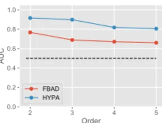
Figure 4: HYPA outperforms FBAD in detecting anomalous paths in the London Tube data. For this data set, ground truth anomalies can be established using computationally expensive numerical simulations. We apply both methods at various orderskand measure their performance in predict-ing the ground truth. At all detection ordersk, HYPA con-siderably outperforms FBAD, illustrating the inadequacy of frequency-based methods for path anomalies.

it is prohibitively expensive for large data sets, it enables us to generate a proxy forground truth path anomaliesin the London Tube data. In this case, each randomized version of the data is generated by performing more than 4.8 million random walks with an average length of 14.8 steps in the (weighted) graph topology. We repeat this multiple times to obtain ground truth labels for over- and under-represented paths (details in Appendix A.7). Repeating the experiment from Section 4.2, these ground truth labels allow us to compare the performance of HYPA against the baseline frequency-based detection (FBAD). We use the London Tube data set for our experiment because its topology is sufficiently small and sparse to allow for this expensive numerical approach. The results in Fig. 4 show that (i) HYPA is able to detect ground truth path anomalies with high accuracy, (ii) our analytical approach outperforms the detection performance of the baseline frequency-based detection (FBAD) at all ordersk, and (iii) we obtain an increase in prediction performance of approximately 30% at orderk=3.

Path motifs.In Fig. 5 we study how anomalous paths detected by HYPA atk=2 are distributed in the three data setsWiki,Journals, andHospital. We focus on five distinct motifs (horizontal axis in plots) where, e.g.ABC# ”represents paths traversing distinct nodes andABA# ”represents paths that start and end in the same node but pass through another node. While Fig. 5 highlights the absence of a universal pattern of motif anomalies across systems, some of the observed differences can be intuitively attributed to system-specific mechanisms. For instance, paths of the typeABA# ”are among the most over-represented paths inWiki, which is likely a result of users using the ‘back’ button of their browser while playing the game. InJournals, citation paths of the typeABC# ”through three distinct journals are both most over-represented and least under-represented. This indicates (i) a hierarchy in journals in terms of knowledge flows through citations (papers inAimplicitly rely on papers inC) and (ii) that knowledge flow is preferentially routed through certain sets of (probably multi-disciplinary) journalsB.

Tube Geographic Hypothesis.We next use HYPA to test a hy-pothesis about the geographic embedding and over- and under-represented paths inTube. Intuitively, we expect people to use

Under Expected Over Hospital Journals Wiki

AAA ABA AAB ABB ABC AAA ABA AAB ABB ABC

0.00 0.25 0.50 0.75 1.00 Fraction

AAA ABA AAB ABB ABC

0.00 0.25 0.50 0.75 1.00 Motifs_AAA ABA AAB ABB ABC

Figure 5: The distribution of over and under represented paths (k =2) across motifs, i.e., recurrenttypesof paths, is system dependent. For instance, in click stream data the mo-tifABAis over-represented much more than the others due to the user hitting the’back’button in the browser. The dis-crimination threshold used for detection wasα=0.01.

public transportation like the London Underground preferentially for longer distance trips, such as commutes to and from work, while avoiding trips with very short, walk-able distances. This leads to the hypothesis that over-represented itineraries span larger geographic distances compared to those that are under-represented.

We use HYPA to test this hypothesis. We first compute HYPA(k) scores for valuesk = 1, . . . ,6. We then detect over- and under-represented paths based on discrimination thresholdα=0.001. We can use the detected anomalies to generate a decomposition of a k-th order De Bruijn graph model of paths based on under- and over-represented edge weights. The resulting decomposition fork=2 are shown in Fig. 6 (left column), where the nodes are placed according to geographic positions of London Tube stations. The network of under-represented paths (top) exhibits high clustering and an absence of long chains, highlighting that it is predominantly paths spanning short geographic distances that are under-represented. In contrast, the network of over-represented paths (bottom) shows long chains, which supports the hypothesis that paths spanning longer distances are occurring more often than expected at random. To substantiate this intuition, in Fig. 6 we show how geographic distances between start and end stations in over- and under-represen-ted itineraries atk=2 are distributed. The distance distribution of under-represented itineraries is shifted towards smaller distances, while the over-represented distribution is shifted towards larger distances, which supports our hypothesis. We find that the shift in distance distribution at order two is significant, witnessed by a p-value≈0 of a Mann-Whitney U-test (Table 2). Because the null model allows for paths starting and ending at the same node, there is a peak in the distribution of under-represented paths (see Fig. 6) at distance zero. This is due to such paths being absent in the data. Atk >2 paths starting and ending at the same node are not present, hence repeating the test provides a better support for the geographic hypothesis. As shown in Table 2, indeed the over-represented trips are longer on average.

Efficiency and Balance in Flight Itineraries.We now show how HYPA can be used to test hypotheses about specific types of paths. We demonstrate this in a large data set containing flight itineraries of airline passengers in the United States. Our first hypothesis is that return flights (ABA) are significantly over-represented, since

Table 2: The median distance in kilometers between origins and destinations is significantly larger for over-represented paths of lengthkcompared to under-represented paths in the London Tube, as shown by thep-value one-sided Mann-Whitney U-test. The discrimination threshold on HYPA (2) scores wasα=0.001. HYPA(k) k=2 k=3 k=4 k=5 k=6 Under [km] 0.00 2.38 3.29 4.60 5.43 Over [km] 2.20 2.93 3.79 5.21 5.63 p-value <10−170 <10−7 <10−4 0.006 0.08 Density

Figure 6: For any orderkand discrimination thresholdα, HYPA acts as a filter on thekth order De Bruijn graph, sep-arating over-represented (blue) and under-represented (red) paths of lengthk. In the Tube data, Under-represented paths detected by HYPA are tightly clustered, corresponding to avoidance of geographically short trips. Over-represented paths are arranged in chains, corresponding to longer dis-tance trips (as in daily suburban commutes). On the right, we show a histogram of geographic distances, to illustrate that both over- and under-represented paths detected by HYPA correlate with the geography of the system.

passengers often leave from and return to the same airport. We first compute HYPA scores fork=2. We then separate return from non-return flights and compute the fraction of over-represented paths in each for varying discrimination thresholdsα. The results in Table 3 support the hypothesis that return flights are strongly over-represented with respect to the random baseline.

Table 3: Fractions of over-represented paths (k = 2) be-tween airports for return flights (5840 unique paths) and non-return flights (409254 unique paths) at different dis-crimination thresholdsα.

α 0.05 0.01 0.001 0.0001 0.00001 Return 0.915 0.851 0.760 0.688 0.628 Non-return 0.340 0.130 0.023 0.004 0.001 However, we still observe a number of over-represented non-return flight paths. We hypothesize that many over-represented paths connect small airports to large airports via regional hubs. This means that a relatively short distance trip (e.g. from ORL to ATL) is

required before a flight from the regional hub to a relatively distant destination (e.g. ATL to LAX). Rather than classifying airports by their size and role in the network, we test this hypothesis by defin-ingdistance balance, a measure that captures to what extent one leg of a trip dominates the total trip distance. In a perfectly balanced trip

(ABC), the distance of the two legs is equal, e.g.d(A,B)=d(B,C). The most common example of a perfectly balanced trip is the return trip, whereA=C. In an imbalanced trip, one of the legs of the trip is much larger. We define balance by the ratiod(A,B)−d(B,C)

d(A,B)+d(B,C). It approaches -1 or 1 when the distance of one leg of the trip is much greater than on the other. We expect flights with extreme values to be over-represented as they represent long distance flights that start from small, local airports, fly a short distance to a regional hub, then on to a much further off destination (as well as the reverse). The distribution of balance for over- and under-represented paths of length two (α=0.05) is shown in Fig. 7 (top right). We find very few under-represented flights near extreme values of balance, while a larger fraction of over-represented paths are found near -1 and 1. This supports our hypothesis that unbalanced flights tend to be more over-represented than balanced flights.

We conclude this analysis by formulating hypotheses based on a notion ofefficiencyfor airline trips. We measure efficiency as the ratio of the distance between source and destination,d(A,C), with the actual flight distance,d(A,B)+d(B,C). Using this measure, a straight line between airports A, B and C would have a maxi-mum efficiency of 1, while a low efficiency trip implies that the actual flight distance is much larger than the straight line distance between the origin and destination. We hypothesize that highly efficient paths are over-represented, while inefficient paths are under-represented in the data. The bottom left plot of Fig. 7 shows a large peak in the fraction of under-represented paths at very low efficiency, then a steady decrease in under-represented paths as efficiency increases. In the bottom right figure we see that after return flights are accounted for (peak at efficiency 0), the fraction of over-represented paths increases monotonically with efficiency. These results indicate that more efficient paths are indeed more likely to be over-represented, and that the more efficient a path is, the less likely it is to be under-represented.

4.4

Scalability

We finally validate the theoretical analysis of computational com-plexity in section 4.4 through an experimental evaluation of scal-ability in empirical data. We measure the time needed to detect path anomalies for (i) varying orderskin a data set of fixed sizeN and (ii) a fixed orderkand data with varying sizeN. Fig. 8 reports the time needed to run HYPA on a single core of an Intel i7-7600U CP U. All values are averages of ten measurements. The left panel in Fig. 8 confirms that the runtime of our algorithm scales as an exponent ofk, where the basis of the exponent depends on the algebraic connectivity of the graph. We note however that, even for a data set with more than four million paths the detection of anomalies up to length eight takes less than two minutes. The right panel in Fig. 8 confirms that our analytical approach is suitable for large data sets. In particular, the experimental results are aligned with our theoretical analysis of computational complexity in Sec-tion 3.2, which predicts that below a critical sum of path lengths

A

B

C

1.0 0.5 0.0 0.5 1.0 Distance balance, d(A, B) d(B, C)

d(A, B) + d(B, C) 0.00 0.25 0.50 0.75 1.00 1.25

Density of HYPA(2) scores

Under Over

0.00 0.25 0.50 0.75 1.00 Distance efficiency, d(A, C)

d(A, B) + d(B, C) 0.00 0.01 0.02 0.03 Fraction under-represented 0.0 0.2 0.4 0.6 0.8 1.0 Distance efficiency, _{d(A, B) + d(B, C)}d(A, C) 0.2

0.4 0.6 0.8

Fraction over-represented

Figure 7: Top-right: extreme values ofbalancecorrespond to over-represented paths, confirming that short flights fol-lowed by long flights are typical (e.g. flights to a regional hub, then a national hub). Bottom-left: The fraction of over-and under-represented paths in data on flight itineraries varies with the efficiency of the itinerary, which we define as the ratio of the straight line distanced(A,C)between the ori-gin and the destination and the total flight distanced(A,B)+ d(B,C). After return flights are accounted for, the fraction of under-represented paths decreases with efficiency, and vice versa for over-represented paths.

N, the runtime of HYPA is dominated by the number of paths of lengthk. This explains why for small values ofNwe observe an exponential increase of runtime as the size of thek-dimensional De Bruijn graph model approaches the theoretical upper limit of

|V|2λk

1. For large values ofN, the runtime of HYPA is dominated by a linear term that is due to the single pass through the data, while the calculation of HYPA scores is independent of the size of the data. This confirms that the analytical approach underlying our algorithm makes it suitable to analyse big time series data on networks. 2 4 6 8 HYPA order 100 101 102 Runtime [sec] 0 200000 400000

N

Figure 8: Empirical scalability of HYPA. Left: Required time to detect path anomalies of lengthkfor the Tube data. Right: Runtime in Flights data for detection orderk =1and vary-ing data sizeN randomly sampled from the data. All data points correspond to the mean of ten repeated measure-ments, with the standard deviations shown as bars.

5

CONCLUSION

We have presented a novel approach for the unsupervised detection of path anomalies in time series data on networks. Providing a new theoretical basis for anomaly detection in graphs, our work ad-vances the state-of-the-art in multiple directions. We first introduce the problem of path anomaly detection and show that it cannot be addressed by existing frequency-based anomaly detection tech-niques. Projecting paths in a (first-order) graph onto higher-order De Bruijn graphs, we show that path anomaly detection can be reduced to the detection of anomalous edge weights in a higher-order graph space. Building on an analytically tractable null model of higher-order De Bruijn graphs, we obtain a parameter-free and scalable method that allows us to assess statistical deviations in the frequencies of paths traversing the nodes of a graph.

Compared to works focused on finding optimal higher-order models of time series data, our approach allows to detect which individual paths exhibit significant deviations from a random base-line. Our method opens new perspectives for model order reduction in higher-order network models, which can help to alleviate some of the scalability issues. To facilitate the reproducibility of our find-ings and applications of our method in real scenarios, a_python implementation of our framework will be made available online [7].

ACKNOWLEDGEMENTS

Ingo Scholtes acknowledges support by the Swiss National Science Foundation, grant 176938. LaRock and Eliassi-Rad were supported in part by NSF IIS-1741197, the Army Research Laboratory Cooper-ative Agreement W911NF-13-2-0045, and the Under Secretary of Defense for Research and Engineering under Air Force Contract No. FA8702-15-D-0001. Any views, opinions, findings, conclusions or recommendations expressed in this material are solely those of the authors.

REFERENCES

[1] R. Agrawal and R. Srikant.Mining sequential patterns. InICDE, pages 3–14, 1995.

[2] L. Akoglu and C. Faloutsos. Event detection in time series of mobile communica-tion graphs. In_{Army Science Conference}, pages 77–79, 2010.

[3] L. Akoglu, H. Tong, and D. Koutra. Graph based anomaly detection and descrip-tion: a survey. volume 29, pages 626–688, 2015.

[4] M. Atzmueller. Detecting community patterns capturing exceptional link trails. In_ASONAM, pages 757–764, 2016.

[5] M. Atzmueller, A. Schmidt, and D. Arnu.Sequential modeling and structural anomaly analytics in industrial production environments. In_LWDA, pages 283–290, 2016.

[6] M. Atzmueller, A. Schmidt, and M. Kibanov. Dashtrails: an approach for modeling and analysis of distribution-adapted sequential hypotheses and trails. In_WWW, pages 553–558, 2016.

[7] B. authors. hypa software package. to be published at gitHub.com, 2019. [8] M. Becker, F. Lemmerich, P. Singer, M. Strohmaier, and A. Hotho. Mixedtrails:

Bayesian hypothesis comparison on heterogeneous sequential data.Data Mining

and Knowledge Discovery, 31(5):1359–1390, 2017.

[9] R. Bertens, J. Vreeken, and A. Siebes. Keeping it short and simple: Summarising complex event sequences with multivariate patterns. InKDD, 2016.

[10] C. C. Bilgin and B. Yener. Dynamic network evolution: Models, clustering, anomaly detection.IEEE Networks, 2006.

[11] B. Boden, S. Günnemann, and T. Seidl. Tracing clusters in evolving graphs with node attributes. InCIKM, pages 2331–2334, 2012.

[12] I. Cadez, D. Heckerman, C. Meek, P. Smyth, and S. White. Visualization of navigation patterns on a web site using model-based clustering. In_KDD, pages 280–284, 2000.

[13] G. Casiraghi and V. Nanumyan. Generalised hypergeometric ensembles of ran-dom graphs: The configuration model as an urn problem. _{arXiv:1810.06495}

[physics], 2018.

[14] G. Casiraghi, V. Nanumyan, I. Scholtes, and F. Schweitzer. From relational data to graphs: Inferring significant links using generalized hypergeometric ensembles. InSocial Informatics, pages 111–120, 2017.

[15] S. Chakrabarti, S. Sarawagi, and B. Dom. Mining surprising patterns using temporal description length. InVLDB, volume 98, pages 606–617, 1998. [16] V. Chandola, A. Banerjee, and V. Kumar. Anomaly detection: A survey._ACM

computing surveys, 41(3):15, 2009.

[17] V. Chandola, A. Banerjee, and V. Kumar. Anomaly detection for discrete se-quences: A survey._{IEEE TKDE}, 24(5):823–839, 2012.

[18] V. Chandola, V. Mithal, and V. Kumar. Comparative evaluation of anomaly detection techniques for sequence data. In_ICDM, pages 743–748, 2008. [19] N. G. de Bruijn. A combinatorial problem._{Koninklijke Nederlandse Akademie v.}

Wetenschappen, 49:758–764, 1946.

[20] M. El-Sayed, C. Ruiz, and E. A. Rundensteiner. Fs-miner: efficient and incremental mining of frequent sequence patterns in web logs. In_WIDM, 2004.

[21] P. Erdos and A. Rényi. On the evolution of random graphs. _{Publ. Math. Inst.}

Hung. Acad. Sci, 5(1):17–60, 1960.

[22] T. for London. Rolling origin and destination survey (rods)database. http://www. tfl.gov.uk/info- for/open- data- users/our- feeds, 2014.

[23] E. N. Gilbert. Random graphs.The Annals of Mathematical Statistics, 30(4):1141– 1144, 1959.

[24] M. Gupta, J. Gao, C. C. Aggarwal, and J. Han. Outlier detection for temporal data: A survey.IEEE TKDE, 26(9):2250–2267, 2014.

[25] R. Gwadera, M. Atallah, and W. Szpankowski. Markov models for identification of significant episodes. InSDM, pages 404–414, 2005.

[26] INSPIRE. Inspire hep. http://inspirehep.net/info/hep/api, 2018.

[27] E. Keogh, S. Lonardi, C. A. Ratanamahatana, L. Wei, S.-H. Lee, and J. Handley. Compression-based data mining of sequential data.Data Mining and Knowledge

Discovery, 14(1):99–129, 2007.

[28] R. Lambiotte, M. Rosvall, and I. Scholtes. From networks to optimal higher-order models of complex systems._{Nature Physics}, 15:313–320, April 2019. [29] T. Lane and C. E. Brodley. An empirical study of two approaches to sequence

learning for anomaly detection._MLJ, 51(1):73–107, 2003.

[30] R. Laxhammar and G. Falkman. Online learning and sequential anomaly detection in trajectories._TPAMI, 36(6):1158–1173, 2014.

[31] F. Lemmerich, M. Becker, P. Singer, D. Helic, A. Hotho, and M. Strohmaier. Mining subgroups with exceptional transition behavior. In_KDD, pages 965–974, 2016. [32] I. Melnyk, B. Matthews, H. Valizadegan, A. Banerjee, and N. Oza. Vector

autore-gressive model-based anomaly detection in aviation systems. J. of Aerospace

Information Systems, pages 161–173, 2016.

[33] J. K. Merikoski. On the trace and the sum of elements of a matrix.Linear Algebra

and its Applications, 60:177 – 185, 1984.

[34] M. Molloy and B. Reed. A critical point for random graphs with a given degree sequence.Random Structures & Algorithms, 6(2-3):161–180, 1995.

[35] C. C. Noble and D. J. Cook. Graph-based anomaly detection. InKDD ’03, 2003. [36] G. Palla, N. Páll, A. Horváth, K. Molnár, B. Tóth, T. Kováts, G. Surján, T. Vicsek,

and P. Pollner. Complex clinical pathways of an autoimmune disease. J. of

Complex Networks, 6(2):206–214, 2017.

[37] T. P. Peixoto and M. Rosvall. Modelling sequences and temporal networks with dynamic community structures.Nature communications, 8(1):582, 2017. [38] M. Rosvall, A. V. Esquivel, A. Lancichinetti, J. D. West, and R. Lambiotte. Memory

in network flows and its effects on spreading dynamics and community detection.

Nature communications, 5, 2014.

[39] R. Sadoddin, J. Sander, and D. Rafiei. Finding Surprisingly Frequent Patterns of Variable Lengths in Sequence Data. In_{Proceedings of the 2016 SIAM International}

Conference on Data Mining, pages 27–35. Society for Industrial and Applied Mathematics, June 2016.

[40] V. Salnikov, M. T. Schaub, and R. Lambiotte. Using higher-order Markov models to reveal flow-based communities in networks._{Sci. Rep.}, 6:23194, 2016. [41] I. Scholtes. When is a network a network?: Multi-order graphical model selection

in pathways and temporal networks. In_KDD, pages 1037–1046, 2017. [42] I. Scholtes, N. Wider, R. Pfitzner, A. Garas, C. J. Tessone, and F. Schweitzer.

Causality-driven slow-down and speed-up of diffusion in non-markovian tempo-ral networks.Nature Communications, 5:5024, 2014.

[43] S. Servan-Schreiber, M. Riondato, and E. Zgraggen.Prosecco: Progressive se-quence mining with convergence guarantees. InICDM, pages 417–426, 2018. [44] P. Singer, D. Helic, A. Hotho, and M. Strohmaier. Hyptrails: A bayesian approach

for comparing hypotheses about human trails on the web. InWWW, pages 1003–1013, 2015.

[45] P. Smyth.Clustering sequences with hidden markov models. InNIPS, pages 648–654, 1997.

[46] A. Tajer, V. V. Veeravalli, and H. V. Poor. Outlying sequence detection in large data sets: A data-driven approach._{IEEE Signal Processing Magazine}, 31(5):44–56, 2014.

[47] E. Tonnelier, N. Baskiotis, V. Guigue, and P. Gallinari. Anomaly detection in smart card logs and distant evaluation with twitter: a robust framework.

Neuro-computing, 298:109–121, 2018.

[48] R. TransStat. Origin and destination survey database. http://www.transtats.bts. gov/Tables.asp?DB_ID=125, 2018.

[49] P. Vanhems, A. Barrat, C. Cattuto, J. Pinton, and N. Khanafer. Estimating potential infection transmission routes in hospital wards using wearable proximity sensors.

PLoS ONE, 8(9):e73970, 09 2013.

[50] S. Walk, P. Singer, and M. Strohmaier. Sequential action patterns in collaborative ontology-engineering projects: A case-study in the biomedical domain. In_CIKM, pages 1349–1358, 2014.

[51] R. West and J. Leskovec. Human wayfinding in information networks. In_WWW, pages 619–628, 2012.

[52] J. Xu, T. L. Wickramarathne, and N. V. Chawla. Representing higher-order dependencies in networks._{Science Advances}, 2(5), 2016.

[53] D. Zhou, J. He, Y. Cao, and J.-s. Seo. Bi-level rare temporal pattern detection. In

ICDM, pages 719–728, 2016.

A

SUPPLEMENTARY MATERIAL

To facilitate reproducibility, we use this supplement for the fol-lowing: (i) describe in detail the algorithm we use to redistribute values in theΞmatrix (Section 3); (ii) provide a proof for Lemma 1, which was omitted from the main text due to space constraints; (iii) provide details and pseudocode for the synthetic model used for the experiment in Fig. 3; (iv) explain in detail how the results in Fig. 3 were generated; (v) provide pseudocode for the naive base-line method FBAD; (vi) provide details of the construction and preprocessing of the real world datasets (Section 4); and finally (vii) describe in more detail the procedure we used to generate ground truth path anomalies.

A.1

Ξ

Redistribution

In Section 3.2 we briefly describe a simple algorithm to redistribute the values in the matrixΞsuch that it respects the constraints imposed by thek-order De Bruijn graph while also preserving the weighted in- and out-frequencies of thek-order nodes when used for sampling. Algorithm 2 shows the exact procedure we employ.

Algorithm 2fitXi(Gk, tolerance):Adjust entries ofΞto match ex-pected frequencies (based onΞ) to observed frequencies (based on W)within “tolerance” error.

Input: Gk(k-order De Bruijn graph), tolerance Output:Ξ

1: f_vout←Í_xf(v,x) # weighted out-degrees 2: f_vin←Í_xf(x,v) # weighted in-degrees 3: m←Í_vf_vout # sum of all weights

4: Ξvw←f_vout·f_win # initialize matrix for allv,w∈Gk 5: M←Í_vwΞvw

6: ifedge(v,w)not possible inGkthen

7: Ξvw←0 # ensure edge(v,w)cannot be sampled 8: repeat 9: bf in v← Í xΞxv m Í M

vwΞvw # Expectation for in-degrees

10: Ξvw←Ξvw·f in w b fin w

# Correction for in-degrees

11: bf_vout← Í

xΞv x

m Í M

vwΞvw # Expectation for out-degrees

12: Ξvw←Ξvw·f out v b fout v

# Correction for out-degrees

13: untilRMSE(fout,fb

out

)+RMSE(fin,fb

in

) ≤tolerance 14: return Ξ

A.2

Proof of Computational Complexity

1, whereλ1is the leading eigenvalue of the binary adjacency matrix ofG.

Proof. We first note that for a fully connected graphGwith|V| nodes andE=V2we trivially have∆k(G)=|V|k+1. This follows from the fact that every possible sequence ofk+1 nodes is a path of lengthkin a full graph, i.e. ak-th order De Bruijn graph model has|V|k+1edges.

Let us now consider a graphGwith arbitrary topology and letA be the binary adjacency matrix ofG, where one-elements indicate

the presence and zero-elements indicate the absence of an edge. We can compute the number of distinct paths of lengthkinGas Í

iÍj(Ak)ij, whereAkis thek-th power of adjacency matrixA. This directly follows from the definition of matrix multiplication, leading to the fact that each element(Ak)ijin thek-th power ofA counts distinct paths of lengthkbetween nodesiandj.

To prove the lemma, we use the following two facts. First, the sum of all elements in any matrixBis equal to tr(JB), i.e., the sum ofdiagonal elements in the matrix productJB, whereJis the|V| × |V|all-ones matrix. Second, ifB,Care positive semi-definite matrices, from the Cauchy-Schwartz inequality follows tr(CB) ≤tr(C)tr(B)[33]. We can thus write:

∆k(G)= |V| Õ i=1 |V| Õ j=1 (Ak)ij=tr(JAk) ≤tr(J) ·tr(Ak)

We now recall (i) that the trace of any square matrix is equal to the sum of its eigenvalues, (ii) that the eigenvalue sequence of an|V| × |V|all-one matrixJis|V|,0, . . . ,0, and (iii) that the eigenvalues of thek-th powerAkof a matrix are thek-th powers of eigenvalues ofA. We can thus write:

∆k(G) ≤tr(J) ·tr(Ak)=|V| · |V| Õ

i=1 λk_i

whereλ_i are the (not necessarily unique) eigenvalues of A. Without loss of generality, we assume that the eigenvalues are given in descending order, i.e.λ1 ≥ . . . ≥ λ|V|. Hence, an up-per bound∆k(G) ≤ |V|2λk

1 can be derived based on the largest eigenvalueλ1of the adjacency matrix ofG. We note that for the special case of a fully connected graph, whereA = J, we have

∆k(G)=tr(JAk)=tr(Jk+1)=λk+1

1 =|V| k+1

and we thus recover

the trivial case from above. □

A.3

Synthetic data

In Section 4, we briefly described a model that generates pathways with injected correlation patterns, but could not include the pseu-docode due to space constraints. Algorithm 3 presents pseupseu-docode for constructing the graph topology, and Algorithm 4 shows how we generate a walk on this topology.

Algorithm 3SyntheticModel(N,p,f,k):Generates a directedG_N,p graph and marks fractionf of lengthkpathways throughG anoma-lous.

Input: N (number of nodes),p(connection probability),f (fraction of anomalous pathways),k(anomaly order)

Output:G(weighted topology), paths (paths marked anomalous) 1: G←directedER(N, p)

2: for(i,j) ∈Gdo

3: Gi,j←unif(1, 20) # Assign edge weight 4: Gk←DeBruijnGraph(G,k)

5: anom-paths =∅ 6: forpath∈Gkdo 7: ifr andom()<f then

8: anom-paths←path # mark path anomalous 9: return G, anom-paths

Algorithm 4SyntheticWalk(G,paths,l):Given a weighted first-order topologyGand list of anomalous paths, generate a (potentially anomalous) random walk of lengthl.

Input: G(weighted network topology), paths (paths throughGmarked anomalous), l (length of walk)

Output:path

1: u←uniform random node 2: path =[u]

3: whilej<ldo

4: ifuis on an anomalous paththen

5: whilej<land nodes remain on anomalous pathdo 6: v←next node on anomalous path

7: Appendvto path

8: j←j+1 9: else

10: v←v∈Nu # Pr(u,v) ∝edge weightG_u,v 11: Appendvto path

12: j←j+1 13: u=v 14: return path

A.4

ROC Curves used to compute AUC

In Fig. 3, we presented area under the curve results for a binary classification experiment where we used HYPA to predict ground truth over- and under-represented paths. In this section, we clarify the procedure for generating these results.

First, we use Algorithms 3 and 4 to generate a dataset with injected anomalies at orderl. Then, for each value ofk, we compute HYPA(k)scores, and for increasingαfrom 0 (nothing detected) to 1 (everything predicted as significant), we threshold the HYPA(k) scores to classify the ground truth over- and under-represented paths. We compute the true and false positive rates for eachα, which results in a single ROC, where each point is a combination ofkandα. We get an ROC for every combination of HYPA order (k) and anomaly order (l). Finally, we compute the area under these curves and report averages and standard deviations over many randomly generated datasets, which is what is reported in Fig. 3.

A.5

Naive Baseline Method

Here we provide pseudocode for the Frequency Based Anomaly Detection (FBAD) method.

Algorithm 5FBAD(S,k,α):Given path dataS, orderk, and scaling factorα∈_R, compute anomalies based on the distribution of order-k edgeweights.

Input: S(input path data),k(desired anomaly order),α(scaling factor) Output:G(k-th order network with anomaly-labeled transitions)

1: G←DeBruijnGraph(S,k) 2: µ←average of edge weights inG

3: σ←standard deviation of edge weights inG 4: foredgeeinGdo

5: iffrequency(e)>µ+σ αthen 6: Labeleover-represented 7: else iffrequency(e)<µ−σ αthen 8: Labeleunder-represented 9: return Labeled graphG

A.6

Data

In Table 1 we presented some statistics of our datasets. Below we provide more detail about the specifics of how each dataset was constructed and processed before our analysis.

Tube.The Tube data is given in the form of origin-destination statistics between stations [22]. We then use these statistics in conjunction with the first-order topology of the Tube network to construct pathways by computing the shortest path between each origin and destination, then assuming riders take this path. If there are multiple shortest paths between an origin and a destination, the observed paths are distributed across them.

Journal Citations.The journal citation data begins with a cita-tion graph [26], where a directed link is drawn from paperito paperjificitesj. We then enforce that this graph is directed and acyclic by removing “backlinks”, meaning links from nodeitoj such thatjwas published afteri. Pathways of citations are then constructed by walking from a “source” paper (a paper which was never cited in the dataset) to a “sink” paper (a paper that didn’t cite any other papers in the dataset). Reversing the order of this pathway results in a chronological “citation flow” from the sink (the oldest paper) to the source (the newest paper). These sequences of papers are then projected using a mapping from individual paper to publication venue, giving us sequences of journals that cited one another through time. Our analysis is of this projected data.

Flights. The flights dataset is given in the form of “itineraries”, which correspond to tickets purchased together by a particular cus-tomer [48]. Each pathway is a sequence of airports corresponding to source, layovers, and destination. Our dataset is constructed by taking a uniform 5% sample of these pathways from the first quarter of 2018.

Hospital.The Sociopatterns data is a sequence of time stamped edges representing interactions between nurses, doctors, adminis-trative staff and patients in a hospital [49]. We define a pathway by a 20-second inter-event time, meaning that if 2 interactions in-cluding a common person happened within 20 seconds, they are combined into a path. A path ends when 20 seconds passes without the last person to interact having a subsequent interaction.

Wikispeedia.We focus our analysis of the Wikispeedia data [51] on the pathways which represent finished games. In the full dataset, the number of observed pathways is too small relative to the size and density of the underlying article graph to compute meaningful statistics across the entire network. Due to this, we only analyze games which traverse the