Javed, Abbas; Larijani, Hadi; Ahmadinia, Ali; Emmanuel, Rohinton
Published in:
Probability in the Engineering and Informational Sciences DOI:
10.1017/S0269964817000201
Publication date: 2017
Document Version Peer reviewed version
Link to publication in ResearchOnline
Citation for published version (Harvard):
Javed, A, Larijani, H, Ahmadinia, A & Emmanuel, R 2017, 'Random neural network learning heuristics', Probability in the Engineering and Informational Sciences, vol. 31, no. 4, pp. 436-456.
https://doi.org/10.1017/S0269964817000201
General rights
Copyright and moral rights for the publications made accessible in the public portal are retained by the authors and/or other copyright owners and it is a condition of accessing publications that users recognise and abide by the legal requirements associated with these rights.
Take down policy
If you believe that this document breaches copyright please view our takedown policy at https://edshare.gcu.ac.uk/id/eprint/5179 for details of how to contact us.
F
Abstract
The Random Neural Network is a probabilitsic queueing theory based model for artificial neural networks, and it requires the use of optimisation algorithms for training. Commonly used gradient descent learning algorithms may reside in local minima, evolutionary algorithms can be also used to avoid local minima. Other techniques such as artificial bee colony, particle swarm optimisation, and differential evolution algorithms also perform well in finding the global minimum but they converge slowly. The sequential quadratic programming optimisation algorithm can find the optimum neural network weights, but can also get stuck in local minima. We propose to overcome the shortcomings of these various approaches by using hybridised artificial bee colony/particle swarm optimisation and sequential quadratic programming. The resulting algorithm is shown to compare favorably with other known techniques for training the Random Neural Network. The results show that hybrid artificial bee colony learning with sequential quadratic programming outperforms other training algorithms in terms of mean squared error and normalised root mean squared error.
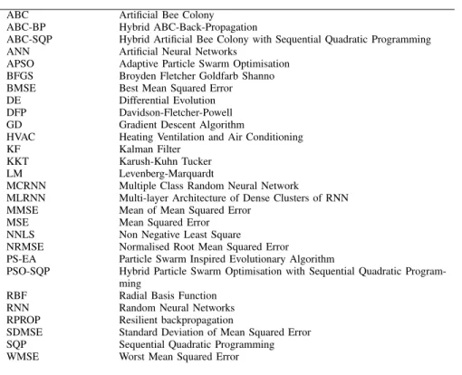
TABLE 1. List of Acronyms and Abbreviations
ABC Artificial Bee Colony
ABC-BP Hybrid ABC-Back-Propagation
ABC-SQP Hybrid Artificial Bee Colony with Sequential Quadratic Programming
ANN Artificial Neural Networks
APSO Adaptive Particle Swarm Optimisation
BFGS Broyden Fletcher Goldfarb Shanno
BMSE Best Mean Squared Error
DE Differential Evolution
DFP Davidson-Fletcher-Powell
GD Gradient Descent Algorithm
HVAC Heating Ventilation and Air Conditioning
KF Kalman Filter
KKT Karush-Kuhn Tucker
LM Levenberg-Marquardt
MCRNN Multiple Class Random Neural Network
MLRNN Multi-layer Architecture of Dense Clusters of RNN
MMSE Mean of Mean Squared Error
MSE Mean Squared Error
NNLS Non Negative Least Square
NRMSE Normalised Root Mean Squared Error
PS-EA Particle Swarm Inspired Evolutionary Algorithm
PSO-SQP Hybrid Particle Swarm Optimisation with Sequential Quadratic Program-ming
RBF Radial Basis Function
RNN Random Neural Networks
RPROP Resilient backpropagation
SDMSE Standard Deviation of Mean Squared Error
SQP Sequential Quadratic Programming
WMSE Worst Mean Squared Error
1 INTRODUCTION
Erol Gelenbe Gelenbe [26, 27] proposed a new class of artificial neural networks (ANN) called Random Neural Networks (RNN) in which signals are either positive or negative spikes or “customers”. The RNN is based on probability theory and belongs to the family of Markovian queuing networks. It is a special case of G-networks
Gelenbe [28, 29, 32], Henderson [54] in queueing theory. In Gelenbe [29] it was shown how “signals” can trigger the movement of customers in a queue and in Gelenbe and Fourneau [40] resets were introduced, and in Fourneau et al. [22] G-networks were extended to multiple classes of positive and negative customers, and generalised in Gelenbe and Labed [44] to include multiple classes. Stability conditions for the G-network was developed in Gelenbe and Schassberger [46].
RNNs are easy to implement in hardware as its neurons can be represented by simple counters Cerkez et al. [18], Abdelbaki et al. [2], and in Abdelbaki [1] the performance of the RNN was compared with conventional with ANNs for unseen patterns not covered in the training data, and found that the RNN accurately measured the output while the ANN failed to predict it accurately. Similarly in Mohamed and Rubino [69], the authors compared RNNs with ANNs and showed that training time for RNNs is greater than ANNs but the RNN outperformed the ANN during run-time. The authors further showed that the RNN had a strong generalisation capability for the patterns not covered in the training phase. ANNs are sensitive to the number of hidden neurons and over-training allows ANNs to memorise the patterns but yiels very poor generalisation for new inputs.
Much recent work has linked the RNN and G-Networks to modeling and simulation in various areas. In Gelenbe and Marin [45], Gelenbe [35] similar models derived from energy or G-Networks are used to represent energy consumption in sensor networks, while Gelenbe and Ceran [37] consider energy distribution and its optimisation. Other work has modelled multiple users of energy using G-Networks to determine the optimum flow of different sources of energy to distinct consumers Gelenbe and Ceran [38] and has derived fast and efficient computational algorithms for this purpose Ceran and Gelenbe [17]. In Gelenbe [33, 34, 36] similar point process models are used for communications with spintronics, while Wang and Gelenbe [81] uses the RNN for smart routing in networks, as well as for building Software Defined Networks Francois and Gelenbe [23] that optimise quality of service (QoS). In Bi and Gelenbe [14], Akinwande et al. [6], Bi et al. [13] the RNN isused for smart routing of evacuees in emergencies, while Abdelrahman and Gelenbe [4] studies the movement of individuals or animals in a random environment.
Many applications of the RNN have been reported in Gelenbe [29, 31], including for optimisation Cancela et al. [16], Zhong et al. [86], pattern recognition Abdelbaki et al. [3], Gelenbe et al. [41], image processing Gelenbe et al.
[39], Lu and Shen [68], Bakirciouglu et al. [9], communication systems Mohamed and Rubino [69], ¨Oke and Loukas
[70], multimedia server modelling Gelenbe and Shachnai [47], video compression Cramer et al. [20], routing for packet networks in Gelenbe and Kazhmaganbetova [43], Wang and Gelenbe [83] and emergency management in Gelenbe and Wu [50]. Recently in Wang and Gelenbe [80, 82], Gelenbe and Wang [49], Wang et al. [79], Brun et al. [15] the authors used RNNs with reinforcement learning for dynamic task allocation in Cloud servers and routing in multi-hop overlay networks. An intelligent internet search assistant based on the RNN was presented in Serrano and Gelenbe [74]. Multi-layer classifiers and auto-encoders based on the RNN were developed in Gelenbe and Yin [51]. Many researchers have used the Gradient Descent (GD) algorithm Gelenbe [30] for learning the weights of RNN models. The GD algorithm is easier to implement but zigzag behaviour may occur near the local minimum and in case of multiple local minima shown in Figure 1, the GD algorithm may learn suboptimal weights. In our previous work Javed et al. [61, 63, 62], we proposed the application of the hybrid particle swarm optimisation with sequential quadratic programming (PSO-SQP) algorithm for training a smart controller for the estimation of occupancy, thermal comfort based thermostat and heating ventilation and air conditioning (HVAC) controller. Results showed that the GD algorithm was unable to train the RNN model, while the PSO-SQP training algorithm gave satisfactory results. In this work, we propose a novel application of the artificial bee colony (ABC) and hybrid artificial bee colony with sequential quadratic programming (ABC-SQP) algorithm for training the RNN. ABC algorithm is simple and robust and it has good exploration and exploitation capabilities in searching global optima. Sequential quadratic programming (SQP) optimisation algorithm can find the optimum weights but in presence of global minima it can get stuck in local minima. The problem of slow convergence of ABC and local minima problem of SQP optimisation can be overcame by hybridisation of ABC and SQP optimisation algorithms. Initially, the RNN is trained with ABC algorithm and then weights learned from the ABC algorithm are used as initial start points for the SQP optimisation algorithm in order to find the optimal weights. The performance of ABC, PSO, differential evolution (DE), GD, ABC-SQP, PSO-SQP for seven different problem sets on the basis of mean squared error (MSE), normalised root mean squared error (NRMSE), number of iterations, and time required by each algorithm is analysed.
The main contributions of this paper are:
• A novel approach of using the ABC algorithm for training a RNN model is presented.
FIGURE1. Multiple local minima
• A detailed comparison of seven popular optimisation algorithms (GD, PSO, ABC, DE, ABC-SQP, PSO-SQP, and
SQP) for training RNN models for seven different problem sets is presented. The comparison of algorithms is done on the basis of MSE, NRMSE, the number of iterations, and the time required by each algorithm.
The rest of this paper is organised as follows. The related work on training the RNN is presented in Section 2 followed by a brief introduction to the RNN in Section 3. The learning algorithms used in this paper are described in Section 4 followed by a description of test problems and results in Section 5. The discussion and conclusions are presented in Section 6.
2 RELATEDWORK
Gelenbe introduced the GD algorithm for recurrent RNN in Gelenbe [30] which can be applied to a feed forward RNN model. Gelenbe and Timotheou [48] developed an extension of RNN to the case of synchronous interactions in which two neurons may create a synchronous interaction to affect third neuron. The learning algorithm for this recurrent network was also presented in Gelenbe and Timotheou [48]. In Atalay [7] the learning algorithm based on quadratic optimisation approach was presented. However, the learning algorithm was suited for image reconstruction problems only. In Halici [53] the reinforcement learning strategy for the RNN was tested on maze learning, and the results were satisfactory. Convergence time for the algorithm can be reduced by increasing a learning rate but this may cause learning a longer path. In Likas and Stafylopatis [67], the authors proposed the learning algorithm based on minimisation of quadratic error function using quasi newton optimisation technique. Likas and Stafylopatis [67] implemented Broyden-Fletcher-Goldfarb-Shanno (BFGS) quasi newton method and Davidson-Fletcher-Powell (DFP) quasi newton method and compared it with GD algorithm for RNN. The learning algorithm outperformed the GD learning algorithm but was computationally more expensive than the GD algorithm. Learning algorithm for multiple class random neural network (MCRNN) was introduced in Gelenbe and Hussain [42] by extending the GD algorithm for single class of the RNN, and is applicable on feed forward and recurrent RNNs. Complexity of learning algorithm
is [nC]3 for recurrent RNNs, and [nC]2 for feed forward RNNs, where n is the number of neurons and C is the
number of signal classes. In Timotheou [77], the authors proposed a learning algorithm for the RNN by approximating the RNN equations as a non negative least square (NNLS) problem, and the results showed that the performance of the RNN NNLS algorithm was better than the GD algorithm. The resilient back-propagation algorithm (RPROP) for the RNN was implemented in Hubert [57], and it outperformed the GD algorithm. The Levenberg-Marquardt (LM) optimisation algorithm was implemented for the RNN in Basterrech et al. [10] where LM algorithm outperformed the GD for a few problems, but for function approximation problems, the GD was more accurate as compared to the LM algorithm. The training algorithm for multi-layer architecture of dense clusters of RNN (MLRNN) was proposed in Yin and Gelenbe [84].
Computational intelligence models inspired by nature, different aspects of human behaviour such as reasoning, fitness, perception, and learning have been used by many researchers to find the optimal solution of complex fitness problems. Evolutionary algorithms have also been used for solving optimisation problems. These techniques are better than gradient based techniques as they do not get stuck in local minimum, which is the major limitation of the GD algorithm. The GA proposed in Holland [56], PSO in Eberhart and Kennedy [21], DE in Storn and Price [76], ABC in Karaboga and Basturk [65] and SQP in Hock and Schittkowski [55] are also used to solve the optimisation problems.
Evolutionary algorithms were applied for training ANNs, and in Chau [19], the authors trained a feed forward ANN with the PSO algorithm and found that the PSO converged faster than the back propagation (BP) algorithm. The hybrid algorithm for ANN was proposed in Zhang et al. [85] by combining the PSO with the BP algorithm. Hybrid algorithms make use of strong global searching features of the PSO with local searching capabilities of the BP algorithm. It was shown in Zhang et al. [85] that the PSO-BP algorithm outperformed the BP algorithm and the Adaptive Particle Swarm Optimisation (APSO) algorithm. GA algorithm was also used for training the ANN. Recently, hybrid PSO-SQP algorithm have been used to train ANN for solving the 2-dimensional bratu equations in Raja et al. [72].
An ABC algorithm was proposed in Karaboga and Basturk [65], and performance of the ABC was compared with GA, PSO and Particle Swarm Inspired Evolutionary Algorithm (PS-EA). Results showed that the ABC algorithm outperformed GA, PSO and PS-EA algorithms. An ABC algorithm was also used for training an ANN in Karaboga et al. [64] and it was compared with BP(GD), BP(LM) and GA. It was found that the ABC algorithm can be applied for training in ANNs. In Shah et al. [75], the authors compared ABC training algorithms for ANN with BP algorithms and showed that performance of ABC was better than BP. The ABC algorithm was also applied for training the radial basis function (RBF) neural networks for classification problems in Kurban and Bes¸dok [66]. The performance of ABC algorithm was compared with GD, Kalman Filter (KF) method and GA. It was found that performance of ABC was better than the other algorithms. The ABC algorithm was also used for synthesis of ANN in Garro et al. [25] which included not only the weights, but also the architecture and transfer function of the ANN. The methodology maximised the accuracy and minimised the number of connections of ANN.
A hybrid algorithm that combined ABC algorithm and LM algorithm was also used for training neural networks in Ozturk and Karaboga [71]. The ABC algorithm is better in finding the global minimum, while LM algorithm works better in finding the local minimum. Initially, the ANN was trained with ABC algorithm and then weights learned from the ABC algorithm are used as initial start points for the LM algorithm in order to find the optimal weights. Results showed that the performance of the hybrid algorithm was better than ABC and LM algorithm individually. Similarly in Irani and Nasimi [59], hybrid ABC- back-propagation (ABC-BP) was used to train neural networks for bottom hole prediction in under balanced drilling.
The DE algorithm was used for training the ANN and the performance was compared with gradient based methods in Ilonen et al. [58]. The authors showed that there was no distinct advantage of using DE over gradient based methods. The DE and PSO algorithm for training of RNN were implemented in Georgiopoulos et al. [52] where these algorithms were compared with the GD algorithm. The hybrid training algorithm for RNN was implemented in Aguilar and Colmenares [5] by integrating the GA with GD algorithm. The RNN model was trained with the GD algorithm and weights were further optimised by using the GA. Results showed that the hybrid algorithm was better than the GD algorithm.
3 RANDOMNEURAL NETWORKS
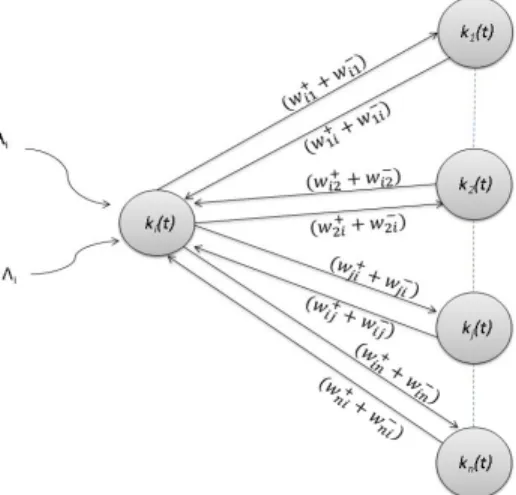
In the RNN (shown in Figure 2), signal travels in the form of impulses between the neurons. If the receiving signal has positive potential (+1) it represents excitation, and if the potential of the input signal is negative (-1) it represents
inhibition to the receiving neuron. Each neuron iin the RNN has a stateki(t) which represents the potential at time
t. This potential ki(t) is represented by a non-negative integer. If ki(t)>0 then neuron i is in excited state and if
ki(t) = 0 then neuron iis in idle state.
When neuron i is in excited state, it transmits an impulse according to the Poisson process rate ri. The transmitted
signal can reach neuron j as an excitation signal with probability p+(i, j) or as inhibitory signal with probability
p−(i, j), or it can leave the network with probabilityd(i) such that for alli,
d(i) + N X j=1 p+(i, j) +p−(i, j) = 1, w+(i, j) =rip+(i, j)>0, w−(i, j) =rip−(i, j)>0, (1) so that r(i) = (1−d(i))−1 N X j=1 w+(i, j) +w−(i, j), (2)
FIGURE2. Schematic Representation of Neurons in a Random Neural Network
TABLE 2. Description of RNN symbols
RNN Symbols Description
qi Probability neuroniexcited at timet
p+(i, j) Probability neuronjreceives positive signal from neuroni
p−(i, j) Probability neuronjreceives negative signal from neuroni
ri Firing rate of neuroni
Λi Arrival rate of external positive signals λi Arrival rate of external negative signals
d(i) Probability a signal from neuron departs from the network
ki(t) Potential of neuroniat timet
which is the firing rate of neuron i. Since the ’w’matrices are the product of firing rates and probabilities, they are
always non-negative. External excitatory and inhibitory signals can also reach neuroniaccording to Poisson processes
of rate Λi and λi, respectively. When an exciitory spike or positive is received at neuron i its potential ki(t) will
increase to +1. If neuron i is excitated and it receives an inhibitory spike, the potential of neuron iwill decrease to
zero. Arrivals of inhibitory or negative signals will have no effect on neuron i if its potential is already zero. The
description of the symbols used are given in Table 2. Consider the vectorK(t)= (k1(t), ...kn(t))whereki(t)is the
potential of neuron iand n is the total number of neurons in the network. LetKis continuous time Markov process.
The stationary distribution of K is represented by:
lim t→∞P r(K(t))) = (k1(t)...kn(t)) = n Y i=1 (1−qi)qnii , qi = G + i ri+G−i , (3) where G+i = Λi+ N X j=1 qjw+(j, i), G−i =λi+ N X j=1 qjw−(j, i). (4)
For a three layer network, the qi for each layer is calculated as:
qi = Λi ri+λi, qh= P iεIqiw+(i, h) rh+ P iqiw−(i, h) , qo = P iqhw+(h, o) rh+ P iqhw−(h, o) , (5)
when I, H and O denote the sets of Input, Hidden and Output layers, respectively, and i ∈ I, h ∈ H, o ∈ O.
According to Mohamed and Rubino [69], the cost of computing the output of the RNN is Θ(2|I||H|+ 3|H|+|I|)
products (or divisions) and Θ(|H|+|I|) sums, where |X|denotes the number of elements of set X. input neurons
4 LEARNING ALGORITHMS
A useful objective function for training the RNN given in (6) Gelenbe [30] is the quadratic cost function:
f(x) = 1 2 N X p=1 X o∈O [qo(p)−qdes,o]2, (6)
where N is the number of patterns, andqo(p) is the output of the RNN calculated by solving (5).
The GD algorithm developed by Gelenbe [30] adjusts the parameters in order to minimise the cost function f(x)
represented by Eq. (6). For details of updating the weights of RNN with GD algorithm, reader is referred to Gelenbe [30].
4.1 Artificial Bee Colony Algorithm
In this work, the ABC algorithm proposed in Karaboga and Basturk [65] was used for training the RNN. The ABC algorithm was used to find optimised weights of the RNN. The procedure for finding the optimal weights for the RNN using ABC algorithm is as follows:
Step1: Initialise a population of si solutions, where i = 1....SN, and SN denotes the size of population. Each
solution is D dimensional vector, whereDrepresents the number of parameters to be optimised. Each solution is an
array of interconnected weights of the feed forward RNN ofI Input nodes,H hidden nodes andOoutput nodes. The
dimensions of Dis 2(I.H+H.O). The solution (food source positions) is formulated assi = [w+ihL1who+L2wih−L1w−hoL2],
where i∈I, h∈H, o∈O. The weights are randomly distributed over the interval of [0,1].
wih+L1 is positive interconnection weight between node iof layer 0 and node h of layer 1.
who+L2 is positive interconnection weight between node h of layer 1 and node o of layer 2.
wih−L1 is negative interconnection weight between node iof layer 0 and node h of layer 1.
who−L2 is negative interconnection weight between node h of layer 1 and node o of layer 2.
Step-2: Evaluate the fitness value (f iti) of population (see Karaboga and Basturk [65]).
where f iti = 1 1+f(x) if f(x)>0 1 +|(f(x)| if f(x) <0 (7)
Step-3: For each employed bee, calculate new solution Vij and evaluate the fitness.
Vij =sij +θij(sij−skj) (8)
where k= 1,2, ....SN, andj= 1,2, ...., D are randomly chosen indexes, andθij is a random number between [-1,
1]. θij controls the contribution of difference of two randomly selected positions in production of neighbour food
sources are sij.
Step4: Apply the greedy selection process.
Step5: Calculate the probability value P robi of the solution si by using Eq. (9).
P robi =
f iti
PSN
n=1f iti
(9)
Step6: For each onlooker bee, calculate the new solutionVij by selecting the solution sij on the basis of probability
P robij.
Step7: Calculate the fitness value f iti.
Step8: Apply the greedy selection process.
Step9: Check if there is any food source abandoned by the bees. If there is any scout bee will randomly determine
the new food source (solution si) by using Eq. (10).
sij =sjmin+rand(0,1)(sjmax−s j
minf(x) = 2 p=1o=1 [qo(p)−qdes,o] (11) subject to c(x) = 0 (12)
where 06 X 61, N is the number of patterns, O is the number of output, qdes,o is the desired output in training
pattern, qo(p) is the output of RNN calculated by solving Eq. (5).
Constraint handling strategies usually convert the problem into sub-problems so that it can be easily solved, and used as the basis of an iterative process. In de Freitas Vaz and da Grac¸a Pinto Fernandes [24], Venter and Haftka [78], Richards [73], the constraint problems are transformed into unconstrained problems. The constraint handling strategies should preserve the feasibility of constraints in the optimisation solution. This constraint feasibility can be guaranteed by including Karush-Kuhn Tucker (KKT) equations in optimisation formulation. The KKT equations are necessary and sufficient condition for optimality of constrained optimisation problem.
SQP proposed in Hock and Schittkowski [55] is an efficient and accurate non linear programming method for constrained optimisation. The SQP algorithm can be considered as an application of Newton’s method to Karush-Kuhn Tucker (KKT) optimality conditions for Eq. (6). The SQP uses BFGS quasi newton method to calculate the approximation of Hessian of Lagrangian function at every iteration.The problem is transformed in to quadratic programming (QP) sub-problem stated whose solution is used to form a search direction for a line search procedure.
The Lagrangian function is shown in Eq. (13) where λis the vector of Lagrangian multiplier
L(Xk, λ) =f(Xk) +c(Xk)Tλ (13)
The problem is transformed in to quadratic programming (QP) sub-problem stated by Eq. (11) subject to Eq. (12)
min1
2d
TH
kd+5f(Xk)Td (14)
subject to Lb6Xk+dk6U b
The Hessian of the Lagrangian function is constructed from quasi newton formula
Hk+1=Hk+ qkqkT qTksk −H T ksTkskHk sTkHksk (15) where sk=Xk+1−Xk (16) qk =5L(Xk+1, λk+1)− 5L(Xk, λk+1) (17)
At every iteration of QP sub-problem, the direction dk is obtained using Eq. (14). The new iterate obtained by using
this solution is given by
Xk+1 =Xk+αkdk (18)
where αkis the step length values used to obtain sufficient decrease in augmented Lagrangian function
LA(X, λ, ρ) =f(X)−λT(X) + ρ
2c(X)C(X) (19)
ρ is non-negative scalar. The procedure will continue until the minimum threshold of Eq. (11) is achieved or sk has
Initialize the random neural network with random interconnected weights sij =[wij+L1 wij+L2 wij-L1 wij-L2 ]
Train the network with ABC algorithm
If ABC training finished
NO
Store the weights YES
Train the network with SQP optimization algorithm
If training finished
NO
Store the weights YES
FIGURE3. The flow diagram of hybrid ABC-SQP algorithm
4.3 Hybrid Artificial Bee Colony Algorithm with Sequential Quadratic Programming Algorithm
The ABC algorithm is good in finding global minima but it might be slow to converge to global minima, while in presence of multiple local minima, SQP optimisation method usually converges to local minima. In this paper, we propose a hybrid ABC-SQP algorithm for RNN training. First, RNN was trained with ABC algorithm to find the global minima, then based on this feasible start point from ABC algorithm, SQP optimisation algorithm converged to global minima. The flow chart of the hybrid ABC-SQP is shown in Figure 3.
4.4 Particle Swarm Optimisation for Training RNN
4.4.1 AIW-PSO Learning Procedure
The steps required for the implementation of AIW-PSO training algorithm proposed in Georgiopoulos et al. [52] are as follows:
Step1: Initialise a population of S particles with random positions and velocities of d dimensions in the problem
space. The position vector is an array of interconnected weights of feed forward RNN of I Input nodes, H hidden
nodes and O output nodes. The dimensions of D is 2(I.H+H.O). The position vector is formulated as Xsd =
[w+ihL1who+L2wih−L1w−hoL2], where i ∈ I, h ∈ H, o ∈ O. The weights are randomly distributed over the interval of
[0,1].
Step2: Each particle from position in generation k moves to new position k+1by using PSO equation given in Eq.
(20). The c1 constant value is set to 2.6 andc2, constant value is set to 1.1.
Vsdk+1=W Vsdk +c1rand()(Pbestsdk −Xsdk) +c2rand()(Gkbestsd−Xsdk) (20) Xsdk+1=Xsdk +Vsdk+1 (21) Wsdk = 1− 1 1 +exp(−α.ISAk sd) (22) ISAksd= Xsdk −Pbestsdk Pbestsdk −Gkbestsd (23)
Store the weights
YES
Train the network with SQP optimization algorithm
If training finished NO
Store the weights
YES
FIGURE4. The flow diagram of hybrid PSO-SQP algorithm
Step3: For each particle, evaluate the fitness function of Eq. (6).
Step4: Compare particle fitness evaluation with particle’s personal best Pbest. If current fitness evaluation value is
less than Pbest, then update Pbest to current value and thePbest location equal to current location in Ddimensional
space.
Step5: Compare fitness evaluation with allPbestof populationS. IfPbestis less thanGbestupdateGbestto the current
particle’s array index.
Step6: For checking the convergence criteria, compute the average squared error of Eq. (6). If the MSE is not less than threshold, go to Step 2. If stopping criteria for maximum number of iterations is achieved, learning is complete.
4.5 Hybrid Particle Swarm Optimisation with Sequential Quadratic Programming
The hybrid PSO-SQP algorithm first uses the PSO algorithm for finding the global minima, then based on this feasible start point from ABC algorithm, SQP optimisation algorithm converged to global minima. In this paper, the number of iterations for PSO is set to 2000. After getting initial starting point from PSO the SQP optimisation algorithm has been executed for maximum of 400 iterations. The flow chart of PSO-SQP is shown in Figure 4.
4.6 Differential Evolution Optimisation for Training RNN
The steps required for the implementation of DE training algorithm proposed in Georgiopoulos et al. [52] are as follows:
Step1: Initialise a population of S particles with random positions and velocities of D dimensions in the problem
space. The position vector is an array of interconnected weights of feed forward RNN of I Input nodes, H hidden
nodes and O output nodes. The dimensions of D is 2(I.H+H.O). The position vector is formulated as Xsd =
[w+ihL1who+L2wih−L1who−L2], where L1 is the layer 1, L2 is the layer 2, and i ∈ I, h ∈ H, o ∈ O. The weights are
randomly distributed over the interval of [0,1].
Step2: Randomly generate three integer numbers r1d, r2d, r3d[1, S], wherer1d6=r2d6=r3d6=S. Set the value of F
and CR to 0.8 and 0.7 respectively.
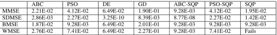
TABLE 3. Statistical Results for XOR problem with ABC, PSO, DE, GD, ABC-SQP, PSO-SQP, SQP
ABC PSO DE GD ABC-SQP PSO-SQP SQP
MMSE 2.21E-02 4.12E-02 6.49E-02 1.90E-01 9.28E-03 4.12E-02 1.95E-02
SDMSE 2.86E-03 2.27E-02 3.25E-10 8.39E-03 8.77E-08 2.27E-02 1.42E-02
BMSE 1.87E-02 9.28E-03 6.49E-02 2.01E-01 9.28E-03 9.28E-03 9.28E-03
WMSE 2.76E-02 7.41E-02 6.49E-02 2.27E-01 9.28E-03 7.41E-02 Fails
different from other Evolutionary algorithms. Mutate every particle of the population (16s6S) by applying the
DE equation
Ysdk+1=Xrk1d+F(Xr2d−Xr3d) (24)
The mutated sth particle at generation k+1is of dimensionD. The mutated sth particle is sum of another particle at
location r1d and difference of particle values at location r2d and r3d. The contribution of difference of particles is
controlled by parameter F.
Step4: Randomly generate one real number rand()[0,1]. Cross over the mutated particle and the original particle
using the Eq. (25).
Usdk+1=Ysdk+1 if rand()6CR Usdk+1=Xsdk+1 if rand()> CR
(25)
Step5: Evaluate the fitness function given in Eq. (6) forUsdk+1. If fitness value forUsdk+1 is less thanXsdk, then update
Xsdk+1 toUsdk+1 elseXsdk+1 =Xsdk.
Step6: For checking the convergence criteria, compute the average squared error of Eq. (6). If the mean square error is not less than threshold, go to Step2. If stopping criteria is met or maximum number of iterations is achieved, learning is complete.
5 RESULTS
In this section, the performance of the algorithms are compared for six different test problems. Problem 1, Problem 2 and Problem 3 are examples of pattern classification while Problem 4, Problem 5 and Problem 6, Problem 7 are examples of function approximations. The mean of MSE (MMSE), Standard Deviation of MSE (SDMSE), Best Mean Squared Error (BMSE) and Worst Mean Squared Error (WMSE) were compared for different number of iterations. The performance of algorithms were further compared in terms of NRMSE and computational time.
The learning rate for the GD algorithm was 0.01. Population size for ABC, PSO, SQP was 40. The maximum number of iteration/epochs for GD/ABC/PSO/DE algorithms was 2000.
5.1 Comparison of Training Algorithms for Pattern Classification Problems
5.1.1. Test Problem 1- XOR Problem
The exclusive-OR (XOR) problem has been widely used by researchers for evaluating the performance of learning algorithms. The XOR is difficult classification problem of mapping two binary numbers into one binary output. In this evaluation, a 2-4-1 feed forward network with 24 interconnection weights was used for comparison. The inputs and
outputs are normalised between 0 and 1. The value of Dwas 24, whereDis the number of optimisation parameters.
The MMSE, SDMSE, BMSE, and WMSE for XOR problem in relation to ABC, PSO, DE, GD, ABC-SQP, PSO-SQP and SQP are given in Table 3. The MMSE achieved by the GD algorithm was 1.90E-01, while the MMSE achieved by ABC was 2.21E-02, 4.12E-02 with the PSO, 6.49E-02 with DE after 2000 iterations. The MMSE achieved by ABC-SQP was 9.28E-03, 4.12E-02 with PSO-SQP and 1.92E-02 with SQP.
The hybrid ABC algorithm outperformed all algorithms and the MMSE was 9.28E-03 after 100 iterations. The MMSE of ABC-SQP algorithm was 95.16% less than GD algorithm while the MMSE of ABC-SQP was 77.42% less than the PSO/PSO-SQP algorithm, 85.7% less than the DE, 52.4% less than the SQP, 57.8% less than the ABC and 95.16% less than the GD algorithm. The BMSE achieved by ABC-SQP, PSO-SQP and SQP was 9.28E-03 but PSO-SQP and SQP was not robust, and in case of SQP the failure rate (the SQP failed to start) was 40%.
x y z f(x,y,z) 0 0 0 0 0 0 1 1 0 1 0 1 0 1 1 0 1 0 0 1 1 0 1 0 1 1 0 0 1 1 1 1
5.1.2. Test Problem 2- Parity Bit Problem
The RNN learning algorithms were also tested against parity bit problem. A 3-4-1 feedforward RNN network with 32 interconnection weights was trained. If the number of binary inputs were odd, the output was 1 otherwise output was 0 as shown in Table 5. The inputs for RNN were x, y, z, and the output of RNN was f(x,y,z). The MMSE, SD-MSE, WMSE and BMSE with the GD, ABC, PSO, DE, ABC-SQP, PSO-SQP and SQP are shown in Table 4. The MMSE with ABC algorithm was 1.11E-01, with PSO was 1.40E-01, with DE was 1.21E-01, with GD was 2.22E-01, with ABC-SQP was 1.03E-01, with PSO-SQP was 1.38E-01 and with SQP was 1.16E-01. Results showed that the ABC-SQP algorithm outperformed other algorithms. The MMSE with ABC-SQP was 54.5% less than GD, 15.5% less than DE, 26.9% less than PSO, 7.74% less than ABC, 25.83% less than PSO-SQP, and 11.1% less than SQP. The failure rate of SQP algorithm was 28.75%.
5.1.3. Test Problem 3- IRIS Flower Database
Iris dataset is one of the best known datasets available for pattern recognition problems and is available in Bache and Lichman [8]. The data set contains 3 classes (Iris Setosa, Iris Versicolour, Iris Virginica) of 50 instances each, in which each class refers to a type of Iris plant. The inputs for the dataset were: Sepal length in cm, Sepal width in cm, Petal length in cm, Petal width in cm. For classification, a feed forward RNN with 5 neurons in hidden layer gave good performance. The mean percentage of correct classification after 10 runs with GD algorithm was 66.7%, with ABC was 87.3% with ABC-SQP was 95.33%, with PSO was 68.21%, with PSO-SQP was 95.10%, with SQP was 95.10%, with DE was 86.78%.
5.2 Comparison of training algorithms for Function Approximation Problems
5.2.1. Test Problem 4- Temperature Prediction for residential building
The training algorithms were compared for training a RNN model used for building energy usage described in Javed et al. [60]. The future air temperature of the living room was predicted by the RNN model which was three layered network and trained with data of 05 days collected after every 120 seconds from living room of the building and
validated with data of 15 days. During the training period the outside temperature varied between -8.2 ◦C to 7.7 ◦C
and during the validation period the outside temperature varied between -21.1 ◦C to 10.3 ◦C. The RNN model had
four neurons as input layer, five neurons in the hidden layer and 1 neuron in the output layer. The inputs of the RNN
model were current room air temperature (Tair), outside temperature (Tout), the number of occupants and flowrate
(m0) of inlet water for radiator, and the output of the RNN model was the future (t+2 minutes) air temperature of
room at present time 0t0. The input data was normalised between 0.1 and 0.9.
A 4-5-1 feedforward RNN model with 50 interconnection weights was trained. The MMSE, SDMSE, BMSE, and WMSE for the temperature forecast problem with ABC, PSO, DE, GD, ABC-SQP, PSO-SQP, and SQP are given in
TABLE 6. Statistical Results for Temperature forecast problem with ABC, PSO, DE, GD, ABC-SQP, PSO-SQP, SQP
ABC PSO DE GD ABC-SQP PSO-SQP SQP
MMSE 2.77E-04 8.33E-04 3.56E-05 2.52E-03 1.28E-06 1.28E-06 1.30E-06
SDMSE 1.08E-04 8.46E-04 4.69E-05 5.23E-04 1.02E-08 9.10E-10 5.19E-08
BMSE 1.52E-04 1.31E-06 1.30E-06 1.74E-03 1.26E-06 1.28E-06 1.28E-06
WMSE 4.38E-04 2.09E-03 1.28E-04 8.46E-04 1.29E-06 1.29E-06 1.45E-06
TABLE 7. Statistical Results for Temperature forecast problem for three zone building with ABC, PSO, DE, GD, ABC-SQP, PSO-SQP, SQP
ABC PSO DE GD ABC-SQP PSO-SQP SQP
MMSE 9.88E-03 2.40E-02 9.58E-03 5.36E-02 3.89E-03 5.48E-03 4.00E-03
SDMSE 7.36E-04 4.17E-03 9.37E-04 6.92E-03 1.51E-04 1.64E-03 6.97E-05
BMSE 9.02E-03 1.73E-02 7.98E-03 4.09E-02 3.57E-03 3.68E-03 3.89E-03
WMSE 1.12E-02 2.98E-02 1.07E-02 6.28E-02 4.04E-03 7.77E-03 4.10E-03
Table 6. After 2000 iterations the MMSE achieved with ABC algorithm was 2.77E-04, with PSO was 8.33E-04, with DE was 3.56E-05, with GD was 2.52E-03. The MMSE after 250 iterations with ABC-SQP algorithm was 1.27E-06, with PSO-SQP was 1.28E-06 and with SQP was 1.30E-06. The MMSE for ABC-SQP algorithm was 99.53% less than ABC-algorithm, 99.85% less than PSO, 96.40% less than DE, 99.94% less than GD, 0.38% less than PSO-SQP and 1.61% less than SQP algorithm.
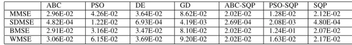
5.2.2. Test Problem 5- Three Zone Building Model
A three zone single storey building situated in Chicago, USA was modelled in Energy Plus to generate training dataset for system identification using MLE+ (see Bernal et al. [12]). The building was fitted with floor heating system. The inputs for the RNN model were: temperature setpoint for zone 1, temperature setpoint for zone 2, temperature setpoint for zone 3, outside temperature, transmitted solar gains, total internal heat gains in zone 1, total internal heat gains in zone 2, total internal heat gains in zone 3, and floor temperature. The outputs of the RNN model were mean air temperature for zone 1, mean air temperature for zone 2, and mean air temperature for zone 3. A RNN model with 9 neurons in the hidden layer gave the best performance so the selected RNN model was 9-9-3 network. The statistical results with ABC, PSO, DE, GD ABC-SQP, PSO-SQP and SQP for this problem are given in Table 7. The MMSE with ABC-SQP algorithm was 60.7% less than ABC algorithm, 83.76% less than PSO, 59.49% less than DE, 92.75% less than GD, 29.06% less than PSO-SQP and 3.02% less than SQP algorithm.
5.2.3. Test Problem 6- Engine Behaviour Modelling
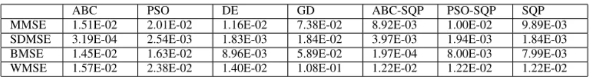
This dataset was collected during an engine operation and available with neural network toolbox (see Beale et al. [11]). This benchmark problem is an example of nonlinear regression or function approximation problem. The engine speed and fuel rate are selected as inputs to the network while engine torque and nitrous oxide emission were selected as network outputs. A 2-4-2 RNN was selected for this problem. The statistical results of ABC, PSO, DE, GD, ABC-SQP, PSO-SQP and SQP are given in Table 8. The MMSE with ABC-SQP algorithm was 42.20% less than ABC algorithm, 55.5% less than PSO, 22.6% less than DE, 64.4% less than GD, 11.17% less than PSO-SQP and 10.01% less than SQP algorithm.
TABLE 8. Statistical Results for Engine Behaviour problem with ABC, PSO, DE, GD, ABC-SQP, PSO-SQP, SQP
ABC PSO DE GD ABC-SQP PSO-SQP SQP
MMSE 1.51E-02 2.01E-02 1.16E-02 7.38E-02 8.92E-03 1.00E-02 9.89E-03
SDMSE 3.19E-04 2.54E-03 1.83E-03 1.84E-02 3.97E-03 1.94E-03 1.84E-03
BMSE 1.45E-02 1.63E-02 8.96E-03 5.89E-02 1.97E-04 8.00E-03 7.99E-03
Problem ABC PSO DE GD ABC-SQP PSO-SQP SQP Problem 1 70.16% 61.50% 49.29% 50.29% 80.76% 61.5% 73.95 Problem 2 33.63% 25.23% 30.60 % 2.24% 36.31% 25.84% 36.29% Problem 4 90.04% 84.13% 96.97% 66.67% 99.31% 99.31% 99.31% Problem 5 79.32% 67.45% 79.82% 77.31% 87.16% 84.88% 86.96% Problem 6 72.29% 67.56% 75.65% 54.27% 77.88% 78.00% 77.72 % Problem 7 47.94% 37.20% 40.2% 8.95% 59.02% 58.45% 60.86 %
5.2.4. Test Problem 7- Occupancy Estimation
We exploited the significant statistical correlations between the occupancy levels and the CO2 concentration, room
temperature, and ventilation actuation signals in order to identify a dynamic model for estimation of the occupancy level in Javed et al. [63]. The inputs for the RNN model were: air temperature of room, inlet air temperature, inlet
CO2 concentration, indoor CO2 levels, and inlet air actuation signal while output of RNN model is occupancy levels.
The statistical results of ABC, PSO, DE, GD, ABC-SQP, PSO-SQP and SQP are given in Table 9.
5.3 Performance comparison for Normalised room mean square error
The validation metric used in this work is fitness value (i.e.,NRMSE) defined in the system identification toolbox of Matlab as follows f it:= 1− kyˆ−yk y− 1 N Pi=1 N y(i) ×100 (26)
where yˆ is output of RNN andy is the target output. The fitness percentage for all test problems are given in Table
10. The ABC-SQP outperformed other algorithms for all problems in terms of NRMSE. Results showed that the ABC-SQP problem outperformed other training algorithms in terms of fitness percentage except for Problem 6 and Problem 7. For Problem 6, the fitness percentage of PSO-SQP is 78% which is 0.12% better than ABC-SQP. Similarly for Problem 7, the fitness percentage of SQP is 1.84% better than ABC-SQP.
5.4 Comparison of computational time
The computational time required by training algorithms was also compared for all test problems as shown in Table 11 in terms of average execution time required for each iteration. The average execution time by GD for all problems was the lowest but the MMSE for the GD algorithm was highest. The execution time by ABC, DE, and PSO was dependent on size of population, greater the population size higher is the execution time.
TABLE 11. Average computational time - Iteration per seconds
Problems ABC PSO DE GD ABC-SQP PSO-SQP SQP
Problem 1 0.024 0.029 0.549 0.0086 0.020 0.029 0.0189 Problem 2 0.030 0.036 0.92 0.011 0.030 0.036 0.038 Problem 3 0.39 0.4 0.63 0.135 0.41 0.44 0.76 Problem 4 8.39 8.66 12.57 3.21 9.13 8.68 9.05 Problem 5 2.62 2.76 15.52 3.19 6.38 6.55 30.48 Problem 6 2.44 1.56 4.06 0.90 2.56 1.64 2.74 Problem 7 0.62 0.59 1.16 0.47 0.74 0.77 2.02
6 CONCLUSION
In this work, the ABC algorithm which is a relatively new algorithm for optimisation has been used for training RNN models for pattern classification problems (Problem 1, Problem 2, Problem 3) and function approximation problems (Problem 4, Problem 5, Problem 6, Problem 7). A hybrid ABC-SQP algorithm has also been proposed in this study which was developed by combining the ABC algorithm and the SQP optimisation algorithm. The ABC-SQP combined the strength of ABC algorithm for finding global minima and strength of ABC-SQP optimisation algorithm for convergence to minima based on feasible starting point. The results of this work showed that ABC and ABC-SQP can successfully be used for training RNN models and ABC-SQP algorithm outperformed ABC, PSO, PSO-SQP, DE and GD algorithm in terms of MSE and NRMSE.
For function approximation problems i.e., Problem 4, Problem 5, Problem 6, and Problem 7, the performance of the DE algorithm was better than the ABC algorithm in terms of NRMSE, and MMSE. However, the computational time of ABC was 33.25% less than DE for Problem 4, 83.11% less than DE for Problem 5, 39.9% less for Problem 6 and 54% less for Problem 7. Due to the higher execution time, the DE was not suitable for hybridisation with SQP algorithm. The execution time of the GD algorithm for training Problems 1-7 was 57.5%, 63.33% 67.07%, 64.8%, 50.0% and 64.84% respectively less than the execution time required by the ABC-SQP algorithm.
However, the MMSE of the ABC-SQP algorithm was 95.16 % less than GD for Problem 1, 54.5% less for Problem 2, 99.94% less for Problem 4, 92.75% less for Problem 5, 64.4% less than GD for Problem 6 and 57.4% less than GD for Problem 7. It was further noticed that the ABC algorithm outperformed the GD algorithm in terms of MSE and NRMSE.
In the majority of the function approximation and pattern classification problems, the accuracy of the trained network was more important than the computational time that was being used. By minor compromises on computational time, the training error could be reduced significantly. In real time applications, the training algorithm needs to be be robust and accurate, and the results showed that the ABC and ABC-SQP algorithms were more robust and accurate than other algorithms.
REFERENCES
[1] Abdelbaki, H. (1999). Random neural network simulator (rnnsim) v. 2. Free simulator available at ftp://ftp.
mathworks. com/pub/contrib/v5/nnet/rnnsimv2, .
[2] Abdelbaki, H., Gelenbe, E., and El-Khamy, S. E. (2000). Analog hardware implementation of the random neural
network model. In Proceedings of the IEEE-INNS-ENNS International Joint Conference on Neural Networks,
2000. IJCNN 2000 (pp. 197–201). IEEE volume 4.
[3] Abdelbaki, H., Gelenbe, E., and Kocak, T. (2005). Neural algorithms and energy measures for emi based mine
detection. Differential Equations and Dynamical Systems, 13, 63–86.
[4] Abdelrahman, O. H., and Gelenbe, E. (2015). Search in big networks and big data. In Analytic Methods in
Interdisciplinary Applications (pp. 1–15). Springer International Publishing.
[5] Aguilar, J., and Colmenares, A. (1998). Resolution of pattern recognition problems using a hybrid genetic/random
neural network learning algorithm. Pattern Analysis and Applications, 1, 52–61.
[6] Akinwande, O. J., Bi, H., and Gelenbe, E. (2015). Managing crowds in hazards with dynamic grouping. IEEE
Access, 3, 1060–1070.
[7] Atalay, V. (1998). Learning by optimization in random neural networks. In Proceedings of the Thirteenth
International Symposium on Computer and Information Sciences, Antalya, Turkey (pp. 143–148).
[8] Bache, K., and Lichman, M. (2013). UCI machine learning repository. URL:
http://archive.ics.uci.edu/ml.
[9] Bakirciouglu, H., Gelenbe, E., and Kocak, T. (1997). Image enhacement and fusion with the random neural
network. Turkish Journal Of Electrical Engineering & Computer Sciences, 5, 65–77.
[10] Basterrech, S., Mohammed, S., Rubino, G., and Soliman, M. (2011). Levenbergmarquardt training algorithms
for random neural networks. The Computer Journal, 54, 125–135.
[11] Beale, M. H., Hagan, M. T., and Demuth, H. B. (2010). Neural network toolbox 7. Users Guide, MathWorks, .
[12] Bernal, W., Behl, M., Nghiem, T. X., and Mangharam, R. (2012). Mle+: a tool for integrated design and
deployment of energy efficient building controls. In Proceedings of the Fourth ACM Workshop on Embedded
[16] Cancela, H., Robledo, F., and Rubino, G. (2004). A grasp algorithm with rnn based local search for designing
a wan access network. Electronic Notes in Discrete Mathematics, 18, 59–65.
[17] Ceran, E. T., and Gelenbe, E. (2016). Energy packet model optimisation with approximate matrix inversion. In
Proceedings of the 2nd International Workshop on Energy-Aware Simulation (p. 4). ACM.
[18] Cerkez, C., Aybay, I., and Halici, U. (1997). A digital neuron realization for the random neural network model. InInternational Conference on Neural Networks, 1997. (pp. 1000–1004). IEEE volume 2.
[19] Chau, K. (2006). Particle swarm optimization training algorithm for anns in stage prediction of shing mun river.
Journal of hydrology, 329, 363–367.
[20] Cramer, C., Gelenbe, E., and Bakircloglu, H. (1996). Low bit-rate video compression with neural networks and
temporal subsampling. Proceedings of the IEEE,84, 1529–1543.
[21] Eberhart, R. C., and Kennedy, J. (1995). A new optimizer using particle swarm theory. In Proceedings of the
sixth international symposium on micro machine and human science (pp. 39–43). New York, NY volume 1. [22] Fourneau, J.-M., Gelenbe, E., and Suros, R. (1996). G-networks with multiple classes of negative and positive
customers. Theoretical Computer Science, 155, 141–156.
[23] Francois, F., and Gelenbe, E. (2016). Towards a cognitive routing engine for software defined networks. In
Communications (ICC), 2016 IEEE International Conference on (pp. 1–6). IEEE.
[24] de Freitas Vaz, A. I., and da Grac¸a Pinto Fernandes, E. M. (2006). Optimization of nonlinear constrained particle
swarm. Technological and Economic Development of Economy, 12, 30–36.
[25] Garro, B. A., Sossa, H., and V´azquez, R. A. (2011). Artificial neural network synthesis by means of artificial
bee colony (abc) algorithm. In2011 IEEE Congress on Evolutionary Computation (CEC)(pp. 331–338). IEEE.
[26] Gelenbe, E. (1989). Random neural networks with negative and positive signals and product form solution.
Neural computation, 1, 502–510.
[27] Gelenbe, E. (1990). Stability of the random neural network model. Neural computation, 2, 239–247.
[28] Gelenbe, E. (1991). Product-form queueing networks with negative and positive customers. Journal of Applied
Probability, (pp. 656–663).
[29] Gelenbe, E. (1993). G-networks with triggered customer movement. Journal of Applied Probability, (pp.
742–748).
[30] Gelenbe, E. (1993). Learning in the recurrent random neural network. Neural Computation, 5, 154–164.
[31] Gelenbe, E. (1994). G-networks: a unifying model for neural and queueing networks. Annals of Operations
Research, 48, 433–461.
[32] Gelenbe, E. (2000). The first decade of g-networks. European Journal of Operational Research, 126, 231–232.
[33] Gelenbe, E. (2014). Error and energy when communicating with spins. In Signal and Information Processing
(GlobalSIP), 2014 IEEE Global Conference on (pp. 784–787). IEEE.
[34] Gelenbe, E. (2015). Errors and power when communicating with spins. IEEE Transactions on Emerging Topics
in Computing, 3, 483–488.
[35] Gelenbe, E. (2015). Synchronising energy harvesting and data packets in a wireless sensor.Energies,8, 356–369.
[36] Gelenbe, E. (2016). Agreement in spins and social networks. ACM SIGMETRICS Performance Evaluation
Review, 44, 15–17.
[37] Gelenbe, E., and Ceran, E. T. (2015). Central or distributed energy storage for processors with energy harvesting. InSustainable Internet and ICT for Sustainability (SustainIT), 2015 (pp. 1–3). IEEE.
[38] Gelenbe, E., and Ceran, E. T. (2016). Energy packet networks with energy harvesting. IEEE Access, 4, 1321–
1331.
[39] Gelenbe, E., Feng, Y., and Krishnan, K. R. R. (1996). Neural network methods for volumetric magnetic resonance
[40] Gelenbe, E., and Fourneau, J.-M. (2002). G-networks with resets. Performance Evaluation,49, 179–191.
[41] Gelenbe, E., Hussain, K., and Kaptan, V. (2005). Simulating autonomous agents in augmented reality. Journal
of Systems and Software, 74, 255–268.
[42] Gelenbe, E., and Hussain, K. F. (2002). Learning in the multiple class random neural network.IEEE Transactions
on Neural Networks,13, 1257–1267.
[43] Gelenbe, E., and Kazhmaganbetova, Z. (2014). Cognitive packet network for bilateral asymmetric connections.
IEEE Transactions on Industrial Informatics, 10, 1717–1725.
[44] Gelenbe, E., and Labed, A. (1998). G-networks with multiple classes of signals and positive customers. European
journal of operational research, 108, 293–305.
[45] Gelenbe, E., and Marin, A. (2015). Interconnected wireless sensors with energy harvesting. In International
Conference on Analytical and Stochastic Modeling Techniques and Applications (pp. 87–99). Springer International Publishing.
[46] Gelenbe, E., and Schassberger, R. (1992). Stability of product form g-networks. Probability in the Engineering
and Informational Sciences, 6, 271–276.
[47] Gelenbe, E., and Shachnai, H. (2000). On g-networks and resource allocation in multimedia systems. European
Journal of Operational Research, 126, 308–318.
[48] Gelenbe, E., and Timotheou, S. (2008). Synchronized interactions in spiked neuronal networks. The Computer
Journal, 51, 723–730.
[49] Gelenbe, E., and Wang, L. (2016). Tap: A task allocation platform for the eu fp7 panacea project. InAdvances in
Service-Oriented and Cloud Computing: Workshops of ESOCC 2015, Taormina, Italy, September 15-17, 2015, Revised Selected Papers (p. 425). Springer volume 567.
[50] Gelenbe, E., and Wu, F.-J. (2012). Large scale simulation for human evacuation and rescue. Computers &
Mathematics with Applications, 64, 3869–3880.
[51] Gelenbe, E., and Yin, Y. (2016). Deep learning with random neural networks. In 2016 International Joint
Conference on Neural Networks (IJCNN) (pp. 1633–1638). IEEE.
[52] Georgiopoulos, M., Li, C., and Kocak, T. (2011). Learning in the feed-forward random neural network: A
critical review. Performance Evaluation, 68, 361–384.
[53] Halici, U. (1997). Reinforcement learning in random neural networks for cascaded decisions. Biosystems, 40,
83–91.
[54] Henderson, W. (1993). Queueing networks with negative customers and negative queue lengths. Journal of
Applied Probability, (pp. 931–942).
[55] Hock, W., and Schittkowski, K. (1983). A comparative performance evaluation of 27 nonlinear programming
codes. Computing, 30, 335–358.
[56] Holland, J. H. (1975). Adaptation in natural and artificial systems: An introductory analysis with applications
to biology, control, and artificial intelligence.. U Michigan Press.
[57] Hubert, C. (1993). Pattern completion with the random neural network using the rprop learning algorithm. In Conference Proceedings., International Conference on Systems, Man and Cybernetics, 1993.’Systems Engineering in the Service of Humans’, (pp. 613–617). IEEE.
[58] Ilonen, J., Kamarainen, J.-K., and Lampinen, J. (2003). Differential evolution training algorithm for feed-forward
neural networks. Neural Processing Letters, 17, 93–105.
[59] Irani, R., and Nasimi, R. (2011). Application of artificial bee colony-based neural network in bottom hole
pressure prediction in underbalanced drilling. Journal of Petroleum Science and Engineering, 78, 6–12.
[60] Javed, A., Larijani, H., Ahmadinia, A., and Emmanuel, R. (2014). Modelling and optimization of residential
heating system using random neural networks. In2014 IEEE International Conference on Control Science and
Systems Engineering (CCSSE) (pp. 90–95). IEEE.
[61] Javed, A., Larijani, H., Ahmadinia, A., Emmanuel, R., Gibson, D., and Clark, C. (2015). Experimental testing
of a random neural network smart controller using a single zone test chamber. IET Networks, 4, 350–358.
[62] Javed, A., Larijani, H., Ahmadinia, A., Emmanuel, R., Mannion, M., and Gibson, D. (2016). Design and implementation of cloud enabled random neural network based decentralized smart controller with intelligent
sensor nodes for hvac. IEEE Internet of Things Journal, PP, 1–1.
[63] Javed, A., Larijani, H., Ahmadinia, A., and Gibson, D. (2017). Smart random neural network controller
European Journal of Operational Research, 126, 331–339.
[68] Lu, R., and Shen, Y. (2006). Image segmentation based on random neural network model and gabor filters. In
27th Annual International Conference of the Engineering in Medicine and Biology Society, 2005. IEEE-EMBS 2005. (pp. 6464–6467). IEEE.
[69] Mohamed, S., and Rubino, G. (2002). A study of real-time packet video quality using random neural networks.
IEEE Transactions on Circuits and Systems for Video Technology, 12, 1071–1083.
[70] ¨Oke, G., and Loukas, G. (2007). A denial of service detector based on maximum likelihood detection and the
random neural network. The Computer Journal, 50, 717–727.
[71] Ozturk, C., and Karaboga, D. (2011). Hybrid artificial bee colony algorithm for neural network training. In
2011 IEEE Congress on Evolutionary Computation (CEC)(pp. 84–88). IEEE.
[72] Raja, M. A. Z., Samar, R. et al. (2014). Solution of the 2-dimensional bratu problem using neural network,
swarm intelligence and sequential quadratic programming. Neural Computing and Applications,25, 1723–1739.
[73] Richards, Z. D. (2009). Constrained particle swarm optimisation for sequential quadratic programming.
International Journal of Modelling, Identification and Control, 8, 361–367.
[74] Serrano, W., and Gelenbe, E. (2016). An intelligent internet search assistant based on the random neural network. InIFIP International Conference on Artificial Intelligence Applications and Innovations(pp. 141–153). Springer. [75] Shah, H., Ghazali, R., and Nawi, N. M. (2011). Using artificial bee colony algorithm for mlp training on
earthquake time series data prediction. Journal of Computing, 3, 135–142.
[76] Storn, R., and Price, K. (1997). Differential evolution–a simple and efficient heuristic for global optimization
over continuous spaces. Journal of global optimization, 11, 341–359.
[77] Timotheou, S. (2008). Nonnegative least squares learning for the random neural network. In Artificial Neural
Networks-ICANN 2008(pp. 195–204). Springer.
[78] Venter, G., and Haftka, R. (2010). Constrained particle swarm optimization using a bi-objective formulation.
Structural and Multidisciplinary Optimization, 40, 65–76.
[79] Wang, L., Brun, O., and Gelenbe, E. (2016). Adaptive Workload Distribution for Local and Remote Clouds. In
IEEE International Conference On Systems, Man, AND Cybernetics (SMC 2016). Budapest, Hungary.
[80] Wang, L., and Gelenbe, E. (2015). Adaptive dispatching of tasks in the cloud. IEEE Transactions on Cloud
Computing, PP, 1–1.
[81] Wang, L., and Gelenbe, E. (2015). Demonstrating voice over an autonomic network. In Autonomic Computing
(ICAC), 2015 IEEE International Conference on(pp. 139–140). IEEE.
[82] Wang, L., and Gelenbe, E. (2015). Experiments with smart workload allocation to cloud servers. In Network
Cloud Computing and Applications (NCCA), 2015 IEEE Fourth Symposium on(pp. 31–35). IEEE.
[83] Wang, L., and Gelenbe, E. (2016). Real-time traffic over the cognitive packet network. In International
Conference on Computer Networks (pp. 3–21). Springer International Publishing.
[84] Yin, Y., and Gelenbe, E. (2016). Deep learning in multi-layer architectures of dense nuclei. arXiv preprint
arXiv:1609.07160, .
[85] Zhang, J.-R., Zhang, J., Lok, T.-M., and Lyu, M. R. (2007). A hybrid particle swarm
optimization–back-propagation algorithm for feedforward neural network training. Applied Mathematics and Computation, 185,
1026–1037.
[86] Zhong, Y., Sun, D., and Wu, J. (2005). Dynamical random neural network approach to a problem of optimal