Computation and visualization of the MacAdam
limits for any lightness,
hue angle, and light source
Francisco Martínez-Verdú, Esther Perales, Elisabet Chorro, Dolores de Fez, and Valentín Viqueira Department of Optics, University of Alicante, Carretera de San Vicente del Raspeig s/n 03690,
Alicante, Spain Eduardo Gilabert
Department of Paper and Textile Engineering, Technical University of Valencia, Plaza de Ferrándiz y Carbonell, s/n 03801 Alcoy, Spain
Received March 14, 2006; revised November 23, 2006; accepted December 7, 2006; posted January 3, 2007 (Doc. ID 68782); published May 9, 2007
We present a systematic algorithm capable of searching for optimal colors for any lightnessL*(between 0 and
100), any illuminant (D65, F2, F7, F11, etc.), and any light source reported by CIE. Color solids are graphed in some color spaces (CIELAB, SVF, DIN99d, and CIECAM02) by horizontal (constant lightness) and transversal (constant hue angle) sections. Color solids plotted in DIN99d and CIECAM02 color spaces look more spherical or homogeneous than the ones plotted in CIELAB and SVF color spaces. Depending on the spectrum of the light source or illuminant, the shape of its color solid and its content (variety of distinguishable colors, with or without color correspondence) change drastically, particularly with sources whose spectrum is discontinuous and/or very peaked, with correlated color temperature lower than 5500 K. This could be used to propose an absolute colorimetric quality index for light sources comparing the volumes of their gamuts, in a uniform color space. © 2007 Optical Society of America
OCIS codes: 330.1730, 330.4060, 330.5020, 120.5240, 230.6080, 300.6170.
1. INTRODUCTION
The human perception of color is essentially trivariant, so all perceptible and distinguishable colors are three-dimensionally distributed, and they shape a volumetric form that is named the color solid.1–3 In the upper and lower vertices are the absolute or perceptual white and black, respectively. The colors shaping the intermediate frontiers, obviously with the maximum colorfulness, are namedoptimal colors, and these were exhaustively stud-ied by MacAdam4,5 in 1935. He followed the work by Schrödinger6in 1920 and Rösch7in 1929, who developed the preliminary theory of the optimal colors. For this rea-son, the Rösch–MacAdam color solid borders are also known as MacAdam limits. MacAdam calculated the op-timal chromaticity loci for several luminance factors of the CIE-1931 XYZ standard observer for the A, C, and D65 illuminants. The color solid can be calculated in any color space, although MacAdam worked in the CIE xy
chromaticity diagram.8–10Since the CIE-XYZcolor space is not visually uniform, it is better to calculate the color solid in more perceptually uniform color spaces. A uni-form color space, widely used in industry, is the
CIE-L*a*b*, which allows one to visualize the color solid in a
more realistic way. At present, newer and more perceptu-ally uniform color spaces, such as SVF,11DIN99d,12and CIECAM02,13are available, so we are going to plot the color solid in these color spaces and analyze it with pro-files of constant lightness and hue angle for several illu-minants and light sources.
As was said above, the optimal colors have maximum colorfulness for a given luminance factor. The initial stud-ies of Schrödinger6and Rösch7were summarized by Mac-Adam in the following theorem: the maximum attainable purity for a material, from a specific given visual effi-ciency and wavelength, can be obtained if the spectropho-tometric curve has as possible values zero or one only, with solely two transitions between these two values in all the visible spectrum. In 1935 MacAdam demonstrated this theorem4 by assuming an equivalence between this problem and the calculation of the gravity center in addi-tive color mixing. Therefore, the Rösch–MacAdam color solid can be understood as the color space derived from the color-matching functions.8
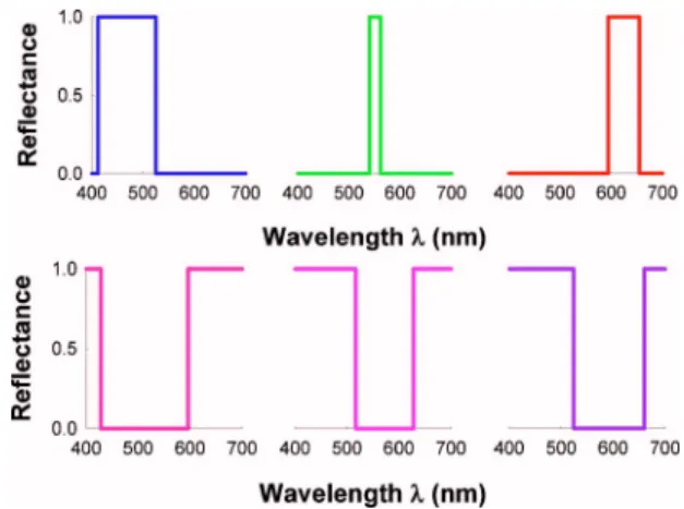
Two types of optimal colors are possible: type 1, with mountainlike spectral profiles, and type 2, with valleylike spectral profiles. Figure 1 shows several examples of both types of color stimuli, all of them with the same lumi-nance factor under the equienergetic illuminant encoded by the CIE-1931XYZstandard observer. The optimal col-ors do not really exist; that is, they are not found in na-ture and cannot be obtained by means of colorant formu-lation. Nevertheless, they serve to delimit the color solid of the human perception and to evaluate the colorimetric quality of colorants8–10: when colorants are near the Mac-Adam limits, a greater range of reproducible colors (color gamut) can be obtained. For instance, Pointer14,15used in 1980 these colorimetric data for comparing several indus-trial color gamuts.
The original MacAdam’s algorithm, based on the calcu-lation of the colorimetric purity, does not search system-atically all the optimal colors of the visible spectrum for a specific luminance factor. This means that the MacAdam limits plotted in the current literature are interpolated curves from a discrete and reduced set of original data. Moreover, the most usual illuminants in the literature8,9,16are always A, C, D65, and E, withYvalues above 10%.
We present in this work what we believe to be a new algorithm for systematically searching optimal colors for any illuminant (type F, P, D, etc.) and even for real lamps (discharge, fluorescents, LED, etc.), independently of the luminance factorY(lightnessL*) in the ]0, 100[ range. In
this way, the color solid should be completely graphed in several new color spaces, and we can determine how its shape and its content, associated with the variety of dis-tinguishable color sensations, with or without perceptual correspondence, depend on the illuminant–light source.
2. METHODS
Our algorithm is composed of two subalgorithms: one for calculating type 1 optimal colors and the other for
calcu-lating type 2 optimal colors. By default, the algorithm uses the following data:
(a) The visible spectrum range, for instance, from 380 to 780 nm.
(b) The spectral sampling, N, in this case is equal to 0.1 nm.
(c) The color-matching functions of the CIE-1931XYZ
standard observer17(with⌬= 1 nm), adequately interpo-lated to fit the spectral sampling (with⌬= 0.1 nm). Us-ing typical algebraic notation in colorimetry, the CIE color-matching functions are described by T
=关x¯ y¯ ¯z兴4001x3. Since these curves are smooth, linear interpolation is sufficient.18
(d) The spectral power distribution or spectrumS共兲of the illuminant, sampled at the same rate as the color-matching functions. In this way, the weighting tables for any illuminant and CIE-1931 observer combination are computed byT
⬘
=T· diag共S兲, where diag共S兲is the diagonal matrix of the illuminant vector S. In this case, we have used spline instead of linear interpolation, following the recommendations of the CIE,18 because the spectral curves for some illuminants and light sources curves are not so smooth.(e) The lightness valueL*with tolerance⌬L*. We use
these data instead of the luminance factorYbecause we want to analyze the color solid at constant lightness planes. The tolerance value⌬L*guarantees that optimal colors obtained for a certain lightness value are distrib-uted in a constant lightness plane, whose thickness (that is, the lightness difference between the lightest and the darkest optimal colors) does not surpass⌬L*. To work in
this way, the dependence ofL*onYfor all the range of the
luminance factor must be taken into account:
L*=
冦
903.3Y Yn , ifY/Yn艋0.008856 116冉
Y Yn冊
1/3 − 16, ifY/Yn⬎0.008856冧
, 共1兲withYn= 100 for the illuminant; if⌬L*=f共Y±⌬Y兲−f共Y兲 is
constant, then ⌬Y=
冦
100 903.3⌬L *, ifY共%兲艋0.8856 100冋
冉
⌬L * 116+冉
Y 100冊
1/3冊
3 − Y 100册
, ifY共%兲⬎0.8856冧
. 共2兲With these preliminaries, for each fixed lightness val-uesL*under any illuminant, our routine systematically finds the wavelengths 1 and 2, where the sudden
change of reflectance or transmittance happens (from 0 to 1, or opposite). That is, the spectra of the optimal colors in
Fig. 1 differ in the center and width but not height (al-ways 0 or 1).
This algorithm systematically searches the optimal col-ors along the selected spectral range. If the chosen spec-tral range is, for example, from 380 to 780 nm in steps of
Fig. 1. (Color online) Six examples of optimal colors (left: type 1; right: type 2) with luminance factorY= 20% under illuminant E and the CIE 1931XYZstandard observer. The transition wave-lengths1and2are, from left to right, as follows: 412.1–525.2, 540.0–562.0, 594.0–654.7, 428.0–596.0, 517.1–628.0, and 524.0– 660.1 nm.
0.1 nm, the algorithm has to look for all the possible pairs
1–2within 8,002,000 colorimetrically possible
combina-tions. Obviously, this algorithm, for each lightness value
L* and optimal color type, has a considerable
computa-tional cost. For example, with the algorithm implemented inMATLAB, the average computing time for each optimal color type and lightness is approximately 1 h with a Pen-tium IV computer. Obviously, this mainly depends on the wavelength step⌬: if, instead of taking⌬= 0.1 nm, we consider⌬= 1 nm, computing times are significantly re-duced. In this case, the subsequent reduction of the num-ber of optimal colors negatively affects the sampling qual-ity of the MacAdam limits.
Our algorithm consists of calculating the tristimulus valueYfrom an optimal wavelength pair, within the in-terval fixed by⌬L*. The condition imposed for our
algo-rithm for each optimal color type is described in the fol-lowing equations and is outlined in Fig. 2:
Type 1:Y= 100 y ¯ ·S
兺
k=i j y ¯共k兲·S共k兲苸关Y0−⌬Y,Y0+⌬Y兴, 共3兲 Type 2:Y= 100 y ¯ ·S冉
兺
k=1 i y ¯共k兲·S共k兲+兺
k=j N y ¯共k兲·S共k兲冊
苸关Y0−⌬Y,Y0+⌬Y兴, 共4兲where Y0 is the luminance factor calculated from the
lightness valueL*initially defined.
With each pair of limiting wavelengths,1共=i兲and2共=j兲,
and the illuminant–light source S共兲 it is very easy to generate the optimal color stimuli Coptimal共兲 as
optimal共兲*S共兲 withN spectral samples. Obviously, from
here one can almost immediately compute theXYZ tris-timulus values from the color-matching functions and en-code them into perceptual values in several color spaces (Fig. 3), such as CIELAB, SVF, DIN99d, and CIECAM02.
3. RESULTS
Since we initially calculated all the optimal colors of the color solid in the CIE-L*a*b*color space (Fig. 4), our
algo-rithm returns optimal colors within a lightness interval. To compute the color solid in other color spaces, we have to consider that the model’s equivalent variable to light-ness need not be constant for all of the lightlight-ness data set. This happens, for instance, with the CIECAM02 color space, where the lightnessJ depends on the achromatic response elicited by the stimulus. In any case, it should not be difficult to adapt the algorithm to the definition of lightness used in a particular model (Jin the CIECAM02 color space,Vin the SVF color space,L99din the DIN99d
color space, etc.)
Fig. 2. (Color online) Scheme of our algorithm in column for-mat. See text for more detail.
Fig. 3. General diagram for obtaining the color solid in several color spaces.
Fig. 4. Rösch–MacAdam color solid in the CIE-L*a*b* color
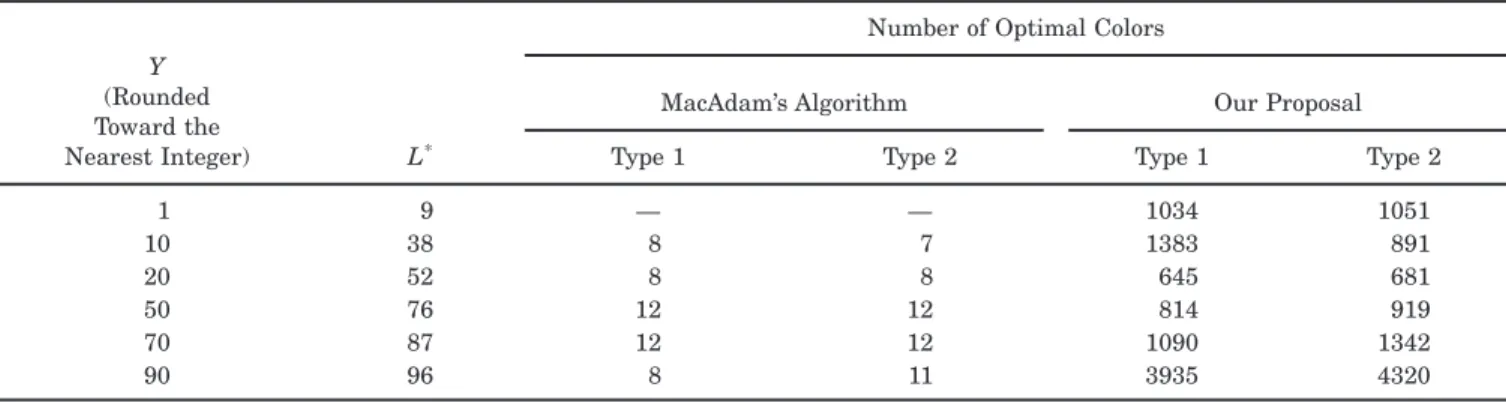
We have uniformly sampled the ]0, 100[ lightness inter-val, at one-by-one steps. As can be seen in Table 1, for in-stance, our algorithm and the one originally due to MacAdam,4 with the same wavelength step ⌬, yield a considerably different number of optimal colors for sev-eral luminance factors under illuminant C.
Another subject we bear in mind after the previous table is that the number of optimal colors obtained with our algorithm depends on the value ofL*(Fig. 5), as well
as on the tolerance⌬L*. If⌬L*is very small, for example, smaller than 0.005, the number of optimal colors will di-minish considerably, so the smoothness of the plotted MacAdam loci will be reduced. But if this parameter is great, for example, greater than 0.5, the number of opti-mal colors will be grouped in minicurves, the global rep-resentation of MacAdam loci will appear slightly stepped, and the graphic quality will decrease. Therefore, after testing several tolerance values we have found that⌬L*
= 0.01 is optimal. This lightness tolerance value will guar-antee that the MacAdam locus for each lightness plane is sufficiently smooth, rendering linear interpolation of these colorimetric data unnecessary.
A. Color Solid in Constant Lightness Planes
As we have just said, optimal color data associated with luminance factors lower than 10% and higher than 95% are not found in the literature. However, with our pro-posed method we can broaden the number of known opti-mal colors and find new ones for any luminance factor, from 0 to 100%. Taking into account Eq. (1), we can search any optimal color for lightness values in the [1, 100] interval, at one-by-one steps.
After looking at the previous table, it is clear that with our algorithm we will be able to delimit the MacAdam loci more accurately than with the original MacAdam algo-rithm, without graphical interpolation, as can be seen in Fig. 4. However, the sampling of the optimal color loci made with our algorithm in each color space is not uni-form, and it depends on the lightness value (Fig. 5). Inde-pendently of the color space or the illuminant/lamp se-lected, the MacAdam limits for high and low lightness values are better sampled than for intermediate lightness values, as can be seen in Fig. 5.
As the lightnessL*can be selected within the interval
]0, 100[, the complete figure of the color solid can be
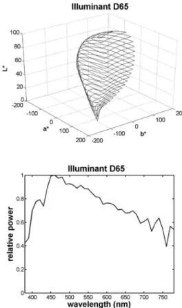
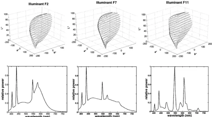
ob-tained for any illuminant or light source. Figure 6 shows the color solid in the CIEL*a*b*color space for three
fluo-rescent illuminants: F2, F7, and F11. As can be seen, the shape of the color solid depends on the illuminant. We clearly can see that the shape of the color solid obtained with illuminant F11 is quite different from the rest. We also show in Fig. 7 the color solid for three real lamps19: the standard high-pressure sodium lamp (HP1), the color-enhanced high-pressure sodium lamp (HP2), and the high-pressure metal halide lamp (HP3). As can be seen, the color solid for the HP1 lamp clearly differs from the rest. Therefore, perhaps it is possible to evaluate the color-rendering index of light sources from the number of distinguishable colors, estimated from the volume of its color solid. If this were possible, this colorimetric quality index for light sources would be absolute, without the ne-cessity of taking a reference illuminant, such as the cur-rent CIE color-rendering algorithm20–23 proposes. This idea has been applied in a preliminary way by us in par-allel with this work, and it will be summarized and dis-cussed in the next section.
We have also calculated the color solid for the color spaces (Fig. 8), such as CIECAM02, DIN99, and SVF, since these color spaces are more uniform than CIE-L*a*b*. We can see that these color solids are more
Table 1. Comparison between the Sampling of Optimal Colors, Using the Illuminant C and the CIE 1931 Standard Observer with the Same Spectral Sampling„⌬= 0.1 nm…, Obtained with MacAdam’s Algorithm4
and Our Algorithm
Y (Rounded Toward the
Nearest Integer) L*
Number of Optimal Colors
MacAdam’s Algorithm Our Proposal
Type 1 Type 2 Type 1 Type 2
1 9 — — 1034 1051 10 38 8 7 1383 891 20 52 8 8 645 681 50 76 12 12 814 919 70 87 12 12 1090 1342 90 96 8 11 3935 4320
Fig. 5. Effect of the luminance factorYover the (calculated op-timal color) symbol sampling of the MacAdam loci: the smaller MacAdam loci correspond toL*= 1 andL*= 98, while the larger
one corresponds toL*= 50. It was clearly seen that in the larger
locus the yellow–red quadrant is partially sampled, particularly for the red hues.
uniform, above all the color solids associated with the DIN99d and CIECAM02 color spaces because they look more spherical or homogeneous. The color solid in the SVF color space is not closed in the black vertex, unlike in the CIE-L*a*bcolor space (Fig. 4) and the rest (Fig. 8). In
the following section it will be discussed if the shape of the color solid ought really be more spherical or
homoge-neous in uniform color spaces, such as CIECAM02 and DIN99d, or if this result is purely coincidental.
B. Color Solid in Constant Hue-Angle Planes
As we advanced in the Introduction, in this work we also show a method to plot the color solid in constant hue
Fig. 6. Rösch–MacAdam color solid in the CIE-L*a*b*color space under three fluorescent illuminants: F2 (left), F7 (center), and F11
(right).
planes. The method basically consists of cutting up the color solid in vertical sections of constant hue. That is, we now try to draw the color solid共a*,b*,L*兲in constant hue
profiles withC*versusL*axes. To calculate thea*andb*
coordinates, it is necessary to obtain previously the chroma as a function of the angle huehab*, i.e.,hab* ver-susCab*, and we sometimes have to interpolate. In this case, although the curves are not very uniform, we have used the linear interpolation, since the spline interpola-tion does not show good results in the extreme values of the hue-angle interval. In future studies we will try to implement the Sprague interpolation algorithm proposed by the CIE.18So, we take 120 hue-angle values, between 0 and 360, at intervals of 3 deg, since a change of 3 deg en-sures that all the different Munsell hues14are considered, even in the SVF, DIN99d, and CIECAM02 color spaces. Therefore, we interpolate theC*value associated with the
hue angleh*; after that thea*andb*coordinates are
com-puted, and finally the color solid is plotted. This procedure is the same for all the color spaces, except that in the other spaces used we work with the colorfulness and not with the chroma. For instance, in the CIECAM02 color space,13 M is the adequate variable, the corresponding cardinal coordinates areaMandbM, and the hue angle is
defined in a conventional way from these cardinal coordi-nates.
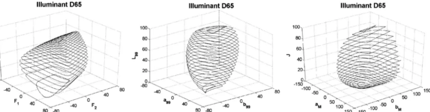
The color solids for the different color spaces for illumi-nants D65 and F11 and the real lamp HP1 are shown in Fig. 9, where we can also see the differences in the shape of the color solid, as we already saw in the color solid when it was plotted in constant lightness planes. If we represent graphically the complete color solid, the differ-ences due to the illuminant are very subtle (Fig. 9). So, a more compact visualization (Fig. 10) allows us to compare simultaneously different color solids under different illu-minants and light sources to analyze these differences better.
In Fig. 10, using different constant hue profiles in CIELAB associated with the primary Munsell hues, two continuous-spectrum illuminants, E and D65, are com-pared with a discontinuous-spectrum illuminant, F11, and a real light source, HP1, with a very peaked spec-trum, spanning correlated color temperatures from ap-proximately 2000 to 6500 K. Again, we can see greater differences among these illuminants in the following hue regions: purple (5P), blue–green (5BG), green (5G), and blue–purple (5PB).
However, these comparisons made in CIELAB are quite preliminary, and not completely effective, because we are not applying a common chromatic adaptation to the opti-mal color data in order to render the absolute colorimetric comparison, under the same reference illuminant. Among the uniform color spaces used in this work, with their cor-responding variables 共C,V兲 for SVF, 共C99,L99兲 for
DIN99d, and共M,J兲for CIECAM02, only the last one has an embedded chromatic adaptation transform, CAT02, which can be simultaneously applied to all previous data under the same internal or cortical illuminant. So, we have calculated the corresponding colors of the previous MacAdam loci under each illuminant–lamp by means of the CAT02 transform13(degree of adaptation orDfactor calculated by default,D= 0.9119) in order to make simul-taneously comparisons among them under the same illu-minant. The white point of this reference illuminant lies between the illuminants E and D65. Figure 11 shows these calculations in CIECAM02 with constant hue pro-files for the illuminants E, D65, and F11 and the real lamp HP1. Unlike Fig. 10, the greater similarities of color gamut among them are in the hue profiles 5P, 5B, and 5PB.
Making comparisons between pairs of illuminants in Fig. 11, and beginning with the E–D65 pair, it can be clearly seen in hue profiles 5GY, 5G, and 5BG that, for very pale and light colors, some distinguishable colors un-der illuminant E can exist without equivalent chromatic appearance under illuminant D65. That is, if we consider chromatic adaptation to our reference illuminant, the gamut for very light colors for the illuminant E in this hue region is higher than that of the illuminant D65. But, in hue region 5Y, the gamut of very light colors for the il-luminant D65 is higher that associated with the illumi-nant E. This superiority in color gamut of D65 over E in color gamut is more evident in the increase of bright, strong, and deep colors, never perceptible under illumi-nant E, in the hue regions 5RP, 5R, and 5YR. This inter-esting analysis of perceptible color gamuts under both il-luminants can be extended to more hue regions and with more graphic detail.
Proceeding analogously with the D65–F11 pair, again it can be clearly seen in Fig. 11 that we can perceive very light and bright greenish colors under illuminant F11 (along the range 5GY–5G–5BG) without perceptual corre-spondence under illuminant D65. In contrast, in the same hue regions, the perceptible color gamut under illuminant
Fig. 8. Rösch–MacAdam color solids for the CIE 1931 standard observer under the illuminant D65 in different perceptual color spaces: SVF (left), DIN99d (center), and CIECAM02 (right).
D65 is clearly higher than that of the illuminant F11 for strong and deep greenish colors. Similar analyses, and with more graphic detail, could be done in other hue re-gions (reds, oranges, etc.), but it is clear that the percep-tible color gamut of the illuminant D65 is greater than that of the illuminant F11. Nevertheless, from the previ-ous analysis it can also be inferred that, although the
number of discernible colors under illuminant D65, if it might be obtained exactly, would be higher than that as-sociated with the illuminant F11, not all perceptible col-ors under illuminant F11 do necessarily belong to the set of distinguishable colors of the illuminant D65 and vice versa.
Regarding the comparison HP1 versus D65, it is clear
Fig. 9. Rösch–MacAdam color solid under the illuminants D65 (left) and F11 (center) and the real lamp HP1 (right) in the color spaces CIE-L*a*b*, SVF, DIN99d, and CIECAM02. Sixty hue profiles have been taken to avoid aliasing.
that the color gamut under illuminant HP1, and with color correspondence under illuminant D65, is inside the color gamut of illuminant D65 for most hue regions, ex-cept for the hue region 5PB, specifically in the region of very dark and deep colors.
Finally, similar comparisons can be done with other illuminant–lamp pairs in Fig. 11, as, for example, E ver-sus F11 and HP1 verver-sus F11. But, definitively, it can clearly be seen that, when the same color correspondence over the color solids is applied under different illuminants–lamps, the greatest perceptible color gamuts are for the illuminants E and D65 and the lowest one is for the lamp HP1. In contrast, we have found that there can be perceptible colors under one illuminant–light
source without chromatic correspondence under other illuminants–light sources. In the next section, we discuss jointly all the results described up to this point, which could perhaps also be enlarged in future works.
4. DISCUSSION
In previous sections we have shown that the recalculation of optimal colors under several illuminants and light sources, encoded and three-dimensionally plotted as a color solid in several color spaces, has brought about some results and ideas that are worthwhile to recap and elabo-rate a bit more, even with additional results, because new
Fig. 10. (Color online) Constant hue-angle profiles of the Rösch–MacAdam color solid under several illuminants in the CIE-L*a*b*
共Cab*,L*兲diagram (illuminant F11: solid curve; HP1: dashed curve; E: dotted curve; and D65: dashed–dotted–dotted curve).
Fig. 11. (Color online) Constant hue-angle profiles of the Rösch–MacAdam color solid under several illuminants in the CIECAM02
interesting works about colorimetry of light sources and color perception can be separately derived from this work.
A. Concerning the Shape of the Color Solid in a Uniform Color Space
The three-dimensional plot of the color solid in several color spaces (Figs. 8 and 9), some of them quite uniform, gives rise to the question of whether the shape of a color solid in a perfectly uniform color space should be com-pletely spherical. Therefore, this subject is also linked with a comparative analysis of the uniformity of the color spaces used in this work. It was clear until now that the DIN99d and CIECAM02 spaces are the most uniform ones because they were designed with the aim of improv-ing the uniformity of older color spaces (CIELAB, SVF, etc). Due to this reason, as can be seen in Figs. 8 and 9, the color solids under any illuminant–lamp look more spherical or homogeneous in CIECAM02 and in DIN99d than in CIELAB or SVF. We might conclude that the CIECAM02 color space is a bit more uniform than the DIN99d color space. In fact, as this last one is based on the CIELAB color space, which has enough uniform de-fects in the purple region, particularly for very dark col-ors, a protuberance, but less emphasized, can still be seen in Figs. 8 (center) and 9 (right) for dark and deep purple colors. Therefore, we can conclude that the CIECAM02 color space, due to its uniformity, encodes the color solid with greater homogeneity. However, this does not mean necessarily that in a hypothetically perfectly uniform color space the color solid under illuminate D65, for in-stance, will be a perfect sphere. Taking Figs. 8, 9, and 11 into account, it is clear that the shape of the color solid under illuminant D65, or E, is rounded but not a perfect sphere. This is caused by the spectral tuning of the illuminant–lamp spectrum with the color-matching func-tions, above all with ¯y共兲 and the luminous efficiency curveV共兲, that is, by the shape and area of the product
S共兲·V共兲. Indeed, as the original MacAdam’s works4,5 proved and as can be seen in classical colorimetry text-books, the greater variety of light colors appear in the green–yellow (GY) hue region. Due to this reason, taking into account the approach of the constant lightness pro-files, the snap of the MacAdam loci toward the absolute white is not homogeneous or circular. As is easily seen in Figs. 4–8, there is always a protuberance on the upper level of all the color solids, independently of the illuminants/lamps and/or color spaces used, but displaced from green to orange depending on the correlated color temperature (chromaticity) of the illuminant–lamp. Consequently, it is not a necessary condition that the color solid encoded by the most uniform color space should be plotted as a perfect sphere. For this reason, the Munsell color tree is clearly asymmetric, with longer branches present at high Munsell values for (typically) yellowish hues and at low Munsell values for (typically) purple hues. In the case of the CIECAM02 color space, the snap of the color solid toward the absolute black will be always more homogeneous or circular than that toward the absolute white. Therefore, the MacAdam limits with very high lightness never will be homogeneous or circular, except in a quasi-triangle region around the yellowness perceptual axes. One further work to be
devel-oped from this issue would be to use, as a reference, the color solid corresponding to the perceptually determined data of the Munsell Renotation System (or a similar data set, for instance, Natural Color System data) with ex-trapolated specification for the optimal colors24,25 and to determine how much the color solids in question depart from this.
On the other hand, applying CIECAM02, we have found that the shape of the color solid can change significantly according to the degree of chromatic adapta-tion or factor D. In the above figures associated with CIECAM02, this color model has been always applied by calculating by default the corresponding factor
D共=0.919兲. But, testing other D values, for instance,
D= 0 (without adaptation) and D= 1 (complete adapta-tion), the shapes of the color solid for the same illuminant–lamp can be very different. In Fig. 12 the color solids at constant lightness planes for three illuminants– lamps (HP1, F11, and D65) are shown, visualized from top to bottom, for two degrees of adaptation (D= 0 and
D= 1). As we can see, the color solids varying less are those associated with the illuminant D65, while those varying more belong to the lamp HP1. Color solids asso-ciated with the illuminant E with this new test have not been plotted because their changes were minimal with both adaptation conditions, so this reinforces the fact that the cortical or internal illuminant for the CIECAM02 color model is nearer in chromaticity to the illuminant E than to the illuminant D65. Taking the last figure into ac-count, since human color perception always works with chromatic adaptation, in a lesser or greater degree, but never withD= 0, the right side of Fig. 12 represents an alternative way of viewing in a perceptual color space, without chromatic adaptation, the MacAdam limits shown for many years in chromaticity diagrams8–10 as CIE-xy, CIE-u
⬘
v⬘
, etc. As can be clearly seen in this fig-ure, the HP1 data indicate a strong colorimetric shift to-ward the orange region of solid color (the equal-energy white stimulus would be perceived as orange) due to the chromaticity (color temperature) of the light source, above all for very light colors. This accentuated colorimetric shift is partially neutralized by chromatic adaptation, which serves to justify the perceptual phenomenon of color constancy.However, regarding the cases with complete chromatic adaptation, which are the ones most similar to the factor
Dcalculated by default in the previous section, it can also be seen in Fig. 12 and likewise in Fig. 11, if only the en-velope of the constant lightness planes of color solids is taken into account, that there are perceptible colors un-der illuminant F11 in the green–yellow quadrant, with middle lightness, which are not perceptible under illumi-nant D65, not even under lamp HP1. Furthermore, from the top view, it seems that the region covered by the D65 color solid is altogether greater than that of the illumi-nant F11. So, this result again proves that there can be perceptible colors under one illuminant/light source with-out perceptual correspondence under another illuminant– light source, even if the first illuminant had in all a more limited number of discernible colors than the second illu-minant.
non-uniformity of the color solid toward the black when it is encoded by SVF color space. Despite the fact that this color space was designed with the aim of plotting uni-formly the constant lightness Munsell loci, the mathemat-ics of this color model causes the corresponding color solid not to taper homogeneously toward the absolute black, unlike what happens toward the absolute white (Figs. 8 and 9). Since this color model is fitted to the Munsell At-las, its equations include a threshold value共S0= 0.43兲 in
order to adapt the scaling of the Munsell value. So, forY
values lower than 0.43% 共L*⬍3.88兲, all optimal colors
with lower lightness are encoded with valueVSVF= 0. This
colorimetric behavior is common in any physiological color space, with a threshold value below which the re-sponse is zero, not negative. Due to this, the color solid plotted in this color space does not taper toward a point (absolute black), since there is a gap between the last graphed MacAdam locus and the absolute black. Thus, the cutoff in the lowermost part of the color solid in the
SVF color space is in agreement with the physiological premises imposed. In spite of this, it seems adequate to improve the modeling of the SVF color space for very dark colors.
B. Concerning the Content of the Color Solid according to Different Light Sources
The changes in the shape of the color solid with the spec-tral content of the illuminant–light source raise the issue of the differences in colorimetric quality among illumi-nants and light sources. This topic will be analyzed in more detail in Subsection 4.C, but it is also connected with the questions of how many color sensations, with a given illuminant–light source, we can distinguish and why this depends on its spectrum and its chromaticity. To understand this matter better, it is necessary to make si-multaneous comparisons of color solids under several illuminants–lamps but taking chromatic adaptation into
Fig. 12. Top view of some color solids under several illuminants–lamps in the CIECAM02 color space with different chromatic adap-tation degrees (left:D= 1; right:D= 0). (The MacAdam locus with the solid curve corresponds to the highest constant lightness plane.)
account, for instance, using the CAT02 transform of the CIECAM02 color appearance model. For this reason, Fig. 11, obtained with CIECAM02, is a correct representation of the color solid (with constant hue profiles) under the same perceptual correspondence, that is, under the refer-ence or internal (cortical) illuminant of the human visual system, similar in chromaticity to the equienergetic illu-minant. From this figure, and all cited above, we may con-clude the following:
• The color solids associated with illuminants–lamps, with correlated color temperatureTClower than 5500 K,
will have color gamuts smaller than those associated with illuminants–lamps withTCequal or higher than 5500 K.
This is clearly proved for the lamp HP1, often used in ur-ban lighting, and the fluorescent illuminant F11, often used in interior lighting. It is a pending matter whether in a higher range of color temperature there is an upper limit above which the color gamut will diminish. To test this, we have also calculated the color solid corresponding
to the illuminant D100, with TC= 10,000 K, and it has
been plotted in the DIN99d color space by applying previ-ously on the optimalXYZ data the CAT02 transform for the illuminant D65, as was done for the lamp HP1 and the illuminants A, F11, E, and D65, with the aim of cov-ering roughly a large chromaticity range. We now have used the DIN99d color space because it is more coherent to show corresponding colors in a color space different from that associated with a one-color appearance model (CIECAM02), which describes and applies a chromatic adaptation transform (CAT02). A top view (Fig. 13) of the MacAdam loci associated with these illuminants–lamps supports what we said above: forTC⬍5500 K, the lower
the correlated color temperature, the smaller the distin-guishable color gamut. But, in contrast, we have not found a similar behavior forTChigher than 10,000 K,
al-though is it possible that from any point of the关10,000, +⬁兴K range the reduction of the gamut volume again turns up. However, this preliminary corollary cannot be
Fig. 13. Top view of several color solids under several illuminants/lamps, with the same color correspondence to illuminant D65, in the DIN99d color space. From top to bottom and from left to right: lamp HP1共TC= 1960 K兲, illuminant A共TC= 2856 K兲, illuminant F11
共TC= 4000 K兲, illuminant E共TC= 5500 K兲, illuminant D65共TC= 6500 K兲, and illuminant D100共TC= 10,000 K兲. (The MacAdam locus with
correct for all very narrowband lamps, for instance, two-band lamps, real or simulated. Hence, further research should be done on this issue.
• Taking into account the analyses derived from Figs. 11, 13, and 14, we have found that there are color sensations under one illuminant–lamp, near the MacAdam limits, which do not have perceptual correspondence under other illuminants–lamps. But, moreover, we have proved that there can be illuminants–lamps with reduced color gam-uts in comparison with other illuminant–gamut pairs, which have a small but significant number of color sensa-tions imperceptible under those illuminants/lamps with greater color gamuts. Therefore, these conclusions imply that the number of colors discernible by the human visual system can be unlimited26because it needs not be associ-ated with only one illuminant–lamp, but, regarding the variety of natural or artificial light sources, we can pre-dict and verify new color sensations that do not corre-spond with known illuminants/lamps. Some examples about this involving some hue regions have been given in Fig. 11 and can be again given in Figs. 13 and 14, above all with the aim of comparing the illuminants A and D100 relative to the illuminant D65. Nevertheless, perhaps this preliminary analysis and its conclusions might be en-larged with more graphic detail, and with greater statis-tical diversity of illuminants and lamps, in a future work because this would be very interesting for the lighting community, for its applications (museums, sport, and arts entertainments, etc.), and for the CIE.
• Regarding the quantity and variety of colors distin-guishable by the human visual system and taking the re-sults shown in Fig. 12 into account, where the shape and volume of the color solids are compared as a function of the degree of chromatic adaptation, it is clear that if our visual system did not use chromatic adaptation the num-ber of discernible colors would be much greater, with mi-nor perceptual correspondence among illuminants and light sources. Therefore, the color constancy phenomenon,27–31based at the first stages on a chromatic
adaptation transform, means from a evolutionary point of view an adaptive mechanism to reduce the variability of perceptually noncorresponding distinguishable colors. Thanks to this adaptive mechanism, the result of the evo-lution of several million years, our primate predecessors achieved a quasi-invariant system for encoding color in front of chromaticity changes of ambient light, clearly ad-vantageous for establishing quasi-constant recognition patterns of objects and scenes very important for survival.
C. Concerning the Proposal of an Absolute Colorimetric Index of Illuminants and Light Sources Based on the Volume of the Color Gamut
As we said above, it is clear that the shape and volume of the color solid depends on the spectral content of the illuminant–light source. Therefore, we may say that the greater the gamut volume, the greater the number of dis-tinguishable colors. Then we could propose a colorimetric quality index based on this condition for classifying any illuminant/lamp. This colorimetric quality index among light sources would be absolute, with no need for using a reference illuminant, such as the current CIE color-rendering algorithm proposes. Therefore, what we need is to find one or several methods for calculating the gamut volume involving directly, for instance, the estimation of the total number of distinguishable colors inside the color solid. In a preliminary work,32done by ourselves, several methods for calculating the number of distinguishable colors inside the color solid were tested (Table 2). The first method consists of computing the partial counts of distin-guishable colors for each constant lightness MacAdam lo-cus encoded by CIECAM02, with a lightness step⌬L*= 1,
from 1 to 100, by a squares-packing method with unity area, without overlap, inside each MacAdam locus. In this way, the sum of these partial counts from L*= 1 to L*
= 100 gives the total number of distinguishable colors un-der each illuminant/light source. An alternative method, which gives similar results, consists of using the convex Fig. 14. (Color online) Constant hue-angle profiles of the Rösch–MacAdam color solid under several illuminants, with the same color correspondence to illuminant D65, in the DIN99d共C99,L99兲diagram (illuminant F11: solid curve; HP1: short-dashed curve; D65: dotted
hullfunction by MATLABfor constant lightness MacAdam
loci. The third method is named the ellipses-packing method. This takes Krauskopf and Gegenfurtner’s dis-crimination model,33 based on psychophysical data into account and works by filling the constant lightness Mac-Adam loci, previously transformed by the CAT02 trans-form under illuminant E, with discrimination ellipses in-creasing in area with inin-creasing distance from the achromatic point in a modified MacLeod–Boynton chro-maticity diagram. Consequently, again accumulating the partial counts of nonoverlapped ellipses or distinguish-able colors for each constant lightness MacAdam locus fromL*1 toL*100, with lightness step⌬L*= 1, we can es-timate the total number of distinguishable colors inside the color solid for any light source.
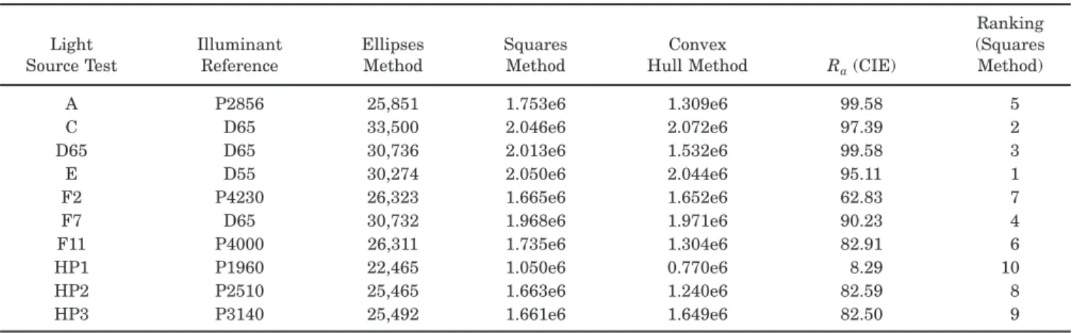
In Table 2 we show the preliminary results applying these three packing methods for several illuminants (A, C, D65, E, F2, F7, F11) and lamps (HP1–HP3), and they are compared with the standard CIE color-rendering algorithm.20,21 The three packing methods give absolute results of colorimetric quality, since they do not depend on a reference illuminant, as the current CIE algorithm does. However, despite the fact that there is a very good correlation in the ordering scale of quality in the three methods relative to the CIE algorithm, the magnitude of the numerical results in the three methods is very differ-ent. Thus, we might say that in applying the squares-packing (convex hull) method the number of distinguish-able colors under each illuminant/lamp is estimated by excess. In contrast, in applying the ellipses-packing method, the number of distinguishable colors is estimated by defect. Therefore, we think that much more work is needed, for instance, testing a spheres-packing method in the most uniform color space available, in order to make a careful study of this subject concerning the colorimetry of light sources and color perception.
However, these methods and their preliminary results could be useful to develop new applications in color imaging, as, for instance, comparing the color gamuts of color devices,34–36 and in lighting design (museums, sports, TV, cinema, etc.). This could even be applied in or-der to evaluate the distinguishable colors of animal
vision, such as dichromatic, trichromatic, or higher-dimensionality vision, provided that the internal model of chromatic discrimination and encoding was known for each species.
On the other hand, it could be highly questionable if the gamut volume alone is suitable as a quality index in this sense. When not also taking the shape of the color solid into account, the gamut volume may say little about color-rendering capabilities. Thus, the great challenge should be to find a parameter that depends on both vol-ume and shape. For instance, and to illustrate this, one can imagine two (theoretical) color gamuts, one repre-sented by a spherical color solid centered at the midpoint of the achromatic axes and the other by a hemisphere of the same volume and with the achromatic axes coinciding with a diameter of its base. There is no question that the former should give the highest colorimetric quality index. Taking into account this and the preliminary results shown in this subsection (Table 2), it seems that the cal-culation of an absolute colorimetric quality index from knowledge of the color gamut volume and shape is far from trivial. In spite of this, one possible solution could be a calculation of an intersection volume of two color gam-uts, A and B(this one as reference, for instance, as the illuminant E has been used in Table 2), as the average of
A\ (the intersection ofAandB) andB\ (the intersection ofAandB). In contrast, this fact would mean a return to the relative colorimetric index of illuminants and light sources. But, at least, all illuminants and real lamps would be normalized by the same reference illuminant, so it could be considered as a common (absolute) colorimetric index.
5. CONCLUSIONS
In this work we have improved the algorithm for calculat-ing the optimal colors proposed originally by MacAdam. The algorithm can be applied at any lightness value, so the color solid can be well sampled either in constant lightness planes or in constant hue planes for any color space. Unlike the irregularly shaped color solid obtained in CIELAB, the color solids associated with the most
cur-Table 2. Total Number of the Distinguishable Colors under Several Illuminants and Light Sources according to Several Packing Methods of Constant Lightness MacAdam Loci
Light Source Test Illuminant Reference Ellipses Method Squares Method Convex
Hull Method Ra(CIE)
Ranking (Squares Method) A P2856 25,851 1.753e6 1.309e6 99.58 5 C D65 33,500 2.046e6 2.072e6 97.39 2 D65 D65 30,736 2.013e6 1.532e6 99.58 3 E D55 30,274 2.050e6 2.044e6 95.11 1 F2 P4230 26,323 1.665e6 1.652e6 62.83 7 F7 D65 30,732 1.968e6 1.971e6 90.23 4 F11 P4000 26,311 1.735e6 1.304e6 82.91 6 HP1 P1960 22,465 1.050e6 0.770e6 8.29 10 HP2 P2510 25,465 1.663e6 1.240e6 82.59 8 HP3 P3140 25,492 1.661e6 1.649e6 82.50 9
rent perceptual color spaces, DIN99d and CIECAM02, look more spherical or homogeneous. However, this result does not imply that the color solid should be perfectly spherical in an ideal uniform color space, as we discussed above. Despite this, we think it would be interesting to determine in the future whether some characteristic of the color solid could serve as a test of the uniformity of a color appearance model. In the case of the SVF model, a uniformity defect around very dark colors was found due to the mathematics of that color model.
Once the color solids for different illuminants and light sources are shown, it can be seen that their shape and content clearly depend on the associated illuminant. Therefore, we can also conclude that the number of dis-tinguishable colors, evaluated as the gamut volume, could depend on the associated illuminant. Furthermore, some interesting corollaries have been derived from both main conclusions about the colorimetry of light sources and color perception, which would be interesting to extend more profoundly in the future:
• The color gamuts associated with illuminants/lamps, whose correlated color temperature TC was inside the
关5500, 10,000兴K interval, are greater than those associ-ated with illuminants/lamps with their TC outside the
cited interval. If TC moves enough from 5500 K, the
gamut volume will diminish in a uniform color space. However, this preliminary corollary cannot be correct for very narrowband lamps, for instance, two-band lamps, real or simulated. Hence, further research should be done to elucidate this open question.
• Applying the same color correspondence among optimal color data for each illuminant/lamp, we have found that there are distinguishable colors under one illuminant/lamp without perceptual correspondence un-der other illuminants/lamps, even though its gamut vol-ume was small. This means that the number of colors dis-cernible by the human visual system is unlimited because it cannot be associated with a single illuminant/lamp, but, in accordance with the variety of natural and artificial light sources, we can predict and verify new color sensa-tions that do not match those of other known illuminants/ lamps.
• An additional conclusion from above is that color con-stancy, based at the first stages on a chromatic adaptation transform, can be also understood as an adaptive mecha-nism reducing the diversity of distinguishable colors without common perceptual correspondence with mul-tiple illuminants/lamps.
• Finally, it has been proved with these preliminary re-sults that it is possible to define an absolute colorimetric quality index for any illuminant/light source, based on the computation of the number of distinguishable colors in-side the color solid. This proposal could be used as an al-ternative method to the (relative) color-rendering algorithm20 proposed by CIE. The proposed methods in these calculations could also be used to evaluate and com-pare color gamuts of color-imaging devices34–36and even of other natural vision systems (dichromacy, trichromacy, etc.). However, it seems adequate to work more much in the future with a colorimetric parameter for classifying il-luminants and real lamps, taking into account both the
volume (number of distinguishable colors) and the shape of the associated color solid.
Consequently, although the original aim of this work was the improvement of the method for calculating and plotting optimal colors, originally developed by Mac-Adam, the analysis of the shown findings have given rise to very interesting preliminary conclusions about the colorimetry of light sources and color perception, which are worthwhile to study in the coming years. The poten-tial applications of this work, and those derived from it, could be numerous for lighting design, color imaging, color perception in animal vision, etc.
ACKNOWLEDGMENTS
This research was supported by the Ministerio de Edu-cación y Ciencia, Spain, under grant DPI2005-08999-C02-02, and by the Conselleria d’Empresa, Universitat i Cièn-cia of the Generalitat ValenCièn-ciana, Spain, under grant IIARC0/2004/59. The authors thank the reviewers for their advice, helpful comments, and suggestions, particu-larly for the comments incorporated in our discussion.
Corresponding author F. Martínez-Verdú can be reached by e-mail at [email protected].
REFERENCES
1. R. G. Kuehni,Color Space and Its Divisions: Color Order from Antiquity to the Present(Wiley, 2003).
2. G. Wyszecki and W. S. Stiles,Color Science: Concepts and Methods, Quantitative Data and Formulae, 2nd ed. (Wiley, 1982), pp. 179–184.
3. R. S. Berns,Billmeyer and Saltzman’s Principles of Color Technology, 3rd ed. (Wiley, 2000).
4. D. L. MacAdam, “Maximum visual efficiency of colored materials,” J. Opt. Soc. Am.25, 316–367 (1935).
5. D. L. MacAdam, “Theory of the maximum visual efficiency of colored materials,” J. Opt. Soc. Am.25, 249–252 (1935). 6. E. Schrödinger, “Theorie der Pigmente von grösster
Leuchtkraft,” Ann. Phys.62, 603–622 (1920).
7. S. Rösch, “Fortschritte der Mineral,” Kristallogr. Petrogr. 13, 143 (1929).
8. R. G. Kuehni,Color Space and Its Divisions: Color Order from Antiquity to the Present(Wiley, 2003), pp. 91, 359. 9. R. S. Berns,Billmeyer and Saltzman’s Principles of Color
Technology, 3rd ed. (Wiley, 2000), pp. 62, 143.
10. R. W. G. Hunt,The Reproduction of Colour, 6th ed. (Wiley, 2004), pp. 88–90.
11. T. Seim and A. Valberg, “Towards a uniform color space: a better formula to describe the Munsell and OSA color scales,” Color Res. Appl.11, 11–24 (1986).
12. G. Cui, M. R. Luo, B. Rigg, G. Roesler, and K. Witt, “Uniform colour spaces based on the DIN99 colour-difference formula,” Color Res. Appl.27, 282–290 (2002). 13. CIE, A Colour Appearance Model for Colour Management
Systems: CIECAM02, CIE 159:2004 (Commission Internationale de l’Eclairage, 2004).
14. M. R. Pointer, “The gamut of real surface colours,” Color Res. Appl.5, 145–155 (1980).
15. M. R. Pointer, “Request for real surface colours,” Color Res. Appl.27, 374 (2002).
16. N. Ohta and A. Robertson,Colorimetry: Fundamentals and Applications(Wiley, 2005), pp. 215.
17. G. Wyszecki and W. S. Stiles,Color Science: Concepts and Methods, Quantitative Data and Formulae, 2nd ed. (Wiley, 1982), pp. 725–735.
for Use in Colour Computations, CIE 167:2005 (Commission Internationale de l’Eclairage, 2005).
19. CIE, Colorimetry, 3rd ed., CIE 15:2004 (Commission Internationale de l’Eclairage, 2004).
20. CIE, Method of Measuring and Specifying Colour Rendering Properties of Light Sources, CIE 13.3:1995 (Commission Internationale de l’Eclairage, 1995).
21. CIE, CIE Collection 1999, Vision and Colour, Physical Measurement of Light and Radiation, Research Note: Colour Rendering, TC 1-33 Closing Remarks, CIE 135/ 2:1999 (Commission Internationale de l’Eclairage, 1999). 22. C. van Trigt, “Color rendering, a reassessment,” Color Res.
Appl.24, 197–206 (1999).
23. J. A. Worthey, “Color rendering: asking the question,” Color Res. Appl.28, 403–412 (2003).
24. D. B. Judd and G. Wyszecki, Color in Business, Science, and Industry, 3rd ed. (Wiley, 1975), pp. 267.
25. R. W. G. Hunt,The Reproduction of Colour, 6th ed. (Wiley, 2004), pp. 162–163.
26. R. G. Kuehni,Color Space and Its Divisions: Color Order from Antiquity to the Present(Wiley, 2003), pp. 202. 27. S. D. Hordley and G. D. Finlayson, “Reevaluation of color
constancy algorithm performance,” J. Opt. Soc. Am. A23, 1008–1020 (2006).
28. A. Lewis and L. Zhaoping, “Are cone sensitivities determined by natural color statistics?” J. Vision 6, 285–302 (2006).
29. Y. Nayatani, “Development of chromatic adaptation
transforms and concept for their classification,” Color Res. Appl.31, 205–217 (2006).
30. S. D. Hordley, “Scene illuminant estimation: past, present, and future,” Color Res. Appl.31, 303–314 (2006).
31. D. H. Brainard, P. Longère, P. B. Delahunt, W. T. Freeman, J. M. Kraft, and V. Xiao, “Bayesian model of human color constancy,” J. Vision6, 1267–1281 (2006).
32. E. Perales, F. Martínez-Verdú, V. Viqueira, M. J. Luque, and P. Capilla, “Computing the number of distinguishable colors under several illuminants and light sources,” in Proceedings of Third IS&T European Conference on Colour Graphics, Imaging and Vision(Society for Imaging Science and Technology, 2006), pp. 414–419.
33. J. Krauskopf, “Higher order color mechanisms,” inColor Vision: From Genes to Perception, K. R. Gegenfurtner and L. T. Sharpe, eds. (Cambridge U. Press, 1999), pp. 310. 34. U. Steingrímsson, K. Simon, W. Steiger, and K. Schläpfer,
“The gamut obtainable with surface colors,” inProceedings of First IS&T European Conference on Colour Graphics, Imaging and Vision (Society for Imaging Science and Technology, 2002), pp. 287–291.
35. CIE,Criteria for the Evaluation of Extended-Gamut Colour Encodings, CIE 168:2005 (Commission Internationale de l’Eclairage, 2005).
36. F. Martínez-Verdú, M. J. Luque, P. Capilla, and J. Pujol, “Concerning the calculation of the color gamut in a digital camera,” Color Res. Appl.31, 399–410 (2006).