Spam email filtering using network-level properties

Spam Email Filtering

Using Network-Level Properties

Paulo Cortez1, Andr´e Correia1, Pedro Sousa3, Miguel Rocha3, and Miguel Rio2 1

Dep. of Information Systems/Algoritmi, University of Minho, 4800-058 Guimar˜aes, Portugal,

[email protected]

WWW home page:http://www3.dsi.uminho.pt/pcortez

2

Dep. of Informatics, University of Minho, 4710-059 Braga, Portugal,

{pns, mrocha}@di.uminho.pt

3 _{Department of Electronic and Electrical Engineering, University College London,}

Torrington Place, WC1E 7JE, London, UK,

[email protected]

Abstract. Spam is serious problem that affects email users (e.g. phish-ing attacks, viruses and time spent readphish-ing unwanted messages). We propose a novel spam email filtering approach based on network-level attributes (e.g. the IP sender geographic coordinates) that are more persistent in time when compared to message content. This approach was tested using two classifiers, Naive Bayes (NB) and Support Vec-tor Machines (SVM), and compared against bag-of-words models and eight blacklists. Several experiments were held with recent collected le-gitimate (ham) and non lele-gitimate (spam) messages, in order to simulate distinct user profiles from two countries (USA and Portugal). Overall, the network-level based SVM model achieved the best discriminatory performance. Moreover, preliminary results suggests that such method is more robust to phishing attacks.

Keywords: Anti-Spam filtering, Text Mining, Naive Bayes, Support Vector Machines

1

Introduction

Email is a commonly used service for communication and information sharing. However, unsolicited e-mail (spam) emerged very quickly after email itself and currently accounts for 89% to 92% of all email messages sent [11]. The cost of sending these emails is very close to zero, since criminal organizations have access to millions of infected computers (known as botnets) [15]. Spam consumes resources, such as time spent reading unwanted messages, bandwidth, CPU and disk [6]. Also, spam is an intrusion of privacy and used to spread malicious content (e.g. phishing attacks, online fraud or viruses).

The majority of the current anti-spam solutions are based on [3]: Content-Based Filtering (CBF) and Collaborative Filtering (CF). CBF is the most popu-lar anti-spam approach, using message features (e.g. word frequencies) and Data

Mining (DM) algorithms (e.g. Naive Bayes) to discriminate between legitimate (ham) and spam messages. CF works by sharing information about spam mes-sages. One common CF variant is the DNS-based Blackhole List (DNSBL), also known as blacklist, which contains known IP addresses used by spammers. CF and CBF can also be combined. For example, a blacklist is often used at a server level to tag a large number of spam. The remaining spam can be detected later by using a personalized CBF at the client level (e.g. Thunderbird SpamBayes, http://www.entrian.com/sbwiki).

Spam content is very easy to forge in order to confuse CBF filters. For ex-ample, normal words can be mixed into spam messages and this heavily reduces the CBF performance [13]. In contrast, spammers have far less flexibility in changing network-level features. Yet, the majority of the spam research gives attention to content and the number of studies that address network-level prop-erties is scarce. In 2005, Leiba et al. [9] proposed a reputation learning algorithm that is based on the network path (from sender to receiver) of the message. Such algorithm obtained a high accuracy when combined with a CBF bayesian filter. Ramachandran and Feamster [15] have shown that there are spam/ham differ-ences for several network-level characteristics (e.g. IP address space), although the authors did not test these characteristics to filter spam using DM algorithms. More recently, transport-level properties (e.g. TCP packet stream) were used to classify spam messages, attaining a classification accuracy higher than 90% [1]. In this paper, we explore network-level characteristics to discriminate spam (see Section 2.1). We use some of the features suggested in [15] (e.g. operating system of sender) and we also propose new properties, such as the IP geographic coordinates of the sender, which have the advantage of aggregating several IPs. Moreover, in contrast with previous studies (e.g. [9, 1]), we collected emails from two countries (U.S. and Portugal) and tested two classifiers: Naive Bayes and Support Vector Machines (Section 2.2). Furthermore, our approach is compared with eight DNSBLs and CBF models (i.e. bag-of-words) and we show that our strategy is more robust to phishing attacks (Section 3).

2

Materials and Methods

2.1 Spam Telescope Data

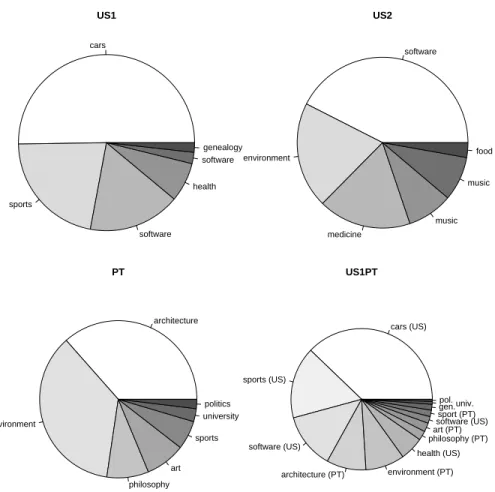
To collect the data, we designed and developed the spam telescope repository. The aim of this repository is to perform a longitudinal and controlled study by gathering a significant slice of the world spam traffic. Spam was harvested by setting several spam traps; i.e. fake emails that were advertised through the Internet (e.g. Web pages). To collect ham, we created email addresses what were inscribed in moderated mailing lists with distinct topics. Figure 1 shows the proportions of mailing list topics that were used in our datasets. For both spam and ham collection, we tried to mimic real users from two countries: U.S. and Portugal (PT). For instance, we first registered a U.S. domain (.com) and then set the corresponding Domain Name System (DNS) Mail Exchange (MX) record. Next, the USA spam traps were advertised in USA popular Web sites and the

USA ham emails were inscribed in 12 USA mailing lists. A similar procedure was taken to harvest the Portuguese messages (e.g. .pt domain).

cars sports software health software genealogy US1 software environment medicine music music food US2 architecture environment philosophy art sports university politics PT cars (US) sports (US) software (US) architecture (PT) environment (PT) health (US) philosophy (PT)

art (PT)software (US)

sport (PT)gen.

univ. pol.

US1PT

Fig. 1.Pie charts showing the distribution of mailing list topics for each dataset

All spam telescope messages were gathered at a specially crafted server. This server uses virtual hosting to redirect addresses from distinct Internet domains and runs a customized Simple Mail Transfer Protocol (SMTP) program called Mail Avenger (http://www.mailavenger.org). We set Mail Avenger to tag each received message with the following information:

– IP address of the sender and a traceroute to this IP;

– Operating System (OS) of the sender, as estimated from a passive p0f TCP fingerprint;

– lookup at eight DNSBLs: cbl.abuseat.org (B1), dnsbl.sorbs.net (B2), bl.-spamcop.net (B3), sbl-xbl.spamhaus.org (B4), dul.dnsbl.sorbs.net (B5), zen.-spamhaus.org (B6), psbl.surriel.com (B7) and blackholes.five-ten-sg.com (B8).

The four network-level properties used in this study are presented in Table 1. Instead of using direct IP addresses, we opt for geographic coordinates (i.e. latitude and longitude), as collected by querying the free http://ipinfodb.com database. The geographic features have the advantage of aggregating several IPs. Also, it it known that a large fraction of spam comes from specific regions (e.g. Asia) [15]. The NHOP is a distance measure that was computed using the traceroute command. The passive OS signatures were encoded into four classes: windows – if from the MS family (e.g. windows 2000); linux (if a linux kernel is used); other (e.g. Mac, freebsd, openbsd, solaris); and unknown (if not detected).

Table 1.Network-level attributes

Attribute Domain

NHOP – number of hops/routers to sender{8,9,. . .,65}

Lat. – latitude of the IP of sender [-42.92◦,68.97◦] Long. – longitude of the IP of sender [-168.10◦,178.40◦]

OS – operating system of sender {windows,linux,other,unknown}

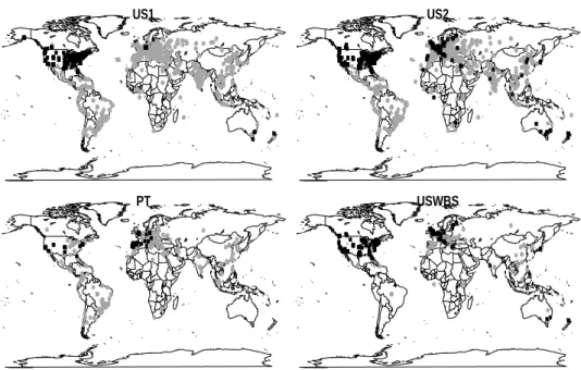
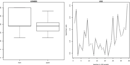
In this study, we collected recent data, from April 21st April to November 9th 2009. Five datasets were created in order to mimic distinct and realistic user profiles (Table 2). The US1 set uses ham from 6 mailing lists whose members are mostly U.S. based, while US2 contains ham from different U.S. lists and that is more spread through the five continents (Figure 2). Regarding the spam, the data collected from the U.S. traps was added into US1 and US2, while PT includes only features extracted from Portuguese traps. The mixture of ham and spam was based on the time that each message was received (date field), which we believe is more realistic than the sampling procedure adopted in [12]. Given the large number of experiments addressed in this work, for US1, US2 and PT we opted to fix the global spam/ham ratio at 1. Yet, it should be noted that the spam/ham ratios fluctuate through time (right of Figure 4). The fourth set (US1PT) merges the data from US1 and PT, with the intention of representing a bilingual user (e.g. Portuguese but working in U.S.). Finally, the U.S. Without Blacklist Spam (USWBS) contains ham and spam from US2. The aim is to mimic a hybrid blacklist-filter scenario, thus all spam that was detected by any of the eight DNSBLs was removed from US2. For this last set, we set the spam/ham ratio to a realistic 0.2 value, since in such scenario most spam should be previously detected by the DNSBLs. Figures 2, 3 and 4 show several examples of ham/spam differences when analyzing the network-level attributes.

Table 2.Summary of the Spam Telescope corpora

setup ham main #mailing #ham total spam time

language lists senders size /ham period

US1 English 6 343 3184 1.0 [23/Apr./09,9/Nov./09]

US2 English 6 506 3364 1.0 [21/Apr./09,9/Nov./09]

PT Portuguese 7 230 1046 1.0 [21/May/09,9/Nov./09]

US1PT Eng./Port. 13 573 4230 1.0 [23/Apr./09,9/Nov./09]

USWBS English 6 257 612 0.2 [21/Apr./09,9/Nov./09]

US1 ● ● ● ● ● ● ● ● ● ● ●●● ● ● ● ● ● ● ● ● ● ● ● ● ● ● ● ● ● ● ● ● ● ● ● ● ● ● ● ● ● ● ● ● ● ● ● ● ● ● ● ● ● ● ● ● ● ● ● ● ● ● ● ● ● ● ● ● ● ● ● ● ● ● ● ● ● ● ● ● ● ● ● ● ● ● ● ● ● ● ● ● ● ● ● ● ● ● ● ●● ● ● ● ● ● ● ● ● ● ● ● ● ● ● ● ● ● ● ● ● ● ● ● ● ● ● ● ● ● ● ● ● ● ● ● ● ● ● ● ● ● ● ●●● ● ● ● ● ● ● ● ● ● ● ● ● ● ● ● ● ● ● ● ● ● ● ● ● ● ● ● ● ● ● ● ● ● ● ● ● ● ● ● ● ● ● ● ● ● ● ● ● ● ● ● ● ● ● ● ● ● ● ● ● ● ● ● ● ● ● ● ● ● ● ● ● ● ● ● ● ● ● ● ● ● ● ● ● ● ● ● ● ● ● ● ● ● ● ● ● ● ● ● ● ● ● ● ●_● ● ● ● ● ● ● ● ● ● ● ● ● ● ● ● ● ● ● ● ● ● ● ● ● ● ● ● ● ● ● ● ● ● ● ● ● ● ● ● ● ● ● ● ● ● ● ● ● ● ● ● ● ● ● ● ● ● ● ● ● ● ● ● ● ● ● ● ● ● ● ● ● ● ● ● ● ● ● ● ● ● ● ● ● ● ● ● ● ● _● ● ● ● ● ● ● ● ● ● ● _● ● ● ● ● ● ● ● ● ● ● ● ● ● ● ● ● ● ● ● ● ● ● ● ● ● ● ● ● ● ● ● ● ● ● ● ● ● ● ● ● ● ● ● ● ● ● ● ● ● ● ● ● ● ● ● ● ● ● ● ● ● ● ● ● ● ● ● ● ● ● ● ● ● ● ● ● ● ● ● ● ● ● ● ● ● ● ● ● ● ● ● ● ● ● ● ● ● ● ● ● _● ● ● ● ● ● ● ● ● ● ● ● ● ● ● ● ● ● ● ● ● ● ● ● ● ● ● ● ● ● ● ● ● ● ● ● ● ●● ● ● ● ● ● ● ● ● ● ● ● ● ● ● ● ● ● ● ● ● ● ● ● ● ● ● ● ● ● ● ● ● ● ● ● ● ● ● ● ● ● ● ● ● ● ● ● ● ● ● ● ● ● ● ● ● ● ● ● ● ● ● ● ● ● ● ● ● ● ● ● ● ● ● ● ● ● ● ● ● ● ● ● ● ● ● ● ● ● ● ● ● ● ● ● ● ● ● ● ● ● ● ● ● ● ● ● ● ● ● ● ● ● ● ● ● ● ● ● ● ● ● ● ● ● ● ● ● ● ● ● ● ● ●● ● ● ● ● ● ● ● ● ● ● ● ● ●●● ● ● ● ● ● ● ● ● ● ● ● ● ● ● ● ● ● ● ● ● ● ● ● ● ● ● ● ● ● ● ● ● ● ● ● ● ● ● ● ● ● ● ● ● ● ● ● ● ● ●● ● ● ● ● ● ● ●● ● ● ● ● ● ● ● ● ● ● ● ● ● ● ● ● ● ● ● ● ● ● ● ● ● ● ● ● ●● ● ● ● ● ● ● ● ● ● ● ● ● ● ● ● ● ● ● ● ● ● ● ● ● ● ● ● ● ● ● ● ● ● ● ● ● ● ● ● ● ● ● ● ● ● ● ● ● ●● ● ● ● ● ● ● ● ● ● ● ● ● ● ●_● ● ● ● ● ● ● ● ● ● ● ● ● ● ● ● ● ● ● ● ● ● ● ● ● ● ● ● ● ● ● ● ● ● ● ● ● ● ● ● ● ● ● ● ● ● ● ● ● ● ● ● ● ● ● ● ● ● ● ● ● ● ● ● ● ● ● ● ● ● ● ● ● ● ● _● ● ● ● ● ● ● ● ● ● ● ● ● ● ● ● ● ● ● ● ● ● ● ● ● ● ● ● ● ● ● ● ● ● ● ● ● ● ● ● ● ● ● ● ● ● ● ● ● ● ● ● ● ● ● ● ● ● ● ● ● ● ● ● ● ● ● ● ● ● ● ● ● ● ● ● ● ● ● ● ● ● ● ● ● ● ● ● ● ● ● ● ● ● ● ● ● ● ● ● ● ● ● ● ● ● ● ● ● ● ● ● ● ● ● ● ● ● ● ● ● ● ● ● ● ● ● ● ● ● ● ● ● ● ● ● ● ● ● ● ● ● ● ● ● ● ● ● ● ● ● ● ● ● ● ● ● ● ● ● ● ● ● ● ● ● ● ● ● ● ● ● ● ● ● ● ● ● ● ● ● ● ● ● ● ● ● ● ● ● ● ● ●● ● ● ● ● ● ● ● ● ● ● ● ● ● ● ● ● ● ● ● ● ● ● ● ● ● ● ● ● ● ● ● ● ● ● ● ● ● ● ●● ● ● ● ● ● ● ● ● ● ● ● ● ● ● ● ● ● ● ● ● ● ● ● ● ● ● ● ● ● ● ● ● ● ● ● ● ● ● ● ● ●● ● ● ● ● ● ● ● ● ● ● ● ● ● ● ● ● ● ● ● ● ● ● ● ● ● ● ● ● _● ● ● ● ● ● ● ● ● ● ● ● ● ● ● ● ● ● ●● ● ● ● ● ● ● ● ● ● ● ● ● ● ● ● ● ● ● ● ● ● ● ● _● ● ● ● ● ● ● ● ● ● ● ● ● ● ● ● ● ● ● ● ●● ● ● ● ● ● ● ●●●● ● ● ● ● ● ● ● ● ● ● ● ● ● ● ● ● ● ● ● ● ● ● ● ● ● ● ● ● ● ● ● ● ● ● ● ● ● ● ● ● ● ● ● ● ● ● ● ● ● ● ● ● ● ● ● ● ●● ● ● ● ● ● ● ● ● ● ● ● ● ● ● ● ● ● ● ● ● ● ● ● ● ● ● ● ● ● ● ● ● ● ● ● ● ● ● ● ● ● ● ● ● ● ● ● ● ● ● ● ● ● ● ● ● ● ● ● ● ● ● ● ● ● ● ● ● ● ● ● ● ● ●● ● ● ● ● ● ● ● ● ● ● ● ● ● ● ● ● ● ● ● ● ● ● ● ● ●● ● ● ● ● ● ● ● ● ● ● ● ● ● ● ● ● ● ● ● ● ● ● ● ● ● ● ● ● ● ● ● ● ● ● ● ● ● ● ● ● ● ● ● ● ● ● ● ● ● ● ● ● ● ● ● ● ● ● ● ● ● ● ● ● ● ● ● ● ● ● ● ● ● ● ● ● ● ● ● ●● ● ● ● ● ● ● ● ● ● ● ● ● ● ● ● ● ● ● ● ● ● ● ● ● ● ● ● ● ● ● ● ● ● ● ● ● ● ● ● ● ● ● ● ● ● ● ● ● ● ● ● ● ● ● ● ● ● ● ● ● ● ● ● ● ● ● ● ● ● ● ● ● ● ● ● ● ● ● ● ● ● ● ● ● ● ● ● ● ● ● ● ● ● ● ● ● ● ● ● ● ● ● ● US2 ● ● ● ● ● ● ● ● ● ● ● ● ● ● ● ● ● ● ● ● ● ● ● ● ● ● ● ● ● ● ● ● ● ● ● ● ● ● ● ● ● ● ● ● ● ● ● ● ● ● ● ● ● ● ● ● ● ● ● ● ● ● ● ● ● ● ● ● ● ● ● ● ● ● ● ● ● ● ● ● ● ● ● ● ● ● ● ● ● ● ● ● ● ● ● ● ● ● ● ● ● ● ●● ● ● ● ● ● ● ● ● ● ● ● ●● ● ● ● ● ● ● ● ● ● ● ● ● ● ● ● ● ● ● ● ● ● ● ● ● ● ●● ● ● ● ● ● ● ● ● ● ● ● ● ● ● ● ● ● ● ● ● ● ● ● ● ● ● ● ● ● ● ● ● ● ● ● ● ●● ● ● ● ● ● ● ● ● ● ● ● ● ● ● ● ● ● ● ● ● ● ● ● ● ● ● ● ● ● ● ● ● ● ● ● ● ● ● ● ● ● ● ● ● ● ● ● ● ● ● ● ● ● ● ● ● ● ● ● ● ● ● ● ● ● ● ● ● ● ● ● ● ● ● ● ● ● ● ● ● ● ● ● ● ● ● ● ● ● ● ●_● ● ● ● ● ● ● ● ● ● ● ● ● ● ● ● ● ● ● ● ● ● ● ● ● ● ● ● ● ● ● ● ● ● ● ● ● ● ● ● ● ● ● ●● ● ● ● ● ● ● ● ● ● ● ● ● ● ● ● ● ● ● ● ● ● ● ● ● ● ● ● ● ● ● ● ● ● ● ● ● ● ● ● ● ● ● ● ● ● ● ● ● ● ● ● ● ● ● ● ● ● ● ● ● ● ● ● ● ● ● ● ● ● ● ● ● ● ● ● ● ● ● ● ● ● ●●● ● ● ● ● ● ● ● ● ● ● ● ● ● ● ● ● ● ● ● ● ● ● ● ● ● ● ● ● ● ● ● ● ● ● ● ● ● ● _● ● ● ● ● ● ● ● ● ● ● ● ● ● ● ● ● ● ● ● ● ● ● ● ● ● ● ● ● ● ● ● ● ● ● ● ●● ● ● ● ● ● ● ● ● ● ● ● ● ● ● ● ● ● ● ● ● ● ● ● ● ● ● ● ● ● ● ● ● ● ● ● ● ● ● ● ● ● ● ● ● ● ● ● ● ● ● ● ● ● ● ● ● ● ● ● ●● ● ● ● ● ● ● ● ● ● ● ●● ● ● ● ● ● ● ● ● ● ● ● ● ●● ● ● ● ● ● ● ● ● ● ● ● ● ● ● ● ● ● ● ● ● ● ● ● ● ● ● ● ● ● ● ● ● ●● ● ● ● ● ●● ● ● ● ● ● ● ● ●● ● ● ● ● ● ● ● ● ● ● ● ● ● ● ● ● ● ●● ● ● ● ● ● ● ● ● ● ● ● ● ● ● ● ● ● ● ● ● ● ● ● ● ● ● ● ● ● ● ● ● ● ● ● ● ● ● ● ● ● ● ● ● ● ● ● ● ● ● ● ● ● ● ● ● ● ● ● ● ● ● ● ● ● ● ● ● ● ● ● ● ● ● ● ● ● ● ● ● ● ● ● ● ● ● ● ● ● ●● ● ● ● ● ● ● ● ● ● ● ● ● ● ● ● ● ● ● ● ● ● ● ● ● ● ● ● ● ● ● ● ● ● ● ● ● ●● ● ● ● ● ● ● ● ● ● _● ● ● ● ● ● ● ● ● ● ● ● ● ● ● ● ● ● ● ● ● ● ● ● ● ● ● ● ● ● ● ● ● ● ● ● ● ● ● ● ● ● ● ● ● ● ● ● ● ● ● ● ● ● ● ● ● ● ● ● ● ● ● ● ● ● ● ● ● ● ● ● ● ● ● ● ● ● ● ● ● ● ● ● ● ● ● ● ● ● ● ● ● ● ● ● ● ● ● ● ● ● _● ● ● ● ● ● ● ● ● ● ● ● ● ● ● ● ● ● ● ● ● ● ● ● ● ●● ● ● ● ● ● ● ● ● ● ● ● ● ● ● ● ● ● ● ● ● ● ● ● ● ● ● ● ● ● ● ● ● ● ● ● ● ● ● ● ● ● ● ● ● ● ● ● ● ● ● ● ● ● ● ● ● ● ● ● ● ● ● ● ● ● ● ● ● ● ● ● ● ● ● ● ● ● ● ● ● ● ● ● ● ● ● ● ● ● ● ● ● ● ● ● ● ● ● ● ● ● ● ● ● ● ● ● ● ● ● ● ● ● ● ● ● ● ● ● ● ● ● ● ● ● ● ● ● ● ● ● ● ● ● ● ● ● ● ● ● ● ● ● ● ●● ● ● ● ● ● ● ● ● ● ● ● ● ● ● ● ● ● ● ● ● ● ● ● ● ● ● ● ● ● ● ● ● ● ● ● ● ● ● ● ● ● ● ● ● ● ● ● ● ● ● ● ● ● ● ● ● ● ● ● ● ● ● ● ● ● ● ● ● ● ● ● ● ● ● ● ● ● ● ● ● ● ● ● ● ● ● ● ● ● ● ● ● ● ● ● ● ●● ● ● ● ● ● ● ● ● ● ● ● ● ● ● ● ● ● ● ● ● ● ● ● ● ● ● ● ● ● ● ● ● ● ● ● ● ● ● ● ● ● ● ● ● ● ● ● ● ● ● ● ● ● ● ● ● ● ● ● ● ● ● ● ● ● ● ● ● ● ● ● ● ● ● ● ●_● ● ● ● ● ●● ● ● ● ● ● ● ● ● ● ● ● ● ● ● ● ● ● ● ● ● ● ● ● ● ● ● ●● ● ● ●_● ● ● ● ● ● ● ● ● ● ● ● ● ● ● ● ● ● ● ● ● ● ● ● ● ● ● ● ● ● ● ● ● ● ● ● ● ● ● ● ● ● ● ● ● ● ● ● ● ● ● ● ● ● ● ● ● ● ● ● ● ● ● ● ● ● ● ● ● ● ● ● ● ● ● ● ● ● ● ● ● ● ● ● ● ● ● ● ● ● ● ● ● ● ● ● _● ● ● ● ● ● ● ● ● ● ● ● ● ● ● ● ● ● ● ● ● ● ● ● ● ● ● ● ● ● ● ● ● ● ● ● ● ● ● ● ● ● ● ● ● ● ● ● ● ● ● ● ● ● ● ● ● ● ● ● ● ● ● ● ● ● ● ● ● ● ● ● ● ● ● ● ● ● ● ● ● ● ● ● ● ● ● ● ●● ● ● ● ● ● ● ● ● ● ● ● ● ● ● ● ● ● ● ● ● ● ● ● ● ● ● ● ● ● ● ● ● ● ● ● ● ● ● ● ● ● ● ● ● ● ● ● ● ● ●● ● ● ● ● ● ● ● ● ● ● ● ● ● ● ● ● ● ● ● ● ● ● ● ● ● ● ● ● ● ● ● ● ● ● ● ● ● ● ● ● ● ● ● ● ● ● ● ● ● ● ● ● ● ● ● ● ● ● ● ● ● ● ● ● ● ● ● ● ● ● ● ● ● ● ● ● ● ● ● ● ● ● ● ● ● ● _● ● ● ● ● ● ● ● ● ● ● ● ● ● ● ● ● ● _●● ● ● ● ● ● ● ● ● ● ● ● ● ● ● ●● ● ● ● ● ● ● ● ● ● ● ● ● ● ● ● ● ●● ● ● ● ● ● ● ● ● ● ● ● ● ● ● ● ● ● ● ● ● ● ● ● ● ● ● ● ● ● ● ● ● ● ● ● ●● ● ● ● ● ● ● ● ● ● ● PT ● ● ● ● ● ● ● ● ● ● ● ● ● ● ● ●● ● ● ● ● ● ● ● ● ● ● ● ● ● ● ● ● ● ● ● ● ● ● ● ● ● ● ● ● ● ● ● ● ● ● ● ● ● ● ● ● ● ● ● ● ● ● ● ● ● ● ● ● ● ● ● ● ● ● ● ● ● ● ● ● ● ● ● ● ● ● ●● ● ● ● ● ● ● ● ● ● ● ● ● ● ● ● ● ● ● ● ● ● ● ● ● ● ● ● ● ● ● ● ● ● ● ● ● ● ● ● ● ● ● ● ● ● ● ●● ● ● ● ● ● ● ● ● ● ● ● ● ● ● ● ● ● ● ● ● ● ● ● ● ● ● ● ● ● ● ● ● ● ● ● ● ● ● ● ● ● ● ● ● ● ● ● ● ● ● ● ● ● ● ● ● ● ● ● ● ● ● ● ● ● ● ● ● ● ● ● ● ● ●●● ● ● ● ● ● ● ● ● ● ● ● ● ● ● ● ● ● ● ● ● ● ● ● ● ● ● ● ● ● ● ● ● ● ● ● ● ● ● ● ● ● ● ● ● ● ●● ● ● ● ● ● ● ● ●● ● ● ● ● ● ● ● ● ● ● ● ● ● ● ● ● ● ● ● ● ● ● ● ● ● ● ● ● ● ● ● ● ● ● ● ● ● ● ● ● ● ● ● ● ● ● ● ● ● ● ● ● ● ● ● ● ● ● ● ●● ● ● ● ● ● ● ● ● ● ● ● ● ● ● ● _●● ● ● ● ● ● ● ● ● ● ● ● ● ● ● ● ● ● ● ● ● ● ● ● ● ● ● ● ● ● ● ● ● ● ● _● ● ● ● ● ● ● ● _●● ● ● ● ● ● ● ● ● ● ● ● ● ● ● ● ● ● ● ● ● ● ● ● ● ● ● ● ● ● ● ● ● ● ● ● ● ● ● ● ● ● ● ● ● ● ● ● ● ● ● ● ● ● ● ● ● ● ● ● ● ●_● ● ● ● ● ● ● ● ● ● ● ● ● ● ● ● ● ● ● ● ●● ● ● ● ● ● ● ● ● ● ● ● ● ● ● ● ● ● ● ● ● ● ● ● ● ● ● ● ● ● ● ● ● ● ● ● ● ● ● ● ● _● ● ● ● ● ● ● ● ● USWBS ● ● ● ● ● ● ● ● ● ● ● ● ● ● ● ● ● ● ● ● ● ●● ● ●● ● _● ● ● ● ●● ● ● ● ● ● ● ● ● ● ● ● ● ● ● ● ● ● ● ● ● ● ● ● ● ● ● ● ● ● ● ● ● ● ● ● ● ● ● ●● ● ● ● ● ● ● ● ● ● ● ● ● ● ● ● ● ● ● ● ● ● ● ● ● ● ● ● ● ●

Fig. 2.Distribution of geographic IP of sender (black squares denote ham, gray circles show spam) for the used datasets

2.2 Spam Filtering Methods

We adopted two DM classifiers, Naive Bayes (NB) and Support Vector Machine (SVM), using the R statistical tool [14] (e1071 and kernlab packages) [14]. The NB algorithm is widely adopted by anti-spam filtering tools [3]. It computes the probability that an email message j ∈ {1, . . . , N} is spam (classs) for a filter trained overDdata withN examples:

p(s|xj) =β·p(s) m

Y

i=1

US1 ham Values Frequency 0 200 400 600 800

other unknown linux windows

US1 spam Values Frequency 0 200 400 600 800 1000 1200 1400

other unknown linux windows

Fig. 3.Operating system histograms for the US1 dataset (left ham, right spam)

ham spam 0 5 10 15 20 25 30 USWBS ● ● ● ● ● ● ● ● ● ● ● ● ● ● ● ● ● ● ● ● ● ● ● ● ● ● ● ● ● ● ● ● ● ● 0 5 10 15 20 25 30 35 0.5 1.0 1.5 2.0 2.5 US2 batches (x 100 emails) Spam/ham ratio

Fig. 4.NHOP ham/spam box plots for the USWBS dataset (minimum, median and maximum values, left) and spam/ham ratio evolution for the US2 dataset (right)

whereβis normalization constant that ensures thatp(s|x) +p(¬s|x) = 1,p(s) is the spam frequency of datasetDandxidenotes the input featurei∈ {1, . . . , m}.

The p(xi|s) estimation depends on the NB version. We used the multi-variate

Gauss NB that is implemented in the R tool [12]:

p(xi|c) = 1 σi,c √ 2πexp− (xij−µi,c)2 2σ2 i,c (2)

where it is assumed each attribute (xi) follows a normal distribution for each

c =sor c =¬s categories and the mean (µi,c) and typical deviation (σi,c) are

estimated from D.

The Support Vector Machine (SVM) is a more powerful and flexible learner, capable of complex nonlinear mappings and was recently considered one of the most influential DM algorithms [16]. The basic idea is transform the input

xj ∈ <m into a high f-dimensional feature space by using a nonlinear

map-ping. Then, the SVM finds the best linear separating hyperplane, related to a set of support vector points, in the feature space. The transformation depends on a nonlinear mapping that does not need to be explicitly known but that depends of a kernel function. We opted for the popular gaussian kernel, which presents less parameters and numerical difficulties than other kernels (e.g. polynomial):

K(xj,x0j) =exp(−γ||xj−x0j||

2_{), γ >0 (3)}

The probabilistic output SVM computes [10]:

f(xj) =Pp∈SVypαpK(xp,xj) +b

p(s|xj) = 1/(1 +exp(Af(xj) +B))

(4) where SV is the set of support vectors,yj ∈ {−1,1} is the output for message

j (if spamyj=1, else yj =−1), b and αp are coefficients of the model, and A

and B are determined by solving a regularized maximum likelihood problem. Under this setup, the SVM performance is affected by two parameters: γ, the parameter of the kernel, and C, a penalty parameter. Since the search space for these parameters is high, we heuristically set the least relevant parameter to

C = 3 [4]. For NSV,γ is set using a grid search (i.e. γ∈ {2−15_,2−13_{, . . . ,2}3_}).

During this search, the training data was further split into training (first 2/3 of

D) and validation sets (last 1/3). Then, the bestγ (i.e. with the highest AUC in the validation set) was selected and the model was retrained with allDdata. Since the WSV model requires much more computation (with up to 3000 features when compared with the 4 NSV inputs), for this model we setγ= 2−3_.

DM models such as NB and SVM are harder to interpret when compared with simpler methods (e.g multiple regression). Still, it is possible to extract knowledge in terms of input relevance by using a sensitivity analysis procedure [5]. This procedure is applied after the training phase and analyzes the model responses when the inputs are changed. Letp(s|x(l)) denote the output obtained by holding all input variables at their average values except xa, which varies

through its entire range with l ∈ {1, . . . , L} levels. If a given input variable (xa ∈ {x1, . . . , xm}) is relevant then it should produce a high variance (Va).

Thus, its relative importance (Ra) can be given by:

Va =P L l=1(p(s|x(l))−p(s|x(l))) 2_/(L−1) Ra=Va/P m i=1Vi×100 (%) (5) In this work, we propose novel filters based on network-level inputs and compare these with bag-of-words models and blacklists. For the first two classes

of filters, we tested both NB and SVM algorithms using either network based attributes or word frequencies. The complete set of models includes:

– NNB and NSV, NB and SVM classifiers using the four inputs from Table 1;

– WNB and WSV, NB and SVM using word frequencies;

– Eight blacklist based models (B1,. . .,B8), where spam probabilities are set top(s|xj) = 1 if the IP is present in the corresponding DNSBL, else it is 0;

– finally, the All Blacklist (AB) method that outputsp(s|xj) = 1 if any of the

eight DNSBLs was activated, otherwise it returns 0.

Regarding the bag-or-words models (WNB and WSV), we used the prepro-cessing adopted in [6]. First, all attachments are removed. In the case of ham, all mailing list signatures are also deleted. Then, word frequencies are extracted from the subject and body message (with the HTML tags previously removed). Next, we apply a feature selection that is based in ignoring any words whose frequency is lower than 5 in the training set (D) and then selecting up to the 3000 most relevant words according to a mutual information criterion. Finally, we apply a TF-IDF and length normalization transform to the word frequencies. All preprocessing was performed using the perl [2] and R languages [14].

2.3 Evaluation

To access the predictive performances, we adopted the realistic incremental re-training evaluation procedure, where a mailbox is split into batchesb1, . . . , bn of

k adjacent messages (|bn| may be less than k) [12]. For i ∈ {1, . . . , n−1}, the

filter is trained withD=b1∪. . .∪biand tested with the messages frombi+1.

For a given probabilistic filter, the predicted class is given by:s if p(s|xj)>

D, whereD∈[0.0,1.0] is a decision threshold. For a givenD and test set, it is possible to compute the true (T P R) and false (F P R) positive rates:

T P R=T P/(T P +F N)

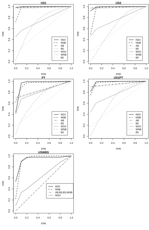
F P R=F P/(F P +T N) (6) whereT P,F P,T N andF Ndenote the number of true positives, false positives, true negatives and false negatives. The receiver operating characteristic (ROC) curve shows the performance of a two class classifier across the range of possible threshold (D) values, plottingF P R(x-axis) versusT P R(y-axis) [7]. The global accuracy is given by the area under the curve (AU C=R1

0 ROCdD). A random

classifier will have an AUC of 0.5, while the ideal value should be close to 1.0. With the incremental retraining procedure, oneROCis computed for eachbi+1

batch and the overall results are presented by adopting the vertical averaging

ROC (i.e. according to the F P R axis) algorithm presented in [7]. Statistical confidence is given by the t-student test [8].

3

Experiments and Results

We tested all methods from Section 2.2 in all datasets from Table 2 and using a retraining evaluation with a batch size of k = 100 (a reasonable value also

adopted in [12]). The obtained results are summarized as the mean of all test sets (bi+1,i∈ {1, . . . , n−1}), with the respective 95% confidence intervals and

shown in Tables 3 and 4. To increase clarity, we only show the best blacklist (B6) in Table 3. In the tables, the best values are in bold, while underline denotes a statistical significance (i.e. p-value<0.05). In Table 3, the significance was computed for a paired t-test comparison of the network-level approach against AB and the corresponding bag-of-words method (e.g. NSV vs AB and WSV). In Table 4, the paired t-test is performed against the second best blacklist (B4). Under the AUC metric and for all setups, the NSV method is the best choice and the obtained results are of high quality (from 95.3% to 99.8%). The NNB is the second best filter for the last three datasets. It is also interesting to notice that both NSV and NNB are robust to a geographic spread of the ham origin, since there is only a slight decrease (0.4 and 0.8 pp) when comparing US2 and US1 filtering performances. For WSV, the detection capability is higher when there is Portuguese ham (PT and US1PT). This was an expected behavior, since most spam is written in English. The bag-of-words performances decrease substantially for the last setup, showing that the spam that is not detected in blacklists is more difficult to classify based on content. However, our network-level based methods still obtained high AUC values, around 95%. When using the same inputs, the SVM algorithm is always better when compared with NB, with an average improvement of 1.2 pp for the network-level features and 9.7 pp for the bag-of-words attributes.

Table 3.Comparison among the main filters (AUC test set results, in %)

setup B6 AB WNB WSV NNB NSV US1 98.0±0.898.9±0.573.0±4.775.8±2.298.7±0.699.8±0.2 US2 98.1±0.798.9±0.665.4±2.777.0±2.397.9±0.899.4±0.5 PT 83.9±4.589.0±3.471.4±7.582.1±5.195.6±1.597.3±1.6 US1PT 94.5±0.996.3±0.868.4±3.478.2±2.098.2±0.599.2±0.4 USWBS 50.0±0.050.0±0.050.1±0.363.6±7.694.7±3.495.3±3.6

Table 4.Blacklist filter performances (AUC test set results, in %)

setup B1 B2 B3 B4 B5 B6 B7 B8

US1 87.6±1.280.2±1.880.8±1.687.7±1.258.7±1.198.0±0.874.3±2.667.1±2.6

US2 88.7±1.280.3±2.079.4±2.088.9±1.259.2±1.098.1±0.774.0±2.667.5±3.0

PT 76.0±3.874.7±2.169.1±3.778.0±4.259.0±3.083.9±4.565.5±3.063.0±4.5

Regarding the blacklist comparison (Table 4), B6 is clearly the best filter. Overall, the second best DNSBL is B4, followed by B1. For all setups, three blacklists (B5, B7 and B8) are outperformed by the WSV model. B5 is the worst filter, with no average AUC value above 60%. For all DNSBLs except B5, the worst performance is achieved for the Portuguese dataset (PT). This outcome was expected, since the tested blacklists are international and thus may fail in mapping more country specific spam.

The full ROC analysis is given in Figure 5. To increase clarity, we only selected the best and worst blacklists (B6 and B5). The ROC curve allows the definition of different filtering profiles, according to the user needs. In the studied datasets, the blacklists never output a false positive. Thus, for B6 and AB, the TPR values are high when FPR is zero. For the spam domain, this is an important point of the ROC curve, since often the cost of losing normal e-mail (F P) is much higher than receiving spam (F N). This is particularly true if the email client action is set to delete messages marked as spam. For this decision point, AB, followed by B6, are the best filters, except for US1 and USWBS, where NSV is the best option. For larger admissible values of FPR, NSV gives the best TPR values. It should be noted that for some users, this is an interesting scenario, as the cost of receiving spam can also be high, due to an higher vulnerability to phishing attacks, viruses or online fraud, while not all ham is important. Since often email clients move messages marked as spam to a different folder, false positives could still be read by the user.

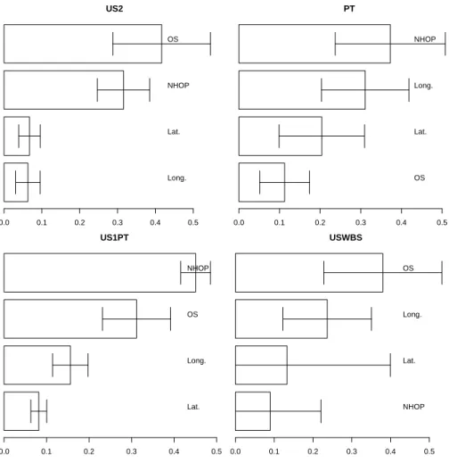
The average network-level feature importances for NSV are plotted in Figure 6. The bar plots show theRa values, while the whiskers denote the 95%

confi-dence intervals. The US1 importance bars are not shown, since they are similar to US2. All four attributes contribute to the model, although their relative influ-ences vary. For example, the operating system (OS) is the most relevant feature for the US datasets, although it is the least important input for PT. On the other hand, the length of the message path (NHOP) is most relevant attribute for PT and US1PT.

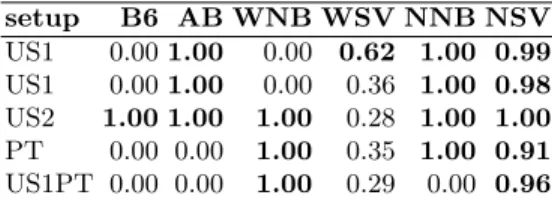
To study the filtering vulnerability to phishing email attacks, we searched within the datasets for spam messages asking for user password details (e.g. related to a bank online account). Five messages were found and the respective spam probability predictions (p(s|xj)) are shown in Table 5. The first column of

the table shows the dataset that contained such messages. Although the number of examples is not enough for a more definitive conclusion, the results seem to favor the network-level based methods. For a decision threshold ofD= 0.5, NSV detects all attacks, while NNB predicts four. The less robust methods are B6 and WSV.

4

Conclusions

In this work, we proposed a new spam filtering approach that is based on four network-level attributes: message path length in terms of number of routers (NHOP), geographic coordinates (i.e. latitude and longitude) and operating

sys-Table 5.Filter responses to phishing messages (values above 0.5 are inbold) setup B6 AB WNB WSV NNB NSV US1 0.001.00 0.00 0.62 1.00 0.99 US1 0.001.00 0.00 0.36 1.00 0.98 US2 1.00 1.00 1.00 0.28 1.00 1.00 PT 0.00 0.00 1.00 0.35 1.00 0.91 US1PT 0.00 0.00 1.00 0.29 0.00 0.96

tem of the sender. We tested two data mining (DM) classifiers, Naive Bayes (NB) and Support Vector Machines (SVM) and also targeted two countries from differ-ent contindiffer-ents and with differdiffer-ent main languages (i.e. U.S. and Portugal). Since our network-level properties are not currently monitored by filtering systems, we created and developed a new spam repository, called spam telescope. This repository includes real legitimate (ham) and non legitimate (spam) messages. The ham was collected from several mailing lists, while the spam was captured from email traps (fake addresses advertised through the Web). Several experi-ments were carried out, where a realistic mixture of spam and ham was used to simulate distinct user profiles.

When comparing with Content-Based filters (CBF), i.e. bag-of-words, and eight DNS-based Blackhole Lists (DNSBL), the NSV method (SVM fed with the four network-level features) obtained the best discriminatory performance, with high quality results (from 95.3% to 99.8%). The NSV method requires much less computation than the respective bag-of-words filter. Also, in contrast with the blacklist methods, it does not require communication with other servers, since the free geographic IP database that we used can be installed locally. Moreover, preliminary results suggest that NSV is more robust to phishing email attacks.

Based on the achieved results, we advise the use of the NSV filter, which provides a high true positive rate (i.e. detects most of the spam). To reduce false positives (i.e. ham marked as spam), this method could be used after a first phase blacklist filtering. Yet, for an effective blacklisting, it should be considered a careful DNSBL server selection or (even better) use of multiple DNSBLs.

Spammers and anti-spammers are in a continuous struggle. The research community has devoted a large attention to improve CBF. Yet, as argued in [15], spammers can easily change content to confuse CBF filters but network-level properties are more persistent in time. For example, a large portion of current spam comes from botnets. Most spammers are greedy and want a mas-sive distribution of spam, thus they do not care about the location of a given controlled machine. Furthermore, some operating systems (e.g. Windows) are more vulnerable to botnet control by malicious software. Hence, we believe it is more difficult for spammers to surpass network-level based filters. As future work, we intend to enlarge the experiments to other countries (e.g. Spain). Also, we wish to deploy the proposed models in real email clients (e.g. Thunderbird) to gather more feedback.

Acknowledgments

This work is supported by FCT grant PTDC/EIA/64541/2006. We also wish to thank David Manzieres for supporting Mail Avenger.

References

1. R. Beverly and K. Sollins. Exploiting transport-level characteristics of spam. In

5th Conference on Email and Anti-Spam (CEAS), 2008.

2. R. Bilisoly. Practical text mining with Perl. Wiley Publishing, 2008.

3. E. Blanzieri and A. Bryl. A survey of learning-based techniques of email spam filtering. Artificial Intelligence Review, 29(1):63–92, 2008.

4. V. Cherkassy and Y. Ma. Practical Selection of SVM Parameters and Noise Esti-mation for SVM Regression. Neural Networks, 17(1):113–126, 2004.

5. P. Cortez, A. Cerdeira, F. Almeida, T. Matos, and J. Reis. Modeling wine prefer-ences by data mining from physicochemical properties. Decision Support Systems, 47(4):547–553, 2009.

6. P. Cortez, C. Lopes, P. Sousa, M. Rocha, and M. Rio. Symbiotic Data Mining for Personalized Spam Filtering. InProceedings of the IEEE/WIC/ACM International

Conference on Web Intelligence (WI-09), pages 149–156. IEEE, 2009.

7. T. Fawcett. An introduction to ROC analysis.Pattern Recognition Letters, 27:861– 874, 2006.

8. A. Flexer. Statistical Evaluation of Neural Networks Experiments: Minimum Re-quirements and Current Practice. InProceedings of the 13th European Meeting on

Cybernetics and Systems Research, volume 2, pages 1005–1008, Vienna, Austria,

1996.

9. B. Leiba, J. Ossher, VT Rajan, R. Segal, and M. Wegman. SMTP path analysis.

InProceedings of the Second Conference on E-mail and Anti-Spam (CEAS), 2005.

10. H.T. Lin, C.J. Lin, and R.C. Weng. A note on Platts probabilistic outputs for support vector machines. Machine Learning, 68(3):267–276, 2007.

11. MAAWG. Email Metrics Program: The Network Operators’ Perspective. Report #10 – third and fourth quarter 2008, Messaging Anti-Abuse Working Group, S. Francisco CA, USA, March 2009.

12. V. Metsis, I. Androutsopoulos, and G. Paliouras. Spam Filtering with Naive Bayes

– Which Naive Bayes? In Third Conference on Email and Anti-Spam (CEAS),

2006.

13. B. Nelson, M. Barreno, F. Chi, A. Joseph, B. Rubinstein, U. Saini, C. Sutton, J. Tygar, and K. Xia. Exploiting Machine Learning to Subvert Your Spam Filter.

In1st Usenix Workshop on Large-Scale Exploits and Emergent Threats, pages 1–9.

ACM Press, 2008.

14. R Development Core Team.R: A language and environment for statistical comput-ing. R Foundation for Statistical Computing, Vienna, Austria, ISBN 3-900051-00-3, http://www.R-project.org, 2009.

15. A. Ramachandran and N. Feamster. Understanding the Network-Level Behavior of Spammers. In ACM, editor,SIGCOMM’06, pages 291–302, 2006.

16. X. Wu, V. Kumar, J. Quinlan, J. Gosh, Q. Yang, H. Motoda, G. MacLachlan, A. Ng, B. Liu, P. Yu, Z. Zhou, M. Steinbach, D. Hand, and D. Steinberg. Top 10 algorithms in data mining. Knowledge and Information Systems, 14(1):1–37, 2008.

0.0 0.2 0.4 0.6 0.8 1.0 0.0 0.2 0.4 0.6 0.8 1.0 US1 FPR TPR NSV NNB AB B6 WSV WNB B5 0.0 0.2 0.4 0.6 0.8 1.0 0.0 0.2 0.4 0.6 0.8 1.0 US2 FPR TPR NSV NNB AB B6 WSV WNB B5 0.0 0.2 0.4 0.6 0.8 1.0 0.0 0.2 0.4 0.6 0.8 1.0 PT FPR TPR NSV NNB AB B6 WSV WNB B5 0.0 0.2 0.4 0.6 0.8 1.0 0.0 0.2 0.4 0.6 0.8 1.0 US1PT FPR TPR NSV NNB AB B6 WSV WNB B5 0.0 0.2 0.4 0.6 0.8 1.0 0.0 0.2 0.4 0.6 0.8 1.0 USWBS FPR TPR NSV NNB AB,B6,B5,WNB WSV

US2 0.0 0.1 0.2 0.3 0.4 0.5 Long. Lat. NHOP OS PT 0.0 0.1 0.2 0.3 0.4 0.5 OS Lat. Long. NHOP US1PT 0.0 0.1 0.2 0.3 0.4 0.5 Lat. Long. OS NHOP USWBS 0.0 0.1 0.2 0.3 0.4 0.5 NHOP Lat. Long. OS