3D CFD-analysis of conceptual bow wings

3D CFD-analysis of

conceptual bow wings

P A U L N I E L S E N p a u l n i @ k t h . s e 0 7 0 7 - 3 8 4 4 9 6

Master Thesis Ver. 0.1 KTH Center for Naval Architecture February 2011

A

As a small step towards their long-term vision of one day producing emission free vessels, Wallenius em-ployed, in 2009, Mårten Silvanius to carry out his master thesis for them in which he studied five different concepts to reduce the overall fuel consumption using wind powered systems. The vessel on which his study was performed is the 230 m LCTC vessel M/V Fedora. One of the concepts studied was the bow wing which is thought to generate enough force in the ship direction to profitably reduce the overall wind resistance. His calculations showed that the wing would be the preferred method of the different concepts studied since it was determined cheapest to build, had good payback, had good global drag reducing ef-fects and had a predicted performance of a reduction in fuel cost between 3-5% on a worldwide route. This thesis is conducted mainly to verify the results of Silvanius numerical study. The method chosen is to perform a fully viscous 3-D CFD study on the entire flow around the above water portion of the ship in full scale. A 3-D model is created and the wing is placed using suggestions given by Silvanius.

One major limitation in this project was the computational capacity available at the time this thesis was conducted. In order to run some of the viscous grids created the grids had to be severely coarsened. This had a negative impact on the reliability on some of the results.

Since it has been difficult to obtain satisfactory solutions, no work has been done to optimize the shape and position of the wing.

Nevertheless, one it has been shown that the wing does in fact affect the resistance in a positive way, however nowhere near as much as predicted by Silvanius. This effect needs to be further determined through further calculations, both using CFD and also through experimental wind tunnel testing where alternatives to the wing profile should be tested, e.g. replacing the wing with a vortex generator to further delay the point of separation.

A

First and foremost I would like to thank one of my supervisors in this project, Maximilian “Mio” Tomac at KTH, without whom I would be completely lost in the jungle that is CFD.

I would also like to thank my other supervisors, Karl Garme (KTH) and Mikael Huss (Wallenius), for their contributions during the different stages of this thesis.

Furthermore I would like to acknowledge the support that Exjobbsgruppen has given me, especially one member, Carl Hedgren, for his spontaneous disruptions and rewarding discussions which in no way helped me forward in the project but were nevertheless highly appreciated.

Lastly I also would like to express my gratitude to the staff at the department of Ship design at Wallenius Marine for providing me with a pleasant working environment during my short stay at their offices at the start of this project.

C

I. Abbreviations ... 6

II. Nomenclature ... 7

1. Introduction ... 9

1.1. Purpose and Objective ... 9

1.2. Method ... 9

1.2.1. Basic CFD Procedure ...10

1.2.2. Software ...10

1.3. Resource limitations ...11

2. Studied ship & the bow wing ...11

2.1. The investigated setup ...13

3. Numerics ...13

3.1. Basic ship theory: Silvanius approach ...13

3.2. The governing equations...15

3.2.1. Steady state calculations ...16

3.2.2. Time accurate calculations ...16

4. Aspects regarding the CFD process ...16

4.1. 3D-modeling ...16 4.2. Discretization ...18 4.2.1. Mesh type ...19 4.2.2. Mesh requirements ...19 4.2.3. Mesh method ...20 4.2.4. Euler mesh ...22 4.2.5. RANS mesh ...22 4.2.6. Mesh quality ...24 4.3. CFD solver process ...26

4.3.1. The input file ...26

4.3.2. Boundary conditions ...30

4.3.3. Preprocessor ...30

4.3.4. Flow solver ...31

4.3.5. Post-processing ...31

5. The road to convergence and reliable results ...32

5.1. Solution dependency ...32

5.2. The computational domain ...33

5.3. Convergence through comparisons and testing ...34

5.3.1. Numerical alterations ...34

5.3.2. Scaling the speed and density ...35

5.3.3. Grid dependency ...38

6.1.1. Concerning the bow effect ...43

6.2. Effects when adding the wing ...44

6.2.1. Effects on the flow structure ...45

6.2.2. Force generated from wing ...47

6.3. Effects of altering mounting position and sheet angle ...47

7. Conclusions ...49

8. Recommendations ...49

Appendix A – Pressure distribution comparisons ...50

Appendix B – Streamline comparisons ...52

Appendix C – Velocity field comparisons ...55

I.

A

2-D/3-D Two-/Three-Dimensional

BC Boundary Conditions

CFD Computational Fluid Dynamics

CFL Courant-Friedrichs-Levy condition

DES Detached Eddy Simulation

E# Euler mesh

ECMWF European Center for Medium-range Weather Forecasts

FOI Swedish Defence Research Agency (Sw. Totalförsvarets Forskningsinstitut)

GB Gigabyte

GUI Graphical User Interface

IGES Initial Graphics Exchange Specification

KTH Royal Institute of Technology (Sw. Kungliga Tekniska Högskolan) LCTC Large Car and Truck Carrier

LES Large Eddy Simulation

M/V Merchant Vessel

N-S Navier-Stokes

NACA National Advisory Committee for Aeronautics

PLM Product Lifecycle Management

R# RANS mesh

RAM Random Access Memory

RANS Reynolds-Averaged Navier-Stokes equations

Rhino Rhinoceros

RORO Roll-On Roll-Off

RK Runge-Kutta

WB ANSYS Workbench

WT Wind Tunnel

II.

N

Latin symbols Description Unit

AF Projected frontal area of above water portion of ship [m2]

AS Projected side area of above water portion of ship [m2]

Aw Projected area of wing [m2]

B Maximum width of ship [m]

CD 3-D drag coefficient [-]

Cd Non-dimensional force coefficient in ship direction [-]

Cf Skin friction coefficient [-]

CL 3-D lift coefficient [-]

Cl Non-dimensional side force coefficient [-]

Cm Non-dimensional moment coefficient [-]

Cp Pressure coefficient [-]

CX Non-dimensional force coefficient in ship direction [-]

∆CX Difference of the non-dimensional force coefficient in ship direction [-]

CY Non-dimensional side force coefficient [-]

D The heigth of the ship measured from the keel line to weather deck [m]

D Drag force generated by wing [N]

Fi Arbitrary force [N]

H

xA

F _{Aerodynamic force acting on hull in ship direction [N]}

H

yA

F Aerodynamic side force acting on hull [N]

S

xA

F Aerodynamic force acting on wing in ship direction [N]

S

yA

F Aerodynamic side force acting on wing [N]

H

H

F Hydrodynamic force acting on hull [N]

P

H

F Hydrodynamic force acting on propeller [N]

R

H

F Hydrodynamic force acting on rudder [N]

G Function loosely dependant on ln(Re) [-]

k Kinetic energy [J]

k-ω Turbulence model type [-]

L Lifting force generated by wing [N]

L Characteristic length [m]

LOA The overall length of the ship [m]

LPP The length between the ships perpendiculars [m]

n Number of time steps [-]

Pi Arbitrary power [W]

Q Dynamic pressure [Pa]

Re Reynolds number [-]

Re/m Reynolds number over length [m-1_]

T The design draft of the ship [m]

U∞ Magnitude of free stream velocity [m/s]

(ue, ve, we) Free stream velocity components in the (x, y, z) direction [m/s]

uτ Wall friction velocity [m/s]

VA Apparent wind speed [m/s]

VS Ship speed [m/s]

VT True wind speed [m/s]

x Characteristic length [m]

(X, Y) Global coordinates [-]

(x, y) Local coordinates [-]

y Normal distance to nearest wall [m]

Greek symbols Description Unit

α Vertical angle of attack [°]

β Horizontal angle of attack [°]

β Apparent wind angle [°]

βlocal Local apparent wind angle [°]

γ True wind direction [°]

δ Sheet angle [°]

ζ Mounting position of wing measured from the ships centerline [°]

ηship Ship propulsion efficiency [-]

κ Karmans constant, = 0.41 [-]

λ Drift angle [°]

μ Dynamic viscosity [Pa∙s]

ν Kinematic viscosity [m2_/s]

Quantity equivalent to eddy viscosity [m2_/s]

ρ Fluid density [kg/m3_]

τw Shear stress at the wall [N/m2]

1. I

During 2009 Wallenius Marine conducted a project called ZERO (Zero Emission RORO) where a plan was created for how to reach their long-term vision of one day producing emission free vessels. A major part of their vision is the increased exploitation of emissionless sources of energy, such as solar, wave and wind energy. The source in which the largest amount of energy can be extracted is presumed to be from wind [1].

In 2009, Mårten Silvanius conducted his master thesis for Wallenius in which he studied how different wind powered systems could decrease the fuel consumption for a 230 m LCTC (Large Car and Truck Carrier) vessel. The vessel which served as norm was the M/V Fedora (Figure 1) which is a relatively new addition to the Wallenius fleet. This vessel is assumed to operate on a world-wide route, 220 days each year, with an average daily fuel consumption of 56 tonnes/day. The average fuel consumption is based on wind statistics provided by the ECMWF (European Center for Medium-range Weather Forecasts) when going at the ships design speed of 20 knots.

Figure 1. The M/V Fedora [2].

Silvanius studied a total of five different wind powered systems; the Flettner rotor, the wing sail, the kite, the horizontal and vertical axel wind turbine. His studies showed that the preferred system would be to install vertical wings at the bow of the ship as this had a good payback investment, was cheap to build and maintain and had a measurable performance. The results in his thesis [3] showed that the vertical bow wings could save up to 3-5% of the fuel consumption. The potential of these wings are further investi-gated in this thesis.

1.1. PURPOSE AND OBJECTIVE

Silvanius thesis only covered a minor 2-D CFD (Computational Fluid Dynamics) analysis showing the airflow around the bow area (without wings) of the ship. In order to completely understand how bow wings would affect the flow around the entire ship a complete 3-D CFD-analysis is a good start, prefera-bly followed by wind tunnel testing. A 3-D analysis will also be able to take in to account some aspects that were not considered in the 2-D analysis, such as the reduced effect to global drag due to delayed sepa-ration and how the new airflow affects the wake.

The overall goal of this thesis is to determine how large the potential is for a decrease in fuel consumption for a LCTC vessel whilst fitted with bow wings. Furthermore the shape and position of these wings are to be evaluated in order to reach maximum effect. Also, the results from Silvanius thesis are to be verified through this thesis. By performing a complete 3-D analysis of the above water portion of the ship, all the aforementioned objectives can be reached.

1.2. METHOD

The main objective is to analyze the air flow around the above water portion of a LCTC vessel. One me-thod of doing this is to perform a complete 3-D CFD-analysis of the vessel in question. This basically means solving the Navier-Stokes (N-S) equations, which define any single-phase fluid flow [4], using computer software specially developed for these types of problems.

Firstly, a model of the ship without bow wings (later referred to as the naked model) will be created and run through the CFD process (briefly covered below) mainly to be used as reference to the case with wings. Also the results of the naked model will provide information regarding where and in which area of the bow that it would be beneficial to position the wings. Furthermore the results for the naked model will be compared to those from the 2-D calculations performed by Silvanius.

1.2.1. Basic CFD Procedure

For starters a 3-D model needs to be created featuring only the above water portion of the ship in ques-tion, where all details that has insignificant impact on the overall results are removed since these details would only add to the amount of computer work needed further on in the CFD process. One can use any 3-D modeling tool to complete this task providing that the software used is capable of exporting the model in the appropriate file format.

When satisfied with the geometrical 3-D model it needs to be discretized properly to form a volume mesh befitting the case under investigation. Firstly an Euler-mesh is created (used for inviscid Euler calcula-tions) and then run through the flow solver in order to evaluate the quality of the mesh.

For the viscous RANS (Reynolds-Averaged Navier-Stokes) calculations a RANS-mesh is created where prismatic layers are added to the Euler-mesh in order to be able to better resolve for the boundary layer. Thereafter the appropriate method of modeling the turbulence needs to chosen and boundary conditions need to be set along with a number of parameters in order to reach convergence. The residuals and rele-vant results are thereafter visualized and analyzed.

1.2.2. Software

The vessel under investigation is a relatively large object that will require a large number of elements to accurately describe the flow. Also this requires that the dimensions are described as precisely as possible. As of today there exists no software which includes all necessary parts of the CFD process, therefore the job is divided into four kinds of software, each designed to carry out one specific task; 3-D modeling, mesh generating, flow solving and data visualization.

The 3-D model of the hull from the baseline up to the weather deck is provided by Wallenius. The desired superstructures are created in Solid Edge (from Siemens PLM Software) and the wings are created using Rhinoceros (developed by Robert McNeel & Associates and later referred to as Rhino). The main differ-ence between the two programs is that Solid Edge creates solids (as the name implies) and Rhino primarily creates surfaces which can later be made into solids. However, since only the surfaces are going to be meshed it will not matter if the model is solid or only a shell.

Although both programs are equally capable of creating all intended objects on its own, Solid Edge was chosen to create the superstructures as it is easier and quicker to create large blocks whilst the wing was created in Rhino simply because it has a function that can import lines and curvatures from a PDF-file, which greatly simplifies the task of creating an airfoil with exact dimensions and curvatures.

The computational domain and volume net is generated using ANSYS ICEM CFD (later referred to as ICEM), which is a flexible mesh generating tool for the ANSYS Workbench [5]. It is capable of creating large volume or surface meshes with a wide range of shell format variations and mesh generating methods. Although this software is also capable of creating and modifying geometric models, it is not as accurate as software specifically designed for this purpose. The geometric modeling tools are mainly used to patch up and modify existing models created elsewhere that may have been damaged (e.g. disrupted surface connec-tivity, gaps etc.) during the exporting and importing process.

The flow solver used to perform the computations is the Edge-code. Edge is a CFD flow solver for un-structured grids that solves the three-dimensional, compressible RANS equations on hybrid grids. It solves problems in both viscid (using Navier-Stokes equations) and inviscid (using Euler equations which are Navier-Stokes equations simplified) flow on arbitrary elements [6]. Edge was developed by FOI (the Swedish Defence Research Agency) and is one of the leading commercial flow solvers being used.

The governing equations are integrated explicitly towards steady state with Runge–Kutta time integration. Results like pressure distributions and aerodynamical coefficients are obtained and can be graphically

pre-sented in visualization applications such as Paraview. Edge can be used for steady state calculations as well as time accurate ones including manoeuvres and aeroelastic simulations.

Edge is a purely aerodynamic flow solver as it is intended for aircraft calculations. This means that for hydrodynamic calculations one would have to use another flow solver. However since only the above water portion of the ship is under investigation, Edge will be enough to complete the task at hand.

In order to be able to compute several cases (one case being either an Euler or RANS computation, naked or winged model and one specific apparent wind angle) at the same time the computations will be run on a high-performance computer available at KTH (the Royal Institute of Technology) that utilizes parallel computing. Each case is allocated to a node connected to this computer. The computer has a total of 640 nodes [7], where each computer node is allocated 8 GB of RAM (Random-Access Memory).

The results are visualized using ParaView, which is a multi-platform data analysis and visualization applica-tion where one can analyze their data using quantitative and qualitative methods. ParaView is capable of analyzing datasets of all sizes and can therefore be used on supercomputers as well as on laptops [8].

1.3. RESOURCE LIMITATIONS

At the time when this thesis was conducted there was a limit on how fine the mesh could be, or rather how much RAM that was available at computing nodes. The required memory needed is directly propor-tional to the amount of grid points present in the mesh [9], e.g. a mesh containing 5 million grid points would require around 5 GB of RAM. Therefore any mesh used on the high-performance computer needs to contain ≤ 8 million grid points. This criterion is met by most cases except for the RANS-mesh for cas-es where the wing is prcas-esent which contains around 12-17 million grid points.

One effect is that the number of prismatic layers in the RANS-mesh for the winged model had to be re-duced from 50 (as for the naked model) to 30 layers since the addition of the wing significantly increases the total amount of grid points and thusly greatly increases the amount of RAM necessary to handle the model appropriately. Also the entire surface mesh had to be coarsened (as shown in Figure 2) in order to be able to run computations on the high-performance computer.

Figure 2. The surface mesh at the bow as it is for most cases (left) and the coarsened mesh for the winged RANS calculations (right).

Computations will however be done on the original mesh (as well as on a further refined mesh), one case at a time, on a local computer with a greater RAM capacity. Since only one case can be computed at a time only a few selected number of apparent wing angles will be investigated.

2. S

&

The panamax vessel Fedora is chosen to serve as norm for comparative reasons since the same vessel was used in Silvanius studies. With a maximum capacity of 8000 car units (1 car unit = 8.4 m2_{) the M/V}

Fedo-ra makes for one of the largest car carriers in the world [2] and, for Wallenius, it is of primary interest to lower its daily fuel consumption in any way possible. The principal particulars of Fedora can be seen in Table 1.

Table 1. Principal particulars of the M/V Fedora.

[m]

Length over all, LOA 227.80

Length between perpendiculars, LPP 219.30

Breadth, B 32.26

Detpth, D 34.70

Design draft, T 9.50

Projected frontal area, AF 1132

Projected side area, AS 6885

The value of the projected frontal and side areas of the ship are based on only the above water portion of the ship. A blunt body such as this generates a large wind resistance. However the Fedora comes with the characteristic semicircular bow shape which, in Silvanius studies, proved to be advantageous in terms of local acceleration and redirection of the airflow around it (see Figure 3).

Figure 3. Topview of the bow where the different angles are defined [3].

VA is the apparent wind speed and the angle in which it attacks from is the apparent wind angle, β

(meas-ured from the centerline). The local apparent wind angle βlocal refers to the altered apparent wind angle

which comes from the assumed redirection of the airflow due to the bow. The assumption is that as long as β<90° the flow will remain parallel to the hull until separation occurs and that the wind direction only depends on the mounting position, ζ (measured from the centerline), through

90

local . (1)

The angle δ is the sheet angle of the wing and L and D are the resulting lift and drag forces from the wing. Mounting wings at the bow is thought to have mainly three advantages that are to be confirmed with CFD calculations. Firstly, in favorable conditions, the wings are thought to generate a contributing lifting force in the ship direction, large enough to profitably affect the overall resistance of the ship. Secondly the heel-ing moment generated from wheel-ings mounted at the bow is thought to be less than would they be mounted on deck. Lastly it is mentioned but not investigated that the wings improve the airflow around the vessel by delaying the point of separation and thusly reducing the drag.

2.1. THE INVESTIGATED SETUP

Besides calculating the vessel without wing, this thesis primarily focuses on the setup of the wing sug-gested by Silvanius. This setup is presented in Table 2.

Table 2. Wing setup as suggested by Silvanius.

Setup

Mounting position, ζ 20°

Sheet angle, δ 13°

Distance from hull 4 m

Wing profile NACA 6412

Apart from the suggested setup, two other wing positions, 10° and 30° from the centerline, and also one other sheet angle, 20°, was investigated. The calculations were done on a full-scale 3-D model of the ship and the apparent wind angle, β, was taken as every 5° from 0°-45° from the centerline with an apparent wind speed, VA, of 20 knots in every direction.

3. N

This chapter covers the basic numerics used in this thesis. The first section (Section 3.1) loosely covers how Silvanius approached his study through basic ship theory. The objective of this section is to describe how Silvanius results will be evaluated numerically. This is done by first describing shortly how he ap-proached his assignment followed by which aspects are considered in this thesis. The second section (Sec-tion 3.2) discusses the governing equa(Sec-tions and numerical methods of solving them in the CFD process through brief descriptions and only the default methods in the flow solver is mentioned. For more de-tailed information of how the governing equations are derived, how the default numerical methods are composed and also information on other methods available, see [15] or [17].

3.1. BASIC SHIP THEORY:SILVANIUS APPROACH

Basically what Silvanius did was determining at which angle of attack a certain wing profile generated max-imum lifting force, subsequently the effect gained from this force, and then subtracted its component in the ship direction from the total engine power needed to power the ship (which was calculated separately) whilst taking into account for some aspects that affect the total power gained from the wing.

The lifting, L, and drag, D, force of the wing seen in Figure 3 are calculated through

, , w x L w y D L qA C D qA C (2)

where, Aw is the projected area of the wing in the direction of the force, CL and CD are dimensionless 3D

lift and drag coefficients and q is the dynamic pressure which, for incompressible fluids (which is assumed for air due to the relatively low speed of the ship), is calculated

2 2

A V

q (3)

where ρ is the fluid density and VA is the apparent wind speed which is calculated through

2 2

2 cos

A T S T S

V V V V V (4)

and the apparent wind angle, β, is calculated through

2 2 2 1 cos 2 T A S A S V V V V V (5)

where VT is the true wind speed, VS is the ship speed and γ is the true wind direction. All speeds and

an-gles are defined in Figure 4.

The lift and drag forces from the wing are not of primary interest as much as how they each contribute the total aerial resistance in the ships direction. Using the apparent wind direction these forces are trans-lated to form the generated force in the ship direction FxA_S and the side force FyAS (both of which are

defined in Figure 4) through

cos sin sin cos S S xA yA F _D F L (6)

Assuming that the flow is redirected as discussed in the previous chapter the apparent wind angle β in (6) is replaced with the local apparent wind angle, βlocal, as defined in Figure 3. Furthermore, the assumption

provides that the wing will always be attacked from the same angle, the sheet angle δ, and thusly always have the same lift and drag coefficients, CL and CD (determined through an online Java script, JavaFoil

[10]), regardless of the apparent wind angle as long as β<90°.

The aerodynamic force, FA_H(defined in Figure 4), acting on the hull is calculated separately in a similar

fashion as the lift and drag forces in (2) through its components in the side and ship direction

H H xA F x yA S y F qA C F qA C (7)

where again q is the dynamic pressure determined through (3), AF and AS are the projected frontal and

side area respectively of the above water portion of the ship and Cx and Cy are the force coefficients in the

ship and side direction. The values used in Silvanius thesis for the dimensionless coefficients were deter-mined through wind tunnel tests on a 1:200 scale model of the ship in question by DSME at Force tech-nology in Denmark [3].

To translate any calculated force, Fi, into its corresponding propulsion power, Pi, the following equation is

used i S i ship FV P (8)

where ηship is the ship propulsion efficiency set to 0.75.

Figure 4. Definition of forces, variables, angles and coordinate systems [3].

Table 3. Definitions of variables, angles and coordinate systems.

Variable Definition

R H

F _{Hydrodynamic force generated by rudder}

H H

F _{Hydrodynamic hull forces}

P H

F _{Propeller propulsion force}

(X, Y) Global coordinates in which the ship moves

(x, y) Local coordinates

λ Drift angle

The hydrodynamic forces mentioned in Table 3 will not be evaluated any further in this thesis.

The aerodynamic solver is capable of calculating the absolute forces acting on the entire ship, with or without wing, as well as the forces acting on defined sections of the model (e.g. the wing alone, the hull and the superstructures separately). However it does this by first determining the dimensionless force coefficients in the defined directions, i.e. Cx and Cy. The translation in (6) is done automatically in the flow

solver when properly defining the direction of the force coefficients.

This thesis will mainly present results showing the force coefficients and any comparison made will there-fore be a comparison between the coefficients used in Silavnius thesis and those calculated here, the dif-ference being that the force coefficients determined through CFD will contain information on how the wing affected the ships resistance whenever it is present.

3.2. THE GOVERNING EQUATIONS

The core of any CFD application could be to solve either potential equations, Euler equations or the Navier-Stokes (N-S) equations. The N-S describes how the pressure, temperature and density are related for a moving fluid. They comprise of a set of coupled partial differential equations; one continuity equa-tion for the conservaequa-tion of mass, three equaequa-tions for the conservaequa-tion of momentum and one equaequa-tion for the conservation of energy, all of which are time-dependant [16]. Although theoretically possible, these equations are very difficult to solve analytically and are therefore more commonly solved on computers through approximations.

Normally one is only interested in knowing the time-averaged properties of the flow (e.g. mean velocities, mean pressure etc.) and not interested in considering all of the small-scale fluctuations in the atmosphere. Therefore some averaging operators are introduced adding some additional terms to the governing equa-tions which represent the effects of the eddy fluxes created by the scales of motion which have been re-moved in the averaging process [17]. The new system of equations is more commonly referred to as the RANS (Reynolds-Averaged Navier-Stokes) equations and the additional terms are called the Reynolds stresses.

Turbulence models are developed and used in order to predict and approximate these stresses as well as the scalar transport terms and to close the system of mean flow equations so that turbulent flow can be computed using the RANS equations.

By neglecting the viscous effects altogether, the governing Navier-Stokes equations are reduced to the Euler equations, only the continuity equation remains identical [17]. The flow is assumed inviscid and therefore the no-slip condition at the wall boundaries is disregarded.

3.2.1. Steady state calculations

The flow solver used in this thesis (the Edge code) utilizes explicit Runge-Kutta (RK) schemes in order to integrate the governing equations towards steady state. The Runge-Kutta method is a numerical technique to approximate the solution of stochastic differential equations and advances in time in a step-by-step or “marching” manner [17]. The RK method is a multistage method which has the advantage that it does not require any specific starting procedure [22], other than the initial condition required by the differential equation itself, and the extra stages are used to improve the accuracy of the solution and to extend the stability region. A maximum of 10 stages is foreseen in Edge. The default scheme in Edge [15] is a 3-stage, first order accurate scheme which provides good smoothing for both upwind and central schemes. The numerical dissipation is only calculated once in this scheme in the first stage, which reduces the computa-tional cost substantially. The dissipative terms are however stored separately. Convergence is also accele-rated using agglomeaccele-rated multigrids and implicit residual smoothing.

3.2.2. Time accurate calculations

Whenever the case under investigation is determined unsteady in nature, time accurate computations are applied. The flow solver used in this thesis has two methods of carrying out this type of calculations; ex-plicit RK time marching with a global time step or imex-plicit time marching with exex-plicit subiterations [15]. For explicit time accurate calculations a global time step is automatically computed from the minimum local time step in all domains. A RK scheme of at least second order is recommended, however a fourth order scheme is default when explicit time accurate calculations are applied. Explicit calculations are not compatible with the convergence acceleration methods used for steady state calculations, such as multigrid methods or residual smoothing. Explicit calculations have however not been used in this thesis when time accurate calculations have been applied.

Instead implicit time accurate calculations have been used (since this is the default method when switching to time accurate calculations). For these calculations the domain has been divided into a number of user defined real time steps, within which the set of governing equations are solved through explicit RK time marching through a number of subiterations for each real time step. The default scheme for implicit time marching in the flow solver is a second order accurate backward difference scheme which provides good smoothing also for large implicit time steps [15].

4. A

CFD

This chapter describes the CFD-process for this investigation. The first two subchapters (Sections 4.1 and 4.2) cover the modeling and discretization process and the final subchapter (Section 4.3) covers the Edge process. However this section only describes a general approach which was done in the initial stage of this project when the flow calculations were just started. Alterations to this approach is covered in the follow-ing chapter (Chapter 5) where methods to improve convergence are discussed and how this affected the model in this thesis.

4.1. 3D-MODELING

A complete model comprising of the hull (shown in yellow in Figure 5) from the design draft to the weather deck of the ship was provided by Wallenius. Added to the model are the superstructures (shown in blue in Figure 5) that are necessary in order to gain a satisfactory understanding on how the airflow behaves.

Figure 5. The 3D model of the ship showing the hull (yellow) and the added superstructures (blue).

Note that all minor details, e.g. antennas and railings, have been removed (compare the model in Figure 5 with the ship depicted in Figure 1). The dimensions were taken from a detailed general arrangement of the vessel provided by Wallenius. The wing is added with a NACA 6412 profile at three different mounting positions, ζ; 10°, 20° and 30° from the centerline, at a distance of 4 m from the hull (also a suggestion from Silvanius). It is not in any way connected to the hull in the model as presented in Figure 6. The rea-son for this setup is that it is not known how the wings will be connected if they are realized and that it would be sufficient this way to at least determine if it is a feasible solution.

Figure 6. The wing (purple) shown "floating" in the air at a position of 20° from the centerline.

The models are thereafter exported in the IGES-format (Initial Graphics Exchange Specification) and imported to ICEM where some further reparations and alterations are done. It is very common that de-fects in the geometry occur during this process. Such dede-fects could be gaps, overlaps and discontinuities between surface patches [11]. As can be seen in Figure 7 a surface patch on the port side of the lower aft section of the hull (right) and the entire weather deck (left) had to be recreated in ICEM as it was lost during translation.

Figure 7. Defects on the model after importation.

Another side effect of the conversion is that multiple points, curves and surfaces occupying the same space may occur and at least the excess curves and surfaces need to be cleaned up (i.e. removed) since this could affect the discretization process and computations later on.

The vessel is oriented so that the point of origin is placed at the front most tip of the bulb and the coordi-nate system is similar to that of the flow solver. The orientation can be seen in Figure 5.

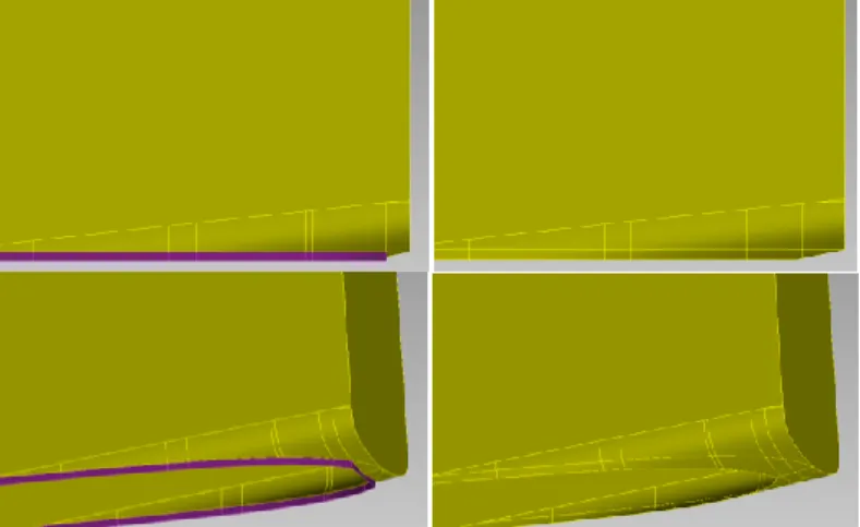
A vertical plane (shown in purple in Figure 8) is then added in ICEM at the lower aft section of the hull. This area has a narrow angle against the “waterline” where the hull is cut and would have required a large amount of small elements to properly reproduce the geometry in this area and since this area is not as important as other areas of the hull (e.g. the frontal area) and there is a limit on how many elements that may be used, the vertical plane was added.

Figure 8. The vessel with (left) and without (right) the vertical plane (purple).

Lastly the computational domain (or rather the farfield boundaries) is created (see Figure 9). The size of which has to be large enough as not to have any influence on the future computations [11]. The domain is shaped like a flat cylinder with a height of 500 m (i.e. ~2LOA) where the ship is centered on the lower

surface which is later defined as the symmetry plane. Initially two different radii were created to study whether or not this would have an effect on the results. These are 5.5LOA and 8.5LOA, later referred to as

5L and 8L respectively. The volumetric mesh is assigned to a point created between the upper surface of the farfield and the symmetry plane (marked as FLUID in Figure 9).

Figure 9. The farfield boundaries (green) and the symmetry plane (purple).

When satisfied with the geometries the discretization process can take place. 4.2. DISCRETIZATION

The objective of discretization is to divide the physical space where the flow is to be computed into a large number of geometric elements called grid cells [11] inside which the governing equations are solved for each element. The different geometric element types available in ICEM are presented in Figure 10.

Figure 10. The different element types; a) triangle, b) quadrilateral, c) tetrahedron, d) hexahedron, e) prismatic and f) pyramid.

Triangular and quadrilateral elements are used in 2-D grids and also on the surface mesh of a 3-D grid. The other elements presented in Figure 10 are used in volume meshing in 3-D grids.

4.2.1. Mesh type

Basically there exist two types of grids; structured and unstructured grids. Structured grids are characte-rized by regular connectivity that can be expressed by a two or three dimensional array which decreases the storage requirement and makes for efficient solver algorithms. Structured grids are restricted to quadri-lateral elements in the surface mesh and hexahedral elements in the volume, an example of a structured grid is shown in Figure 11. A well designed structured grid gives a solution of high accuracy, however the process of generating such a grid is a tedious task (and can take months when dealing with complex geo-metries [9]).

Figure 11. Example of a structured grid.

Unstructured grids however could comprise of all elements shown in Figure 10 (in these cases the grid is more commonly referred to as a mixed or hybrid grid), but mostly they only consist of triangular elements in the surface mesh and tetrahedrons in the volume. The elements have no particular ordering and are placed in an irregular fashion, as shown in Figure 16. This type of grid is the most common in commercial solvers today. Due to the irregularity of the grid distribution the neighborhood connectivity of the differ-ent cells must be explicitly stored which in turn requires significantly more storage space than for struc-tured grids. The generation process can be highly automated and offers high flexibility when dealing with local refinements of the grid without disturbing the overall grid distribution. Mainly for these reasons plus the somewhat complex geometry of the case, an unstructured grid is chosen for this thesis.

4.2.2. Mesh requirements

When creating a mesh there are some aspects that need to be considered since the future results highly depend on the quality of the grid. Both numerical stability and accuracy could be affected by a poor quali-ty grid [9]. Naturally the resolution should be as high as possible, but higher resolution costs more in computing resources and generates slower turnaround times. Primarily there should be no gaps in the grid or overlapping of elements. Furthermore grid points should be clustered around areas of interest such as regions of large gradient (e.g. boundary layers, separation points and shocks), areas where one could ex-pect changes in pressure and also around sharp corners or curves.

a)

c) d)

e) _f)

Also the transition from small to large elements should be smooth so that there are no abrupt changes in the volume of the grid cells. Areas of low interest could have relatively large elements so as to keep the total number of elements to a minimum. When present there should be no large kinks in the grid lines of quadrilateral and hexahedral elements as this could lead to a significant increase in numerical errors [11]. Lastly one needs to make sure to check orientation of the cell faces so that they are normal to the flow gradient.

4.2.3. Mesh method

A typical approach is to start by specifying the global maximum element size allowed to exist in the entire domain. This number is usually quite large in order to minimize the amount of elements needed to fill the entire computational domain. For this project the global element size is set to 200 meters. Obviously this is too large to properly reproduce the geometry of the ship, thus one need to specify element parameters for each surface on the ship. One can also specify element parameters on the curves, but it is not neces-sary to do this on every curve present. The elements sizes on the ship ranges from 0.05 m at the bulb to 4 m on the large horizontal surfaces on the superstructures and hull sides. The element sizes on the wing ranges from 0.01 m on the leading and trailing edges to 0.2 m on the sides.

Figure 12 shows the different element parameters on the ship, unless specified otherwise the curves and surfaces have a maximum element size specification of 0.5 m.

Figure 12. Element parameters on the ship, units are in meters.

For every curve and surface one can also specify a parameter denoted as tetra width. This ensures that the element size for the curve or surface in question does not increase in size until a number of tetrahedron, corresponding to the tetra width, away from the said curve or surface. As seen in Figure 12 this is only applied on the ship where a higher resolution is necessary; along the upper frontal edge of the bridge, bow upper and frontal lower edges, the midline from the weather deck all the way down to the bulb and along the edges at the aft. For the wing on the other hand a tetra width is applied on every surface as well as the leading and trailing edges, the result of which can be seen in Figure 16.

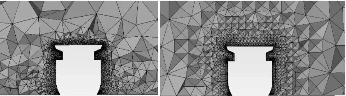
It is also possible to create or manipulate a mesh density volume in areas that are not adjacent to the geo-metry (e.g. the wake of an airfoil). This is done by creating what ICEM calls a mesh density (later referred to as a density field), shaped like a polyhedral (a rounded cylinder), in which one can prescribe a local max-imum element size. For comparative reasons one such polyhedral is created surrounding the entire vessel, with a maximum element size of 3 m within the density field, in order to create a denser mesh close to the vessel. The density field is presented in Figure 13. The presence of a density field of this size naturally increases the number of elements significantly (see Table 5).

1 0.5 along edge, tetra width = 3 0.1 on vertical plane 0.1 4 3 1 0.5 along edge, tetra width = 3 0.05-0.1 along midline, tetra width = 5 1 4 0.4 2 0.4 along edges, tetra width = 3 0.05 at bulb 0.6 0.8 1

Figure 13. Comparison of the volume mesh with (bottom) and without (top) a density mesh.

Prior to choosing generation method one must decide whether or not it should be patch dependent or independent. Patch dependent meshing creates a series of loops which are automatically defined by the boundaries of surfaces and/or a series of curves. The patch independent option on the other hand uses the geometry to associate the faces of the boundaries of the mesh to the regions of interest, thusly ignor-ing gaps, overlaps and other defects that would otherwise be problematic when generatignor-ing a mesh.

It is also usually slower than the patch dependent option. The choice is highly connected to the geometry appearance and quality. For complex geometries and geometries of poor quality (e.g. regarding surface representation etc.) it is recommended to choose the patch independent option [13].

There are several mesh generation methods available in ICEM. For unstructured meshes there are three methods to choose from; the Octree, Delaunay and Advancing front method.

The quickest and most robust method used throughout most of this thesis is the Octree method which is the only method that does not require an existing surface mesh in order to compute, thus saving time not having to do surface and volume mesh separately. The Octree method ensures refinement of the mesh where specified by the user and maintains larger elements where possible, allowing for faster computation. It starts out with a root tetrahedron covering the entire geometry and then subdivides it into eight tetrahe-drons which in turn are each divided into eight new tetrahetetrahe-drons and so on until all element size require-ments are met. The default subdivision ratio is a factor of 2 [13], meaning that elerequire-ments sharing an edge or face do not differ in size by more than a factor of 2, however in some areas it is preferred to specify a lower ratio (in ICEM this is referred to as the height ratio for a specific curve or surface) so that the changes in volume do not increase too rapidly.

One other method of generating a mesh was also used for comparison, namely the Advancing front. This method generates triangles by marching a front of free sides into the unstructured volume domain. The initial front is created by the prescribed boundary edges according to the element parameters previously determined for every surface, therefore it needs an existing surface mesh in order to operate. By extending this initial front, new triangles are created by using existing nodes or creating new ones. The front is the-reafter updated once the new element is created in order to reflect changes due to this creation. This process continues until all sides in the front are removed and the domain is meshed.

Figure 14. Comparison between the Advancing front (left) and the Octree method (right).

The advancing front method shows a higher refinement close to the ship but with a faster increase in element size. Both methods result in a satisfactory overall grid distribution, however with relatively large volume steps away from the ship. This could affect the solution reliability. This however can only be in-vestigated once they have gone through the flow solver.

4.2.4. Euler mesh

The unstructured Euler-mesh consists only of triangular elements on the surfaces and tetrahedrons in the volume. All surface meshes as well as volume meshes are generated using the robust Octree method with patch independency. The Euler-mesh is used for the inviscid Euler calculations. These are done in order to check the behavior of the surface mesh (e.g. no unexpected pressure spikes in unexpected areas), which later will be used to generate the RANS-mesh, and also to give a hint of where one may expect pressure gradients, where (if possible) the mesh needs further refinement and where the end results may land. In-itially the grid was much coarser than is presented in Figure 12 and was refined after having it run through an Euler calculation. Table 4 shows a grid comparison between the different Euler grids created.

Table 4. Grid comparison between the different Euler meshes.

Mesh nr. Farfield radius position, ζ Mounting Total elements [x106_]

Number of nodes [x106_] E1 5L - ~3.3 ~0.58 E2 -||- 20° ~18.8 ~3.23 E3 8L - ~3.3 ~0.58 E4/E5/E6 -||- 10°/20°/30° ~18.5 ~3.17 4.2.5. RANS mesh

Using the surface mesh produced for the Euler-mesh, the RANS-mesh is created by extruding prismatic and quad elements from the surface elements as shown in Figure 16. This procedure is done in order to ensure that no information is lost regarding the boundary layer due to poor resolution [12]. There are several ways to go by when extruding prisms in ICEM. The typical approach is to specify the growth law and at least three of the following parameters; the initial height of the first layer, the total amount of layers present, the prism growth ratio and the total height of the prismatic layers.

The growth law determines the height of each particular layer given the previously mentioned parameters. Three different laws are available in ICEM; the linear, exponential and WB-exponential growth law (this is the exponential growth law as defined in ANSYS Workbench [13]) and Figure 15 shows how the prism layers are extruded with the different growth laws.

The initial height is directly connected to the dimensionless viscous wall distance, y+_{, which is defined as}

yu

y

where y is the normal distance to the nearest wall, ν is the kinematic viscosity and u is the wall friction velocity which in turn is defined as

1 2

W

f

u U C (10)

where τW is the shear stress at the wall, ρ is the fluid density, U∞ is the free-stream velocity, Cf is the skin

friction coefficient which is calculated, using turbulent boundary layer theory for a flat plate at zero inci-dence [18], through 2 ln Re 2 ln Re f x x C G (11)

where the quantity 0.41 is the Karman constant, G ln Re_x is a function which is weakly dependant on ln Rex and is usually set to G = 1.5 and Rex is the Reynolds number for a characteristic length x. The

turbulent Reynolds number is calculated using the full length of the ship, i.e. x = LOA, through

Re_x U x (12)

where ρ is the fluid density and μ is the fluids dynamic viscosity.

A simpler way of calculating the viscous grid spacing is used through an online Java script [19] which uti-lizes the same theory mentioned above.

At least 5-10 grid points should be within y+_{=20 and the initial layer should be within y}+_{=1 [9] in order to}

properly catch all details in the flow inside the boundary layer. The number of prismatic layers is defined by the user and is typically between 30-50 layers within the boundary layer. One method is to extrude all desired layers at once, however since the element sizes vary a lot on the ship this proved to have undesira-ble results in the prismatic layers, also extruding all layers at once can require much computational time when dealing with a large amount of elements. A more robust approach was used where the initial height and total height were left floating (i.e. varying along the surface of the ship) and only five thick layers were initially extruded (see Figure 16) using the exponential growth law and in a later step each layer is split into the desired amount of layers and the grid points redistributed to better satisfy the desired initial height and growth ratio. Furthermore prismatic elements are capped off by pyramids in areas where the quality of the element would otherwise be to poor.

Figure 16. Horizontal cut-plane of the volume mesh surrounding the wing showing the prismatic layers and the result of the tetra width parameter.

All viscous grids created are listed and compared in Table 5. Common for all viscous meshes is that they all have the larger farfield radius, i.e. 8.5 LOA, and that they have been created using patch independent

meshing.

Table 5. Grid comparisons between the different RANS meshes.

Mesh nr. position, ζ Mounting Mesh Method Misc. Prism layers Total elements [x106_]

Num. of nodes [x106_] R1 - Robust Octree - 50 ~13.0 ~5.8 R2 20° -||- - 50 ~33.9 ~12.1 R3/R4/R5 10°/20°/30° -||- Coarsened mesh 30 ~22.2 ~7.7 R6 20° -||-Coarsened mesh with sheet angle, δ=20° 30 ~22.0 ~7.0

R7 - Advancing front Density _field 50 ~15.6 ~6.4

R8 20° -||- -||- 50 ~41.5 ~17.1

Note that both mesh R2 and R8 are too large to be computed on the supercomputer and thusly only one apparent wind angle can be calculated at a time. Therefore only a selected number of measure points are calculated for these meshes.

4.2.6. Mesh quality

In order to avoid any numerical problems further on in the CFD process, where the meshes will be run through the flow solver, it is most desirable to have mesh with high quality. This decreases the chances for divergences due to poor mesh quality. Depending which type of element is considered, ICEM calculates the quality of the element differently. A listing of the different methods for the elements used in this project is presented in Table 6.

Table 6. Quality calculation methods for the different element types [13].

Element type Quality calculation method Value Triangle The minimum ratio of height to

base length of each side of the element

Normalized to 1

Tetrahedron Aspect Ratio of element Value ranges from 0 to 1. 0 indicates no volume in the element and 1 that the element is perfectly regu-lar

Quadrilateral Determinant of element Value ranges from -1 to 1 where negative values indicates inverted element, 0 indicates element dege-nerates and 1 a perfectly regular element

Pyramid

-||-Prismatic Minimum of the determinant

and warpage of the element. Warpage is normalized to a factor between 0 and 1 where 0 indicates a warpage of 90° and 1 a warpage of 0°

The determinant is calculated as the ratio of the smallest and largest determinant of the Jacobian Matrix where the determinant is computed at each node of the element.

The aspect ratio is calculated as the ratio between the radius of an inscribed sphere and a circumscribed sphere for each element, as shown in Figure 17.

Figure 17. Definition of the aspect ratio for tri and tetra elements [13].

The warpage is determined for the quadrilateral faces of a prismatic element by calculating the maximum distortion of said faces.

Typically the quality of the mesh is satisfactory if the quality value is higher than 0.001. However this is no guarantee that things will run unhindered during calculations. The worst element qualities for every mesh created are listed inTable 7. When several different elements are used in the same mesh, the lowest quality is presented.

Table 7. Worst element qualities for the different meshes.

Mesh nr. Worst element quality Element type present

E1 ~0.17 Triangles and tetrahedrons

E2 ~0.17

-||-E3 ~0.12

-||-E4/E5/E6 ~0.11

-||-R1 ~0.0012 Triangles, tetrahedrons, quadrilaterals, prismatic and pyramids

R2 ~0.0022

-||-R3/R4/R5 ~0.0013/~0.0041/~0.0055

-||-R6 ~0.0018

-||-R7 ~0.0011 -||-

If the mesh quality is unsatisfactory (which often is the case, one rarely creates a good quality mesh from the start) there are several tools available in ICEM in order to improve the quality. One such tool is the smoothing operator which can move and/or merge grid points, swap edges and also delete entire ele-ments if needed. It is also possible to choose if all or only some of the different element types are to be smoothed. One can also manually choose specific elements and alter their appearance (e.g. splitting them or moving grid points). If the mesh still is unsatisfactory one should consider changing the mesh generat-ing method or altergenerat-ing the geometry (if possible) to make meshgenerat-ing easier in some areas.

When satisfied with the mesh distribution and quality the mesh is converted into a format compatible with the flow solver.

4.3. CFD SOLVER PROCESS

As previously mentioned the flow solver used for this thesis is the Edge-code. In order to simplify the process of defining different parameters and get a better overview of the case under investigation the code comes with a GUI (Graphical User Interface) called Xedge [14].

Generally there are five steps that need to be taken when making a computation [6]; 1. Set up an input file with relevant parameters for the desired computation. 2. Set proper boundary conditions.

3. Running the preprocessor. 4. Running the flow solver. 5. Post process results.

The last step is done both in Edge and ParaView.

4.3.1. The input file

The general approach is to start by loading a default input file. This file contains all the default values for every parameter which controls the flow solver, preprocessor and other programs within the Edge-code. This is followed by defining case specific parameters in the external flow wizard (as the name suggests, the wizard is primarily used for steady state, external flow calculations). The wizard is divided in two parts where in the first part free stream values of primitive variables (such as the free stream velocities and pres-sure) are related to derived variables, e.g. Mach number, Reynolds number over length (Re/m) and angles of attack etc. The free stream coordinates and angles of attack are defined in Figure 18. It is also possible to define in the first part of the wizard whether or not the computations should be 2-D or 3-D.

Figure 18. Definitions of the angles of attack and the coordinate system in Edge [14].

The components ue, ve and we (the parameter names in Edge for these are UFREE, VFREE and WFREE)

are the free stream velocity components in the x-, y- and z-directions of the magnitude of the free stream velocity, U∞. These are related through the angles of attack through [14]

cos

cos

sin

cos

sin

u

U

v

U

w

U

Throughout all calculations in this thesis the vertical angle of attack ,α, is kept at 0° and only the horizon-tal angle of attack, β, is allowed to vary every 5° between 0° and -45° (one input file is created for every angle and for every mesh). The magnitude of the free stream velocity, U∞, is kept at 20 knots.

The second part of the wizard gives access to crucial parameters for external flow calculations such as whether the calculations are to be viscous or inviscid (INSEUL in Edge). For viscous computations one can further define which turbulence model to use along with other parameters connected to turbulent flow calculations.

A turbulence model is a computational procedure that closes the system of mean flow equations so that a wide variety of flow problems can be solved [11]. The model needs to have a wide applicability, be accu-rate, simple and economical to run in order to be useful in general CFD purposes. Since turbulence is very difficult to model, there exist several different models using different approaches to choose from. The one used for these calculations is the default RANS-based turbulence model for Edge which is a two equation,

k-ω model which uses two additional transport equations that represent the turbulent properties of the flow [9]. In this case one of the equations represents the turbulent kinetic energy, k, and the other one the specific dissipation, ω. It also utilizes an EARSM approximation (Explicit Algebraic Reynolds Stress Mod-el) in which the Reynolds stress tensor is explicitly expressed in terms of velocity gradients and turbulence scales. A more detailed description of this model and several other models available in Edge (e.g. models for detached eddy simulations, DES, and large eddy simulations, LES) and their respective derivations can be seen in [15].

Besides the turbulence model and properties one can further specify in the second part of the wizard the number of multigrids and the amount of full multigrid cycles, initial condition (if one is available, if not this is created in the preprocessor), number of iterations and the logarithmic convergence criterion. The Full Multigrid method (turned on or off with the parameter IFULMG in Edge, default is turned on, i.e. IFULMG = 1) uses a number of coarser grids (defined in Edge by the parameter NGRID, default is 4 grids which is used mostly throughout the thesis) in order to drive the steady state solution on the finest grid faster to steady-state convergence [11]. Calculations are started on the coarsest grid where the approx-imate solution is interpolated to the next finer grids so that a good starting solution is obtained on the finest grid with low numerical effort. The maximum number of iterations on the coarser grids is deter-mined by the parameter NFMGCY, here the default value of 500 iterations is used for all steady-state calculations. IFULMG needs to be turned off (i.e. IFULMG = 0) for time-accurate calculations.

The number of iterations done is determined by the parameter ITMAX (default setting is 1000 iterations, however for most cases in this thesis this number is changed to 4000) and should it turn out that the de-fined number is too low or that the case is unsteady in nature and one wants to switch to time-accurate calculations, it is possible to use the solution from the previous calculation as an initial solution for the new calculation by turning on the parameter INPRES (i.e. =1 or 2 depending on the calculation).

A calculation could be stopped before computing every iteration if the residuals have reduced with an order of magnitude equal to that defined in the parameter RESRED. The default is that computations be stopped when the residuals have reduced with an order of magnitude -5.5, this is however changed for the calculations in this thesis to -10 in order to ensure that every iteration is computed for higher accuracy.

The wizard only provides control over a fraction of the amount of parameters available (more than 100 different parameters), however since these are usually case specific these are, for simple calculations, the only parameters that are changed from the default values. Regarding the numerical parameters, the default settings usually provides with good convergence rates and stable solutions.

Some parameters not considered in the wizard are however changed to fit the calculations for the ship. These are defined in Table 8.

Table 8. Edge parameters altered for calculations on the ship.

Edge

parameter Description Value (default value) Misc.

CFIMSH The input mesh file, must be in the format “.bmsh”.

Name-of-file.bmsh

(Edge.bmsh) Important that a mesh file with this exact name exists in the current working direc-tory

CFIBOC The name of the gener-ated boundary condition file.

Name-of- file.aboc

(Edge.aboc) Name of the boundary condition file later generated by Edge. Changed from default for PDC-purposes in order to distinguish which BC file belongs to which mesh.

INSEUL Determines the

govern-ing equations. 0 = Euler (default) 1 = N-S Can be chosen in the Wizard IFULNS Thin layer approximation

or full N-S. (0 = Thin layer) 1 = Full N-S Only available for viscous calculations. ITURB Turbulence calculation

type (0 = Laminar) 2 = RANS models Only available for viscous calculations. Other available options: 3 = DES models

4 = LES models NPLAYER Number of prismatic

layers 30 or 50 (1) Only for viscous calculations

NPART Number of partitions for

parallel computing 1-8 (1) Varies depending on which computer, or rather on how many processors, the calculations are run

IPOST Post processing options 11

(0) Generates an additional solution file containing information regarding y+_{, Cf}

and other interesting data. For viscous calculations only

IDCLP Direction for lift force coefficient, CL

x, y, z = 0, 1, 0

(0, 0, 1) For plotting purposes, since Edge only plots the lift and drag force coefficients these parameters are switched so that the actual side force in this case is plotted IDCCP Direction for side force

coefficient, CC

x, y, z = 0, 0, 1 (0, 1, 0)

SREF Reference to normalize

force and moment coef-ficients

1132

(1.0) The projected frontal area of the ship is used. Unit [m2_]

As stated above, the parameter IFULNS determines if a thin layer approximation or a fully viscous ap-proach should be applied. The thin layer approximation assumes [21] that for high enough Reynolds numbers the shear layer is very slender and thusly the grid describing it is packed in the surface normal direction whilst being relatively coarse streamwise and therefore only apply viscous terms in the normal derivatives and dropping these terms in the streamwise direction. The full viscous approach is however chosen for this project due to the relatively low speeds (i.e. low Reynolds numbers) being calculated. The parameters presented in Table 8 are basically the same for all calculations.

For low-speed calculations it is recommended to apply preconditioning (controlled by the parameter IPREPA in Edge, default setting is off, i.e. IPREPA = 0) which helps the calculations to reach conver-gence faster. However using preconditioning for the cases in this project led to diverconver-gence or the solution blowing up and therefore was not applied for further calculations.

For time-accurate calculations one must switch on the parameter ITIMAQ, i.e. setting it so that ITIMAQ = 1 for implicit time stepping or = 2 for explicit time stepping. Time-accurate calculations were only done for the inviscid calculations, where implicit time stepping was used, since it would have been too time-consuming to apply time-accurate calculations to the viscous grids (i.e if there had been a need to do so since very few of the viscous calculations indicated that time-accurate calculations were needed).

Implicit time-accurate calculations are computed through a number of global iterations (ITMAX) where each iteration undergoes a set of inner iterations before moving on to the next global iteration. The amount of inner iterations computed are controlled by three parameters; RESTAQ, which controls the convergence criterion on the residuals of each inner iteration (see Figure 19), ITMNAQ and ITMXAQ, which are the minimum and maximum (respectively) amount of inner iterations to be performed. The amount of inner iterations should be large enough to ensure sufficient convergence of the flow variables at each physical time step before moving on to the next [6]. There is no way of telling beforehand how many inner iterations that are needed. The default ITMXAQ amount is 100 iterations and the default ITMNAQ is 3 both of which have remained unaltered whenever time-accurate calculations have been applied. The ITMNAQ value ensures that at least this many iterations will be performed and the ITM-XAQ value forces the calculations to move on to the next global iteration when the amount of inner itera-tions has reached said number.

Figure 19. Principal description of the two convergence criteria, RESRED and RESTAQ.

Another parameter that is crucial for time-accurate calculations and usually very case specific is the para-meter DELTAT which controls the size of the global time step. If the time step is too small, then one might be calculating sound waves, on the other hand if the time steps are too large then the solution might be equivalent to the steady-state solution. The physical time scale usually gives a hint of how large the time step should be [6]. An estimation of the time step is calculated through

L DELTAT

nU (15)

where L is the characteristic length of the object under investigation (in this case, L = LOA), n is the

de-sired amount of time steps and U∞ is the free stream velocity. There should at least be 30-60 [6] time

steps, however when applied for this thesis 100 time steps are used leading to a DELTAT value of ~0.22 sec (default setting for DELTAT is 0.005 sec).

After finishing defining the parameters for the flow calculations, the boundary condition needs to be set.

4.3.2. Boundary conditions

The amount and type of boundary conditions (BC) varies from case to case depending on how the physi-cal geometry is built. Regardless of which BC is chosen there is usually no need to further edit the BC since the default usually are sufficient for all specifications. Four different classes of BCs exist in Edge; connectivity, wall, symmetry and external BCs, each class having a set of different BC types. Connectivity BCs have however not been used in this project and will not be commented upon here, see [6] for infor-mation about connectivity BCs.

Three different types of wall BCs exist in Edge; weak Euler, weak adiabatic and the weak isothermal BCs where the Euler condition is only used for inviscid flow calculations. All variables in the weak Euler con-dition are unknown and specified concon-ditions are implied through the flux [6]. The adiabatic and isother-mal conditions are both intended for viscous calculations where the former (and most commonly used for viscous flow and also used in this thesis) assumes zero normal derivative of the temperature whilst the latter assumes a constant wall temperature. Both use strong conditions for the velocities, i.e. the velocities are specified (usually through no-slip conditions) and are therefore no longer unknowns. The no-slip con-dition implies that the velocity at the wall is zero. The viscous BCs further assume a well resolved grid in which y+≅ _{1 in the first layer of nodes outside the wall. If this is not the case then the velocity at the wall}

may likely be other than zero.

The symmetry BC is the same as a weak Euler condition and is only defined in a separate class in order to separate it from a wall boundary. This is chosen for the symmetry plane which represents the “water sur-face”. Since, for this investigation, a simplification was made in which the boundary layer generated on this surface will not be considered, this BC should be sufficient.

There exist several different types of external BCs in Edge. Generally these too are of a weak formulation, i.e. variables on the boundary are unknown and specified conditions are implied through the flux. The weak characteristic BC (also denoted as a Farfield BC) can be used for all external boundaries. It can han-dle both sub-/supersonic in-/outflow boundaries but is mainly intended for external aerodynamic calcula-tions. The characteristic BCs are based on one-dimensional analysis of the Euler equations in direction normal to the wall and are either specified or extrapolated depending on the signs of the eigenvalues [6]. Other external BCs describe specific boundaries for internal flow calculations, sub-/supersonic in-/outflow, propulsion in-/outlets, mass flow in-/outlets etc. Usually constant free stream values are used at the boundaries, however local variations can also be applied which makes it possible for this BC to adapt if necessary to any variation that may occur in the wake.

Table 9 lists the different BC classes and types used in this thesis along with a brief explanation of their function.

Table 9. Boundary conditions used on the ship [6].

BC type Edge notation Function Applied to

Wall

Week Euler Zero normal velocity. For inviscid

calcu-lations only. Hull, Superstructures and

wing Weak Adiabatic No-slip condition. Assumes zero normal

derivative of the temperature.

Symmetry Week Euler Same as Euler wall. Symmetry plane

External Weak characteristic Characteristic boundary conditions. Farfield When the BCS are properly defined the preprocessor is initiated.

4.3.3. Preprocessor