eScholarship provides open access, scholarly publishing services to the University of California and delivers a dynamic research platform to scholars worldwide.
Lawrence Berkeley National Laboratory Lawrence Berkeley National Laboratory
Title:
Worker productivity and ventilation rate in a call center: Analyses of time-series data for a group of workers Author: Fisk, William J. Price, Phillip Faulkner, David Sullivan, Douglas Dibartolomeo, Dennis Federspiel, Cliff Liu, Gang Lahiff, Maureen Publication Date: 01-01-2002 Permalink: http://escholarship.org/uc/item/55d3h8zd Copyright Information:
All rights reserved unless otherwise indicated. Contact the author or original publisher for any necessary permissions. eScholarship is not the copyright owner for deposited works. Learn more at http://www.escholarship.org/help_copyright.html#reuse
12/10/01
Worker Productivity and Ventilation Rate in a Call Center: Analyses of Time-Series Data for a Group of Workers
William J Fisk, Phillip Price, David Faulkner, Douglas Sullivan, Dennis Dibartolomeo Lawrence Berkeley National Laboratory
Cliff Federspiel, Gang Liu, and Maureen Lahiff University of California, Berkeley
Abstract
In previous studies, increased ventilation rates and reduced indoor carbon dioxide concentrations have been associated with improvements in health at work and increased performance in work-related tasks. Very few studies have assessed whether ventilation rates influence performance of real work. This paper describes part one of a two-part analysis from a productivity study
performed in a call center operated by a health maintenance organization. Outside air ventilation rates were manipulated, indoor air temperatures, humidities, and carbon dioxide concentrations were monitored, and worker performance data for advice nurses, with 30-minute resolution, were analyzed via multivariate linear regression to look for an association of performance with
building ventilation rate, or with indoor carbon dioxide concentration (which is related to ventilation rate per worker). Results suggest that the effect of ventilation rate on worker performance in this call center was very small (probably less than 1%) or nil, over most of the range of ventilation rate experienced during the study (roughly 12 L s-1 to 48 L s-1 per person). However, there is some evidence suggesting performance improvements of 2% or more when the ventilation rate per person is very high, as indicated by indoor CO2 concentrations exceeding
outdoor concentrations by less than 75 ppm.
Keywords: ventilation rates and strategies; productivity and economic effects; offices, laboratory and field experiments, carbon dioxide
Introduction
Approximately 60% of the U.S. workforce performs non-industrial and non-agricultural work inside buildings (U.S. Department of Commerce 1997), and about half of the workforce can be characterized as office workers. Much of the work performed by office workers is cognitive, e.g., information processing. Evidence suggests that performance (e.g., speed or accuracy) of cognitive work can be affected by indoor thermal conditions and indoor air quality. In the thermal arena, many of the studies reviewed by Wyon et al (1979) and Wyon (1993, 1996a, 1996b) indicate that changes in temperature of a few degrees Celsius within the 18 C to 30 C range can influence performance in typewriting, signal recognition, time to respond to signals, learning performance, reading speed and comprehension, multiplication speed, and word memory. The results of a study in an insurance office (Kroner and Stark 1992) suggested that providing workers with individual temperature control increased productivity by approximately 2%. However, the workers knew when they did or did not have individual temperature control; hence, the findings may have been affected by the workers’ expectations.
There is also evidence that indoor pollutant concentrations may influence work performance either directly, or indirectly by affecting health which in turn affects performance. In a study of 35 Norwegian classrooms, higher concentrations of carbon dioxide, which indicate lower rates of outside air ventilation and higher concentrations of indoor-generated pollutants, were associated with increases in health symptoms at work and also with poorer performance (p < 0.01) in computerized tests of reaction time (Myhrvold et al. 1996); however, the percentage change in performance was not specified. In a study by Nunes et al. (1993), workers who reported
building-related health symptoms took 7% longer to respond in a computerized neurobehavioral test of sustained visual attention (p < 0.001) and had 30% higher error rates in a test of symbol-digit substitution test of speed and coding ability. A substantial reduction in error rate (18%) in the test of sustained visual attention was also observed, but this difference was not statistically significant. In a different computerized neurobehavioral test, workers with health symptoms had a 30% higher error rate (p = 0.07) but response times were unchanged. Other research has shown that health symptoms linked to work performance are associated with ventilation rates (Seppanen et al. 1999), concentrations of volatile organic compounds (Ten Brinke et al. 1998, Apte and Daisey 1999) and with several other indoor environmental characteristics (Mendell 1993, Menzies and Bourbeau 1997). In another study, renovations of classrooms with initially poor indoor environments, relative to classrooms without renovations, were associated with reduced SBS symptoms and with improved performance by 5.3% in reaction time tests1 (Myhrvold and Olsen 1997).
Some of the most persuasive evidence of an effect of indoor environmental quality (IEQ) on work performance is from a series of blinded, controlled, randomized laboratory experiments by Wargocki et al. (1999, 2000a, 2000b, 2000c) and Lagercrantz et al. (2000). They found that improvements in indoor air quality, attained by removing a pollutant source (carpet from a complaint building) or increasing the ventilation rate with the carpet present, were associated with improvements of a few percent in performance (speed or accuracy) of several simulated work tasks such as text typing, addition, proof reading, and creative thinking (p < 0.05).
With few exceptions, these studies have assessed the influence of IEQ on worker’s performance in special work-related tests, such as tests of reaction time and multiplication speed. Few
investigations have documented the relationships of IEQ with actual cognitive work performance in real work environments. The difficulty of defining and measuring the cognitive performance of workers has been one of the barriers to this research. However, for a few types of cognitive work, worker performance has been clearly defined and routinely measured by the employer. Workers in call centers are an example. In call centers, large pools of workers interact with clients via the telephone and enter data or process information associated with the telephone calls. The types of work include sales, appointment scheduling, trouble shooting, and providing advice. To track worker performance, call centers frequently have automatic systems that record data on worker speed along with the type or purpose of the calls. Consequently, call centers are an appropriate setting for studies of the dependence of work speed, but not work quality, on IEQ. This paper describes such a study in a call center operated by a health maintenance organization. Based on the studies discussed above, we would expect practical changes in indoor thermal conditions and air quality to alter work performance by only a few percentage points. However,
opportunities to improve worker performance by even one or two percent through improvements in IEQ may be very attractive because the cost of workers’ salary and benefits is very large relative to the costs of improving IEQ. For office workers, the costs of salaries and benefits exceed total energy costs, maintenance costs, or annualized construction costs or rent, by approximately a factor of 100 (Woods 1989). Thus, the incremental expenditure for energy, maintenance, or rent necessary to provide a better indoor environment would be cost effective if worker performance increased by even a very small percentage.
Many factors other than IEQ may alter with work performance, often by more than a few percentage points. Consequently, relatively large study populations (or long study periods) and control for confounding factors are necessary to assess the opportunity to increase work
performance via improvements in IEQ. Objectives
The primary objectives of this study were to determine if the rate of outside air ventilation affected the performance of workers in a call center and to quantify the magnitude of the effect. Methods
Overall approach
The approach employed in this study was to manipulate outside air ventilation rates and monitor indoor air temperatures (which vary naturally), while collecting telephone call data quantifying worker performance in a call center. Data were collected between July 28 and October 24, 2000 from a call center located in the San Francisco Bay Area. Data were analyzed with multivariate statistical models. The workforce was blinded regarding all aspects of the study, except they were aware that indoor air temperatures were being monitored. The study protocol was approved by the University of California’s Institutional Review Board.
Building description
The study building is a call-center operated by a health maintenance organization located in northern California. The building, constructed in 1998, has two floors, a total floor area of 4,600 m2 (50,000 ft2), sealed windows, carpeted floors, concrete ceilings, and walls of glass and
concrete. Work stations are predominately located within cubicles that house one to four
workers. Each call center worker has a computer and telephone with a headset. The appearance of the workspace is pleasant and the maximum worker density in the building of 6.3 persons per 100 m2 (1076 ft2) is typical of offices.
The call center was heated, cooled, and ventilated by four air handling units (AHUs) located on the rooftop. Each AHU served a portion (air handling zone) of the building’s interior, although there was considerable mixing of air among the air handling zones. One AHU served spaces not occupied by the study population (entryway, lounge, and a small number of private offices for management staff and meetings). Air was supplied to the occupied space via supply grilles in exposed duct systems located near the ceiling; the building does not have the typical suspended ceiling enclosing the ductwork. Air exits the space via ceiling level return grilles. The variable air volume (VAV) AHUs modulate the rates of supply of cool or warm air to maintain indoor air
temperatures in the desired range. Each AHU has an “economizer” control system that
modulates the rate of outside air supply, above a minimum rate established by the building code, with the goal of minimizing costs for heating and cooling. The economizers were designed to maintain a minimum rate of outside air supply of 0.76 L s-1 per square meter of floor area (0.15 ft3 min-1 per square foot) when the outside air enthalpy exceeded 58 kJ kg-1; however, to prevent unplanned changes in outside air supply the economizer controls were deactivated during most experimental periods.
Study Population
The workers were predominantly registered nurses (RNs) who provide medical advice and tele- service representatives (TSRs) who schedule appointments. The study population included only the RNs and TSRs. Workers were present in the building at all times (7 days per week and 24 hours per day), although the number of workers was highly variable, with the largest workforce on weekday mornings. During the study, the maximum number of RNs and TSRs within the building at any time were 119 and 173 respectively.
An incoming telephone call from a patient was normally routed to a TSR who scheduled an appointment or transfered the call to the RNs who may have asked the patient questions, provided medical advice, and, (when needed) scheduled an appointment. Both RNs and TSRs used the computer system to obtain and enter information.
Work shifts varied from 0.5 to 15 hours. For some workers, the days of the week worked and time of day worked were variable.
Manipulation and Measurement of Ventilation Rates
Prior to data collection, we added equipment to each AHU enabling manipulation and approximate measurement of outside air ventilation rates2. The outside air flow rate in each AHU was computed as the product of the supply airstream flow rate and the fraction of outside air in this airstream.
For each AHU, we used a carbon dioxide monitor (Fuji Model AFP-9), calibrated weekly with five calibration gas standards, to measure concentrations of CO2 every 7.2 minutes in the outside
air, return airstream, and supply airstream. With these measurements and the simple mass balance calculation in equation 1, we computed the fraction of the supply airstream that was outside air (fraction of outside air), with the remainder of the supply airstream being recirculated indoor air, ) ( ) (
C
C
C
C
OA R S R FOA = − − (1)where FOA is the fraction of outside air, CR, CS, and COA are CO2 concentrations in the return,
supply, and outside airstreams, respectively. In periods of low occupancy, the differences between CO2 concentrations in the numerator or denominator of equation 1 were too low for
accurate determinations of FOA. Therefore, outside air ventilation rates were based on the average of measured rates when CR exceeded CS by at least 5 ppm.
To measure the flow rate of each AHU’s supply airstream, we measured an average supply airstream velocity using one to three Pitot-static tubes and electronic pressure transducers (Energy Conservatory, APT-8) calibrated prior to the study with an electronic micromanometer (Dywer, Model 1430). Data were recorded for each sensor once per minute. The optimal location(s) of the Pitot-static tubes within the supply airstreams were determined during the study preparation phase using an array of eight pitot static tubes to characterize the velocity profiles across a cross-section of the supply ducts for a range of supply flow rates.
The AHUs have sets of dampers for modulation of the FOA. With a fixed damper position, the outside air flow rate varies with wind and internal heat loads over a modest range. Outside air damper positions were measured using potentiometers connected to the damper system, plus voltage sources and voltage loggers. In preliminary studies with a range of fixed damper positions, we logged outside air flow rates over few-day periods. These data enabled
development of curves relating damper position to average outside air supply flow rate. For the three AHUs serving the study population, three fixed damper positions were selected to provide periods of low, medium, and high ventilation rates (Table 1). The fixed damper positions for the low ventilation rate periods were selected to match the code-minimum outside air supply rate of 12.0 L s-1 per occupant at maximum occupancy (0.76 L s-1 per square meter of floor area and 292 persons). The fixed damper positions for medium and high ventilation rates were selected to provide approximately twice and four-times the code minimum. In a fourth ventilation setting, the normal control systems for the AHUs outside air supply, including the outside air
economizers, were activated. With typical mild summer weather, we anticipated that this mode of operation (called economizer mode) would typically provide a ventilation rate greater than eight times the code minimum. In practice, ventilation rates in economizer mode varied considerably. The dampers in the fourth air handler that did not serve the occupants of interest were set to supply the lowest amount of outside air possible, which was higher than the code-minimum.
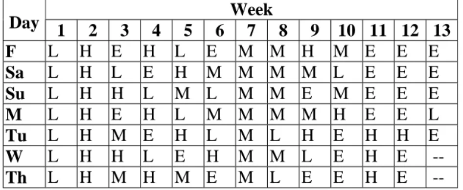
Using these methods, we scheduled periods of ventilation in each of the four control modes: low, medium, high, and economizer mode. The intent to have a schedule of randomized ventilation rates that changed daily during weeks 3 – 6 and 8-10, was met reasonably well. During weeks 1,2, 7, 11 and13, we intended to fix the ventilation rates at the low, medium, high, or economizer setting for one week periods; however, the ventilation-rate control system failed during some periods. The resulting schedule of ventilation control modes is provided in Table 1. The control system resulted in a wide range of ventilation rates; however, these ventilation rates were not sufficiently repeatable to use the control mode as a categorical surrogate for the ventilation rate. Thus, measured ventilation rates and carbon dioxide concentration were used in analyses of the productivity data.
Table 1. Ventilation control schedule. L, M, and H refer to fixed damper positions for low, medium, and high ventilation rates. E refers to control of ventilation rates by the economizer control system. Week Day 1 2 3 4 5 6 7 8 9 10 11 12 13 F L H E H L E M M H M E E E Sa L H L E H M M M M L E E E Su L H H L M L M M E M E E E M L H E H L M M M M H E E L Tu L H M E H L M L H E H H E W L H H L E H M M L E H E -- Th L H M H M E M L E E H E -- Carbon dioxide concentrations
CO2 concentrations were measured in the return airstreams of all AHUs as described above.
Concentrations in return airstreams represent an approximate average of the concentration of CO2 in the associated occupied spaces of the building. The difference between indoor CO2
concentrations and outdoor concentrations (∆CO2) is not easily related to accurate estimates of
rates of outside air supply; however, these ∆CO2 concentrations are measures of the degree of
control of occupant-generated air pollutants via outside air ventilation. Indoor temperatures and humidities
Air temperatures and humidities were measured approximately one meter above floor level throughout the spaces occupied by the study population. The approximate location of each worker (identified only with an agent code number) was provided by the building manager; thus, each worker was associated with nearby measurements of temperature and humidity.
Temperatures were logged every one minute at 25 indoor locations with two types of battery-powered loggers3. Relative humidities were logged every five or 15 minutes at 11 indoor locations using battery-powered relative humidity loggers4.
Collection of worker performance data and associated data
The call center’s automated call distribution (ACD) system monitors several performance-related parameters. Worker performance for each half-hour period is summarized with the “average handle time”(AHT) of all of the calls that ended during that period. The AHT is the average time (averaged over all agents and over the entire half hour) taken for each call from beginning
3Ten Onset Instrument, HOBO-Pro Series Temp Ext (C) loggers with a resolution of 0.02 oC and rated accuracy of ±0.2 oC; and 15 Onset Instrument, StowAway-Temp (C) loggers with a resolution of 0.3 oC and rated accuracy of ±0.3 oC. The calibration of the HOBO-Pro Series temperature loggers was checked by comparison to a NIST-traceable RTD system with 0.02 oC rated accuracy. After to the field study, the calibration of the StowAway-Temp loggers was checked with an ice bath and via a sensor intercomparison.
4
Onset Instrument HOBO Temperature, RH (C) with rated accuracy of ±3% RH or Onset Instrument HOBO-RH (C) with rated accuracy of ± 5% RH. Calibrations were checked using the air space in chambers above salt solutions to produce reference values of humidity.
to end, starting when the call was answered and ending when the agent completely finished all tasks associated with the call and was available to answer another call.
In addition to monitoring the handle time, the call center has a target for the amount of time for which callers are desired to be on hold; for the period of the study, the target time was four minutes for registered nurses, and 1:50 for TSRs. From the point of view of the call center's managers, a waiting time that is "too short" means that too many agents were available to answer calls, while a waiting time that is "too long" means that not enough agents were available or that the agents were working too slowly. Long wait times cause some callers who have been on hold for a long time to spend some time complaining about the wait before getting down to business, leading to longer calls and thus tending to further increase the queue of waiting callers.
Complicating the issue of wait times is that agents can see a large electronic display on the wall, indicating both the number of calls on hold and the longest time that any of the callers have been waiting. The call center managers believe that this display motivates the agents to work faster when the queue gets long, because they don't like talking with irritated callers, and this effect may partially counteract the tendency for callers who have been holding for a long time to take longer to complete their calls.
For each half-hour period, the call center's computer calculates and records a number, called "nets", that summarizes how well the agents were able to meet the demands of the callers. Nets is an estimate of how many extra agents were on hand, compared to the number needed to meet the target wait times, based on the number of calls received and the observed AHT. For periods when the target wait times were exceeded, nets is negative. Nets is used as a variable in the data analyses as described subsequently.
Statistical analyses
Our primary interest was the relationship between ventilation rate and worker performance ---measured, in this case, by AHT. Ventilation rate was expected to influence AHT by at most a few percent, which is less than the variation due to several other sources. In principle, in a very long study using randomized levels of ventilation rate, the other sources of variation would cancel out any effects of changes in ventilation could be examined with a simple categorical analysis. In practice, with only twelve weeks of data, randomization of ventilation would not necessarily be sufficient to ensure that other sources of variation cancel out completely.
Therefore, to estimate effects of ventilation-related variables with useful precision we excluded some data from the analyses and controlled for other sources of variation in AHT using
multivariate regression models.
The number of calls varied greatly throughout the day, as did the number of workers (called “agents”) scheduled to handle them. Carbon dioxide concentrations (and, presumably, other pollutants associated with human bodies) were never high outside the normal workday (7:30 a.m. –6:00 p.m. Monday through Friday). Although excluding data collected from nights and
weekends significantly reduced the amount of data analyzed, the alternative was to rely on regression modeling alone to relate performance during the night-time and weekend, when CO2
concentrations were always low, to performance during the weekday periods with a wide range of carbon dioxide levels. We did not trust such modeling to be free of small sources of bias that
could overwhelm the small expected effects of ventilation rate on worker performance;
consequently, we elected to discard data outside the normal work week (Monday – Friday, 7:30 a.m. – 6:00 p.m.).
The tasks performed by the appointment schedulers (the TSRs) were simpler than those
performed by the registered nurses (RNs). The RNs had some “wrap-up” time associated with most calls, during which they create a computer record of the medical problem and their response to it. For both RNs and TSRs, the time required to handle a particular call was substantially dependent on the caller rather than on the agent, but RNs can have a larger influence on their own work rate. Therefore, we concentrated most of our efforts on analyzing the RN data and all of the results provided below are for RNs.
Data from Labor Day (a Monday) and the following day were clearly anomalous in the number of calls, although this is not reflected in unusual values of AHT: many fewer people called on Labor Day than on a typical Monday, and more people than usual called on the following day. We excluded data from Labor Day and the following day from the analyses.
Data from two additional days were excluded. Substantial changes to the computer software used by the agents were made just before the start of the study, so we excluded what would otherwise have been the first day of the study (a Friday) to try to avoid data affected by the learning period. Further software changes were made on day 58 of the study (a Saturday), and these changes apparently slightly affected AHT (by increasing it) until workers became
accustomed to the changes. For this reason, we excluded day 60 (a Monday).
Except where specified, all results below are based only on RN data from 7:30 a.m.- 6:00 p.m. Monday through Friday, excluding Labor Day and the following day, and excluding day 1 and day 60.
Linear regression was our main tool for analyzing the data: we regressed AHT or log(AHT) on explanatory variables that are expected to be relevant. Although we performed analyses using both AHT and log(AHT), we favor the log transformation for two reasons: the resulting residuals have a distribution that is closer to normal; and we anticipate that changes in environmental factors (or in other confounding factors) that reduce or increase work rate should increase or decrease AHT by a relative rather than an absolute amount. In this paper, we report results only for analyses based on log(AHT).
We have no direct measurements of noise, call content, caller cooperation, worker motivation, and other factors that are expected to directly influence agent performance, but we do have explanatory variables that serve as proxies for these parameters:
1. Noise and level of activity are related to the number of agents working at a given time, so we included the number of agents as one of our explanatory variables.
2. Callers’ cooperation and workers’ motivation were both expected to be related to queue length, so we included the "nets" variable.
3. Call content was expected to vary with queue length (due to caller abandonment), and also with time of week, so we included time-of-week indicator variables in the regression.
4. Indoor air pollution levels were not directly measured with useful frequency, but indoor and outdoor carbon dioxide were measured every half hour. CO2 never reached levels at which it
would directly affect performance. However, the difference between the indoor and outdoor concentration (∆CO2) concentration is a proxy for ventilation per agent. The difference between
indoor and outdoor CO2 concentrations, ∆CO2, should be correlated with the indoor
concentration of any pollutant emitted indoors at a rate that is approximately proportional to the number of people in the building. Examples of such pollutants are body odors, perfumes, dust stirred up by activity, and emissions from equipment used by occupants such as computers and copy machines.
We cannot expect to perfectly adjust for all of the actual sources of variation in AHT. Instead, the goal was to adjust for systematic variation that could interfere with obtaining accurate estimates of the effects of ventilation-related variables.
As illustrated subsequently, AHT varied systematically throughout the day and throughout the week. To control for this systematic variation, we created time-of-week indicator variables for each half-hour period. These time-of-week indicator variables alone accounted for about 35% of the variation in log(AHT).
We performed a variety of regressions on log(AHT), using different combinations of explanatory variables chosen from the following:
1. time-of-week indicator variables;
2. building-average temperature (Celsius) – 23 oC;
3. (building-average temperature-23 oC)^2 was included as a variable to account for the possibility of a non-linear relationship between temperature and performance, e.g., a temperature associated with maximum performance;
4. building-average relative humidity;
5. number of agents on duty---we have data on RNs and TSRs separately. Using the RN occupancy number alone provided a slightly better fit to the RN data.;
6. normalized “nets” (piecewise linear), normalized to the number of workers on duty; for example, if 30 agents were working, and nets equaled 3, normalized nets was 0.1, since there was a 10% surplus of agents;
7. indoor-outdoor carbon dioxide concentration difference (linear or categorical, or piecewise linear).
The piecewise-linear model for “nets” divided the parameter into bins, and assumed that within each bin the parameter had a linear influence on log(AHT), but we allowed the different bins to have different slopes and intercepts.
For each model, we first performed an ordinary regression of log(AHT) on the explanatory variables, weighting each data point by the number of calls received during the half hour. Eighty percent of the half-hour periods in our analysis included between 130 and 260 calls, so the weights were not highly variable, nor were they very influential. After fitting the model, we calculated the serial correlation of the residuals, as a function of time lag. In every model the lagged serial correlation was moderately high (greater than 0.2) for lags of a few hours, but dropped to near zero over several hours. The temporal correlation reduced the statistical power
of the analysis: effectively, if observations were highly correlated, then each observation added less independent information. We used the observed serial correlation (or, rather, the observed lagged covariance) to estimate the variance-covariance matrix of the residuals, assuming the covariance to be identically zero for time lags exceeding six hours. Following a standard approach for regression in which the residuals have an off-diagonal variance-covariance matrix (e.g. see Box et al., p.363 or Gelman et al., p. 257), we then performed a linear regression that used the same explanatory variables but adjusted for the temporal correlation of the residuals. Compared to the conventional regression, in which observations are assumed to be independent, the coefficient estimates changed by a small amount and width of the error bars increased slightly.
Results
Ventilation rates and ∆CO2 concentrations
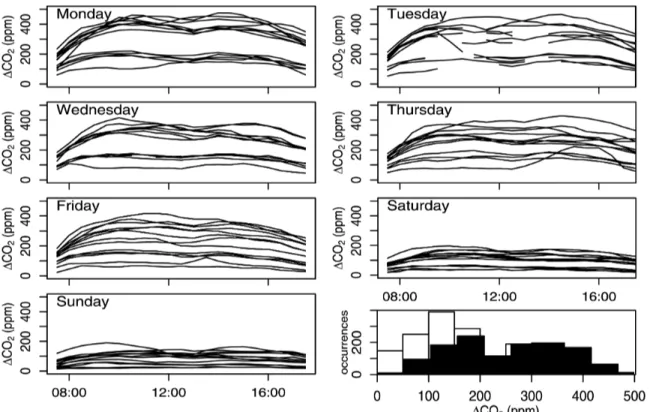
Figure 1 shows the ∆CO2 concentration versus time, separately for each day of the week, with all
weeks superimposed. Only data from 7:30 a.m. to 6:00 p.m. are shown. The lower right plot in the figure shows histograms of the carbon dioxide concentration difference for all of the days (upper line in each bin), and also for just Monday through Friday (lower line in each bin). As the histogram shows, ∆CO2 on weekends was never above 200 ppm, and ∆CO2 concentrations on
weekdays were rarely below 100 ppm.
Figure 1. Time trends and histogram for the differences between indoor and outdoor carbon dioxide concentrations. In time trends, each line represents data from a workweek. In the histogram, the upper line in each bin reflects from 7:30 a.m. to 6:00 p.m. of all days while the lower line (shaded section) represents data from the same periods of Monday through Friday.
Figure 2 shows ∆CO2 versus ventilation rate (flow rate of outside air supply), displaying all of
the data for the entire study (not just the normal work week). Superimposed is a line showing the results of a local robust regression using the lowess method (Cleveland, 1979; with a smoother span of 1/5, and 3 iterations). ∆CO2 values tend to cluster into three wide clumps,
corresponding to low, medium, and high damper settings, with “economizer” settings also tending to lead to fairly low or very low values of ∆CO2.
Figure 2. Average handle times (AHTs) of RNs. In the time trends, each line represents data from a workweek.
∆CO2 varies with both ventilation rate and the number of people in the building; in steady state,
the concentration would be nearly proportional to the number of people, and inversely
proportional to the ventilation rate. Thus a given ventilation rate can correspond to a wide range of carbon dioxide concentrations (or other pollutants associated with the presence of people). Average Handle Times
Figure 3 shows AHT versus time of day, separately for each day of the week, showing only the data from 7:30 a.m.- 6:00 p.m., and overlaying data from all 12 weeks. As the plot shows, the AHT varies throughout the day, and from day today throughout the week. The variation may ultimately be due to several causes, including variation in call content (the things people want to
talk about early in the morning differ from those later in the day), and in worker alertness and fatigue. During the normal workday, 7:30 a.m.- 6:00 p.m. Monday through Friday the AHT ranges from about 500 seconds in the morning to about 540 seconds in the evening, as well as varying slightly from day to day.
Figure 3. Indoor minus outdoor carbon dioxide concentrations plotted versus ventilation rates.
Temperatures and humidities
The building’s climate control held the building-average temperature within a very narrow range during working hours. Fifty percent of the half-hourly work-day temperatures were between 23.1
o
C and 23.3 oC, and ninety percent were between 22.9 oC and 23.5 oC. Building average humidity was also rather constant, almost never straying outside the range 46% to 47%. The very narrow observed ranges of these parameters yielded low statistical power to estimate coefficients of these variables. Unsurprisingly, then, the regression coefficients associated with temperature, (temperature – 23 oC)^2, and relative humidity, are all very small compared to their uncertainties.
For modeling worker performance and environmental factors, discussed below, we fit models both with and without temperature and humidity data; including these variables had very little effect on the estimates for the main parameters of interest. The results presented are from models with temperature and humidity included as variables.
Association of worker performance with environmental factors
We fit several dozen regression models, using different definitions for the bin boundaries for number of calls, normalized nets, and ∆CO2, and using different subsets of the data. Measures of
model fit were very similar for all models that included the full set of explanatory variables, whatever the details of the model.
In every model that we tried, including Models A-C discussed below, the “nets” variables were found to be highly influential. For example, when nets was very negative---that is, when there were many more calls than the agents were able to handle---log(AHT) was elevated by more than 7% compared to the same day and time of day in different weeks. This effect is
substantially larger than any expected effect of ventilation, so failure to accurately model the variation of log(AHT) with “nets” could potentially overshadow a ventilation effect. The five-category piecewise-linear relationship between log(AHT) and “nets” that we used in the models allows a more complicated relationship between nets and AHT than would an assumed linear or quadratic relationship across the whole range of “nets” values.
We also included half-hour lagged “nets” in the regressions. Lagged “nets” is the value of “nets” in the previous half-hour. This variable, which was found to be influential, may be important because some calls that terminated in a given half-hour were started in the previous one, and because lagged nets may help predict agent fatigue. Additionally, the mix of calls in a given half-hour period is affected by the wait times from the previous periods: some callers who abandoned calls in the previous period will call back. Although we also examined non-linear relationships between lagged “nets” and log(AHT), these models provided no advantage over linear models for this variable. In the models discussed below, we assumed log(AHT) to vary linearly with lagged “nets.”
We now discuss three specific models for log(AHT) in some detail. Each of these models includes: the time-of-week indicator variables; temperature – 23 oC and (temperature – 23 oC)^2; number of agents on duty; five piecewise-linear “normalized nets” categories; and lagged “nets”, allowing linear variation of log(AHT) with the “nets” value of one half hour previous. The three models differ only in their handling of ∆CO2. Model A includes no ∆CO2 variable. Model B
includes three ∆CO2 categorical variables, indicating whether ∆CO2 for each half hour was:
0-150 ppm, 0-150-300 ppm, or over 300 ppm. In Model C, the two lower ∆CO2 categories within
Model B have been split, thus, Model C has five ∆CO2 categorical variables: 0-75 ppm, 75-150
ppm, 150-225 ppm, 225-300 ppm, or over 300 ppm. Table 2 identifies the variables used in each model and provides some of the regression coefficients and associated uncertainties.
Table 2: Regression coefficient estimates and standard errors for three statistical models of log(AHT) on the listed set of explanatory variables. Coefficient estimates for the 105 time-of-week effects, five “nets” categories, and five “nets” slopes are not shown, but are similar for all three models.
Coefficient estimate [units] Model A Model B Model C
<Time of week> [log(AHT)]
Included in model Included in model Included in model < five “nets” categories>
[log(AHT)]
Included in model Included in model Included in model < five “nets”slopes>
[log(AHT) / nets]
Included in model Included in model Included in model Lagged “nets” [log(AHT) / nets] 0.048 +/- 0.015 0.053 +/- 0.015 0.054 +/- 0.015 (temp – 23 oC) [log(AHT) / degree C] -0.24 +/- 0.45 -0.23 +/- 0.44 -0.13 +/- 0.43 (temp – 23 oC)^2 [log(AHT) / (degree C)^2] 0.007 +/- 0.027 0.006 +/- 0.03 0.004 +/- 0.029 Relative Humidity [log(AHT) / % ] 0.11 +/- 0.22 0.11+/- 0.22 0.06 +/- 0.22 Agents on duty [log(AHT) / agent] 0.0016 +/- 0.0004 0.0017 +/- 0.0004 0.0017 +/- 0.0004 0 < ∆CO2 < 75 [log(AHT)] Not in model 0.00 +/- 0.00 0.00 +/- 0.00 75 < ∆CO2 < 150 [log(AHT)]
Not in model Not in model 0.036 +/- 0.010
150 < ∆CO2 < 225
[log(AHT)]
Not in model -0.002 +/- 0.004 0.031 +/- 0.010 225 < ∆CO2 < 300
[log(AHT)]
Not in model Not in model 0.027 +/- 0.010
300 < ∆CO2
[log(AHT)]
Not in model -0.009 +/- 0.006 0.022 +/- 0.010
[log(AHT)]Residual standard error 0.0446 0.0445 0.0442
Figure 4 shows the residuals from Model A (which did not include ∆CO2), plotted versus ∆CO2.
A lowess local regression fit is shown as a solid line (we used a smoother span of 1/5, and 3 iterations). Only for low ∆CO2 values is there any evidence that the residuals might vary with ∆CO2; the model tends to predict longer handle times than were actually observed for very low ∆CO2 concentrations. The right-hand portion of Fig. 4 shows a histogram of the residuals, with a
Normal distribution (mean 0, standard deviation 0.0448) superimposed. The distribution of residuals is very close to Normal, as we assume when we perform least-squares regressions.
Figure 4. Residuals from regression model A, which does not include a carbon dioxide variable, versus indoor minus outdoor carbon dioxide concentration.
Figure 5 shows the estimated model coefficients associated with each ∆CO2 bin, for Models B
(lower plot) and C (upper plot). For each bin, the horizontal bar shows the range of ∆CO2
spanned by the bin, and the vertical error bar covers plus or minus one standard error. In each case, the lowest bin is defined to have no effect, a coefficient of 0.00.
Figure 5. Model coefficients for bins of ∆CO2 concentration, indicating the effect of ∆CO2 on
log(AHT) with the lowest ∆CO2 bin used as the reference. The lower and upper plots are results
of Model B and Model C, respectively. Horizontal bars indicate ∆CO2 bin boundaries and
In the model with only three ∆CO2 bins (Model B) there is no evidence that lower ∆CO2 is
associated with lower (faster) AHT---indeed, the relationship points the other direction: the estimate for the high-∆CO2 bin is about 1% faster than that for the lowest bin (an effect of -0.009
on log(AHT) corresponds to a factor of exp(-0.009)=0.991 on AHT, which is very close to a 1% speed-up). However, this estimate is not very precise, with an uncertainty (one standard error) of approximately ± 0.6 percentage points.
In contrast, the results from Model C suggest that very low ∆CO2 concentrations are associated
with lower AHT (faster work) than are higher concentrations. All of the estimated coefficients for ∆CO2 concentrations over 75 ppm are around 0.025 to 0.035, corresponding to handle times
that are 2.5% to 3.5% slower than at the lowest ∆CO2. Moreover, these effects are all highly
statistically significant (p < 0.05 for all bin coefficients). However, as we discuss below, we think the statistical uncertainties are understated and that the relationship between AHT and ∆CO2 is far from conclusive.
Overall, as Figure 5 shows, neither the Model B nor Model C results show evidence that handle time increases with ∆CO2 over most of its range. A dependence of log(AHT) on ∆CO2 is
apparent only for ∆CO2 concentrations below about 150 ppm: log(AHT) is somewhat lower for ∆CO2 concentrations in the 0-75 ppm range than in the 75-150 ppm range, after adjusting for all
of the other explanatory variables. When the 0-150 ppm ∆CO2 category is split into two
categories, as in Model C, the 0-75 ∆CO2 category has the lowest (fastest) values of log(AHT),
after adjusting for the other explanatory variables. But when the ∆CO2 data from 0-150 ppm are
combined into a single bin, as in Model B, the overall average AHT in this bin is about the same as in the other bins.
In another model, we treated ∆CO2 as a continuous variable throughout the entire concentration
range and found no statistically significant or strong relationship between ∆CO2 and AHT.
These findings were essentially unchanged, when data collected after day 57 were excluded from the analyses in order to eliminate any possible effects of the change in software on day 58. The analyses based on ∆CO2, which is a proxy for ventilation per person, assume that effects on
AHT would be caused by pollutants with indoor concentrations approximately proportional to the number of people. This covers a wide range of pollutants, including body odors, dust stirred up by activities, emissions from computers and similar devices, detergent residues on clothes, fibers and dust from clothes, and so on. However, the building itself can also be a source of pollutants, independent of the number of people in it: walls or carpeting may emit volatile organic compounds, for example. If the building is the source of pollutants that affect performance, then it is total ventilation rate, not ventilation per person, that should predict variation in AHT. We investigated this possibility by fitting Models like A-C, but using ventilation rate categories rather than ∆CO2 categories. There is no evidence for a dependency
of AHT on ventilation rate; in fact, even for the highest values of ventilation rate there is no evidence for reduced handle time compared to lower ventilation rate values. To the extent that there is an apparent ventilation-related effect in this study, it is due to ventilation rate per person (as indicated by ∆CO2) rather than ventilation per unit indoor air volume.
Discussion
Considering that all of the workers in the study received at least the code-minimum ventilation, any performance differences associated with ventilation would be expected to be only a few percent at most. It is very hard to design an experiment to quantify such small performance differences in the real world. The analysis of the call center experiment that is described in this paper has inadequate statistical power to find effects smaller than about 2%.
Several characteristics of the call center (or, indeed, of almost any potential study environment) differ from the environments of controlled small-scale experiments. For example, new workers are hired and become part of the work place, while others quit and drop out. Presumably, the new workers are slower than experienced workers, because they haven’t learned all the tricks of the trade; or perhaps they are faster, because they are under increased scrutiny or because the novelty keeps them more alert. Changes to software may have effects that are virtually
impossible to estimate; for instance, changes may first slow the workers down as they learn the new software, but then speed them up in the long run if the software allows them to work more efficiently. The mix of call types, and thus the average handle time, may change subtly over long periods, perhaps, for this medically-related call center, depending on the types of illnesses that become more or less common over the study period. Over a very long study period these effects will cancel out, if the ventilation parameters are randomized, but over a short period any chance correlation between ventilation-related parameters and the other effects can eliminate the ability to determine the effects related to ventilation.
In the present study, in the M-F, standard workday data there were only forty half-hour periods (out of 1051) in which the ∆CO2 concentration was below 75 ppm. Nineteen of these periods
occurred on a single day (the 78th day of the study, a Friday), and all of the rest occurred during the following week, very close to the end of the 88-day study. The entire apparent speed-up in AHT indicated by Model C, for the below-75 ppm bin relative to the others, is based on data from only six different days, and 65% of those data are from two consecutive Fridays. In our analysis, when calculating standard errors (and p-values) we took into account the intra-day correlation in residuals in order, but not the correlation over longer periods. Throughout the study, day-to-day and week-to-week correlation in residuals was usually very low; however, there are some periods in which correlation is evident across several days. One example is days 58-60, discussed previously, when new software led to increased AHT (compared to what the models predict) for several consecutive days. Although investigation of the data and residuals reveals nothing suspicious about the days during which the ∆CO2 concentrations were very low,
the possibility of an unknown effect that led to decreased AHT during that period cannot be ruled out, and is not accounted for in the model. Consequently; in spite of the low p-values, we do not consider the results of Model C to conclusively indicate a faster work-rate when ∆CO2 was very low and ventilation per worker was very high. If the very high values of ventilation had occurred on 6 days spread throughout the study period, and the same analyses resulted, we would have confidence that the observed effect is really due to ventilation; in the present case, though, we are simply not sure.
One limitation in these analyses is a consequence of the incomplete separation of time of day from ∆CO2. As time of day increases, ∆CO2 generally increases (and then decreases late in the
workday when occupancy is reduced); therefore; controlling for time of day via the regression models could have partially obscured a relationship of ∆CO2 with worker speed. Including nets
in the regression models may also have partially obscured a relationship of ∆CO2 with worker
speed, because a decrease in work speed caused by higher ∆CO2 would result in a decrease in
nets.
We have used ∆CO2 as a surrogate of ventilation rate per person, recognizing that previous
studies have demonstrated the difficulty of accurately computing the ventilation rate per person from CO2 measurements. The errors result primarily from variable occupancy, variable outside
air supply rates, failure to measure outdoor CO2 concentrations, and inaccurate CO2
measurements. In this study, outdoor CO2 concentrations were measured and all measurements
were made with research-grade, frequently-calibrated instruments. In addition, outside air supply rates were relatively stable, except in the economizer control mode. Despite these efforts to reduce errors, we do not claim that ∆CO2 data can be precisely converted to ventilation rates
per person. Nevertheless, it is clear that the categories of ∆CO2 used in our analyses represent
different average ventilation rates per person.
More sophisticated analyses should allow us to reduce uncertainties somewhat, beyond those presented in this paper. For example, in addition to the time-resolved data discussed here, we also have data on the performance of each agent, averaged over each of their work shifts during the study period. Since some agents work faster than others, day-to-day variation in which agents are at work is a source of variation in AHT. By estimating average work rates for each agent we should be able to partially adjust for this effect, thus slightly reducing the unexplained variation in AHT.
Conclusions
If we exclude periods of very high ventilation rates per occupant (indicated by very low ∆CO2)
experienced during the study, we can rule out effects on AHT that are greater than about 2%. There is no evidence of any effect at all, although the present analysis does not have sufficient statistical power to eliminate the chance of effects in the 1% range; such effects, if they occur, would still be of practical importance.
There is some evidence that very high ventilation rates per occupant (very low ∆CO2) may lead
to lower AHT (faster work rates), but the possibility of an unknown confounding variable makes this result less than conclusive in spite of high statistical significance (p < 0.05). The statistical model from which the p-values were derived assumes that no temporal correlation in the
residuals lasts more than one work day. A “one-time-only” event that lowered AHT slightly (on average) for a week cannot be ruled out, and could be the real cause of the apparent ventilation effect.
The results of the present analysis may not apply to other buildings, or even to other call centers. For instance, it may be that in this building there are no strong indoor sources of pollutants that
influence performance, but that in other buildings such sources exist. If that is the case, then ventilation may have larger effects in those other buildings.
Acknowledgments
This work was supported by the Assistant Secretary for Energy Efficiency and Renewable Energy, Office of Building Technology, State, and Community Programs, Office of Building Research and Standards of the U.S. Department of Energy (DOE) under contract No. DE-AC03-76SF00098 and by the Center for the Built Environment at U.C. Berkeley. The authors thank Michael Sohn and Michael Apte for their reviews of a draft of this paper.
References
Apte, M.G. and Daisey J.M. (1999) VOCs and "Sick Building Syndrome": Application of a new statistical approach for SBS research to U.S. EPA BASE Study data. In Proceedings of Indoor Air’99, vol 1, pp. 117-122, Construction Research Communications, Ltd., London.
Box GEP, Jenkins GM, Reinsel G, 1994. Time Series Analysis, New Jersey: Prentice Hall.
Cleveland, WS. 1979. Robust locally weighted regression and smoothing scatterplots. J. Amer. Statist. Assoc.
74:829-836.
Gelman A, Carlin JB, Stern HS, and Rubin DB, 1995. Bayesian Data Analysis. New York: Chapman and Hall. Kroner WM, Stark-Martin JA. (1992). Environmentally responsive workstations and office worker productivity. Ed. H Levin, Proc. Indoor Environment and Productivity, June 23-26, Baltimore, MD, ASHRAE, Atlanta. Lagercrantz L, Wistrand M, Willen U, Wargocki P, Witterseh T, Sundell J (2000) Negative impact of air pollution on productivity: previous Danish findings repeated in a new Swedish test room. Proceedings of Healthy Buildings 2000, vol. 1., pp 653-658. August 6-10, Helsinki. SIY Indoor Air Information, Oy, Helsinki.
Mendell MJ. 1993. Non-specific symptoms in office workers: a review and summary of the epidemiologic literature. Indoor Air 3: 227-236.
Menzies D, Bourbeau J. 1997. Building-related illness. New England Journal of Medicine 337(21): 1524-1531. Myhrvold AN, Olsen E, Lauridsen O. 1996. Indoor environment in schools – pupils health and performance in regard to CO2 concentrations. Proc. Indoor Air 1996, The 7th International Conference on Indoor Air Quality and Climate. 4: 369-374. SEEC Ishibashi Inc., Japan.
Myhrvold AN, Olsen E. 1997. Pupils health and performance due to renovation of schools. Proc. Healthy Buildings / IAQ 1997. 1: 81-86. Healthy Buildings / IAQ 1997. Washington, DC.
NEMA. 1989. Lighting and human performance: a review. Washington, D.C. National Electrical
Nunes F, Menzies R, Tamblyn RM, Boehm E, Letz R. 1993. The effect of varying level of outside air supply on neurobehavioral performance function during a study of sick building syndrome. Proc. Indoor Air 1993, The 6th International Conference on Indoor Air Quality and Climate. 1: 53-58. Indoor Air 1993, Helsinki.
Seppanen OA, Fisk WJ, Mendell MJ. 1999. Association of ventilation rates and CO2-concentrations with health and
Sundell J. 1994. On the association between building ventilation characteristics, some indoor environmental exposures, some allergic manifestations, and subjective symptom reports. Indoor Air: Supplement 2/94.
Ten Brinke, J.; Selvin, S.; Hodgson, A.T.; Fisk, W.J.; Mendell, M.J.; Koshland, C.P.; and Daisey, J.M. (1998) “Development of new VOC exposure metrics and their relationship to sick building syndrome symptoms”, Indoor Air 8(3): 140-152.
U.S. Department of Commerce, Bureau of the Census. Table 645, Statistical Abstract of the United States (117th ed.), 1997.
Wargocki P. 1998. Human perception, productivity, and symptoms related to indoor air quality. Ph.D. Thesis, ET-Ph.D. 98-03, Centre for Indoor Environment and Energy, Technical University of Denmark, 244 pp.
Wargocki P, Wyon DP, Sundell J, Clausen G, and Fanger PO (2000a) The effects of outdoor air supply rate in an office on perceived air quality, sick building syndrome (SBS) symptoms, and productivity. Indoor Air 10(4): 222-236
Wargocki P, Wyon DP, and Fanger PO (2000b) Productivity is affected by air quality in offices. Proceeding of Healthy Buildings 2000, vol. 1, pp 635-640. August 6-10, Helsinki. SIY Indoor Air Information, Oy, Helsinki. Wargocki P, Wyon DP, and Fanger PO (2000c) Pollution source control and ventilation improve health, comfort, and productivity. International Centre for Indoor Environment and Energy, Danish Technical University. Submitted for presentation at Cold Climate HVAC 2000, November 1-3, 2000, Sapporo, Japan.
Woods JE. 1989. Cost avoidance and productivity in owning and operating buildings. Occupational Medicine 4 (4): 753-770.
Wyon DP, Andersen IB, Lundqvist GR. 1979. The effects of moderate heat stress on mental performance.
Scandinavian. J. Work Environment and Health. 5: 352-361.
Wyon DP. 1993. Healthy buildings and their impact on productivity. Proc. Indoor Air'93, the 6th International Conference on Indoor Air Quality and Climate. 6: 3-13. Helsinki. Indoor Air 93.
Wyon DP. 1996a. Indoor environmental effects on productivity. Proc. IAQ’96 “Paths to Better Building Environments”. pp 5-15, ASHRAE, Atlanta.
Wyon DP. 1996b. Individual microclimate control: required range, probable benefits, and current feasibility. Proc. of Indoor Air 96. 1:1067-1072. Tokyo. Institute of Public Health.