Tuomas Matikka
The Elasticity of Taxable Income:
Evidence from Changes in
Municipal Income Tax Rates in
Finland
VATT WORKING PAPERS
69
The Elasticity of Taxable Income:
Evidence from Changes in
Municipal Income Tax Rates in Finland
Tuomas Matikka
Tuomas Matikka, VATT Institute for Economic Research (Helsinki, Finland),
tuomas.matikka@vatt.fi, Tel +358295519461
ISBN 978-952-274-165-3 (PDF)
ISSN 1798-0291 (PDF)
Valtion taloudellinen tutkimuskeskus
VATT Institute for Economic Research
Arkadiankatu 7, 00100 Helsinki, Finland
Helsinki, December 2015
The Elasticity of Taxable Income: Evidence from Changes
in Municipal Income Tax Rates in Finland
VATT Institute for Economic Research
VATT Working Papers 69/2015
Tuomas Matikka
Abstract
The elasticity of taxable income (ETI) is a key parameter in income tax analysis
both in terms of efficiency and tax revenue. This paper uses Finnish panel data to
analyze ETI. I use changes in flat municipal income tax rates as an instrument for
overall changes in marginal tax rates. This instrument is not a function of
individual income, which is the basis for an exogenous instrument. In general,
instruments used in previous studies do not have this feature. My preferred
estimate for the average ETI is 0.16. The preferred specification includes
extensive regional and individual controlling.
Earlier version of this paper was published in February 2014 ("Taxable income
elasticity and the anatomy of behavioral response: Evidence from Finland"
Government Institute for Economic Research (VATT) Working Papers 55).
Key words:
elasticity of taxable income, income taxation
JEL classes:
H21, H24, J22
Tiivistelmä
Tässä tutkimuksessa tarkastellaan verotettavan tulon joustoa (elasticity of taxable
income) Suomessa vuosina 1995–2007. Verotettavan tulon jousto on keskeinen
tekijä verotuksen taloudellisen tehokkuuden ja veronmuutosten vaikutusten
arvioinnissa. Verotettavan tulon jousto mittaa sitä, kuinka paljon tuloverotuksen
veropohja eli verotettava tulo keskimäärin muuttuu, kun yhdestä lisäeurosta
käteen jäävä osuus (1-rajaveroaste) muuttuu yhden prosentin. Korkeampi
rajaveroaste voi esimerkiksi vähentää tehtyjä työtunteja sekä lisätä
verosuunnittelua ja verovähennysten käyttöä. Verotettavan tulon jousto huomioi
eri kanavat joilla tuloverotukseen voidaan reagoida.
Tutkimuksessa hyödynnetään kunnallisveroprosenteissa tapahtuneita muutoksia
veroastevaihtelun lähteenä. Kunnallisverotus tarjoaa hyvän vertailuasetelman,
sillä kunnallisveroprosentit ovat muuttuneet eri tavalla eri puolella Suomea eri
vuosina. Lisäksi kunnallisveroprosentti ei riipu henkilön tuloista, joten
kunnallisveroprosentin muutokset aiheuttavat muutoksia rajaveroasteissa kaikissa
tuloluokissa.
Tulosten perusteella verotettavan tulon jousto on Suomessa keskimäärin noin
0,15. Tulosta voidaan tulkita siten, että tuloverotuksen kiristäminen
(keventäminen) pienentää (kasvattaa) verotettavaa tuloa tilastollisesti
merkitsevällä tavalla, mutta tuloverotuksen aiheuttama hyvinvointitappio on
kokonaisuudessaan maltillinen.
Tutkimuksen aikaisempi versio on julkaistu VATT:n Working Papers-sarjassa
helmikuussa 2014 ("Taxable income elasticity and the anatomy of behavioral
response: Evidence from Finland" Government Institute for Economic Research
(VATT) Working Papers 55).
Asiasanat:
Tuloverotus, verotettavan tulon jousto, hyvinvointitappio
Contents
1 Introduction 1
2 Conceptual framework 4
3 Finnish income tax system and recent changes in tax rates 6
3.1 Institutional setting . . . 6
3.2 Recent changes in income tax rates . . . 7
4 Data and identification 9 4.1 Data . . . 9
4.2 Individual tax rate variation . . . 10
4.3 Net-of-tax rate instrument . . . 13
4.4 Descriptive statistics . . . 15
4.5 Empirical specification . . . 17
5 Results 19 5.1 Main results . . . 19
5.2 Alternative specifications and robustness checks . . . 21
5.2.1 Subcomponents of taxable income . . . 21
5.2.2 Robustness checks . . . 22
1
Introduction
The elasticity of taxable income (ETI) with respect to the net-of-tax rate (one minus the marginal income tax rate) is a key tax policy parameter and an important element in the efficiency analysis of income taxation. The practical significance of ETI is straightforward: it measures how a one percent change in the net-of-tax rate affects taxable income. Intuitively, the more elastic taxable income is, the larger the behavioral response to a tax reform will be, in terms of a change in the tax base. Therefore, good knowledge of ETI is essential when deciding on national tax reforms.
Furthermore, ETI measures the overall marginal excess burden of income taxation (Feldstein (1995, 1999), Saez, Slemrod and Giertz (2012)). In addition to labor supply responses, ETI covers other decisions in response to income taxation, such as effort and productivity, deduction behavior, tax evasion and tax avoidance. All behavioral responses reflect the inefficiency of the income tax, and thus different behavioral margins are all important when considering the overall efficiency of the income tax system.
This paper studies ETI using Finnish register data from 1995-2007. I use changes in flat municipal income tax rates as instruments for the changes in overall net-of-tax rates. This instrument is not based on individual income, which provides the basis for an exogenous instrument. In contrast, pre-vious ETI studies typically use instruments that are a function of taxable income. Recent literature highlights that these so-called predicted net-of-tax rate instruments are not necessarily exogenous (Weber (2014), Blomquist and Selin (2010)). This paper proposes an alternative strategy of utilizing institutional features of the tax system to derive an instrument for individual tax rate changes. To my knowledge, this paper is the first to use this type of an instrument to estimate ETI.
In general, variation in tax rates and the endogeneity of the net-of-tax rate variable are the main issues to focus on when estimating ETI using panel data. Identification requires variation in income tax rates that is different for individuals with otherwise similar income trends. Also, due to the progressive income tax rate schedule, a valid instrument for the net-of-tax rate is necessary in order to derive a consistent elasticity estimator. In this study I use variation in municipal-level income tax rates for both purposes.
Finnish municipal income taxation has appealing features from the point of view of empirical ETI analysis. First, the municipal income tax rate is flat, which means that it is independent of individual income level. This is the basis for using changes in municipal tax rates as an instrument for changes in individual net-of-tax rates. Second, differential tax rate variation caused by municipal tax rate
changes covers the entire income distribution. This improves the identification of the average ETI while avoiding some of the typical difficulties in ETI estimation, such as non-tax-related changes in the shape of the income distribution and the mean reversion of income. Third, there is very limited tax rate variation available for individuals at different income levels in Finland. This indicates that changes in municipal tax rates provide the main source of identifying tax rate variation to estimate the average ETI in Finland.
However, even though municipal tax rate changes do not depend on individual income, changes in municipal income tax rates are not randomly assigned to individuals. Municipalities might change their tax rates based on, for example, previous trends in average taxable income in their jurisdiction, which might affect the validity of the instrument. In the paper I provide compelling graphical evidence showing that this type of policy endogeneity is not driving the results. Second, I include different combinations of year and regional fixed effects and municipal-level characteristics (e.g. unemployment and employment rates, municipal debt per capita etc.) in the estimable equation in order to take into account potential regional differences in income trends.
My preferred average ETI estimate is 0.16. The preferred empirical specification includes extensive regional and individual controlling. In addition, as in many earlier studies, the average ETI is slightly larger for women than for men. Also, I find that ETI is somewhat larger for low-income individuals compared to middle and high-income individuals.
In addition, I characterize the structure of the overall response by estimating the elasticity of various subcomponents of ETI, such as labor supply and tax deductions. The analysis of the subcomponents of ETI is useful when designing the income tax system, especially in the light of minimizing the excess burden. Also, it gives information on the economic nature of the response. The results give tentative evidence that both work effort (wage rates) and labor supply (working hours) are not responsive to tax rate changes. However, more irregular components, such as fringe benefits and tax deductions, appear to be more responsive.
The empirical ETI literature has grown substantially following the pioneering studies by Feldstein (1995, 1999). Feldstein (1995) uses panel data to analyze behavioral responses to the 1986 income tax reform in the US. He estimates ETI to be large, ranging from 1-3, depending on the specification used. Many following studies focus on improving the elasticity estimation by paying more attention to the net-of-tax rate instrument and non-tax-related changes in the income distribution. Along with these modifications, ETI estimates decreased markedly compared to those in Feldstein (1995). A
wide range of studies report elasticity estimates ranging from 0 to 0.6. For example, the widely cited Gruber and Saez (2002) study reports the ETI of 0.2 for middle-income earners and 0.6 for high-income earners in the US. An extensive review of earlier empirical results from the US is presented in a recent survey by Saez, Slemrod and Giertz (2012).
More recent papers further study the reliability and consistency of the estimation by utilizing differ-ent tax reforms and differdiffer-ent net-of-tax rate instrumdiffer-ents. This literature underlines that differdiffer-ent tax reforms and more consistent estimation strategies yield different estimates than the seminal con-tribution of Gruber and Saez (2002). In particular, it has been shown that the widely-used predicted net-of-tax rate instruments are not consistent due to potential endogeneity problems. For example, Weber (2014) shows that when using a more robust instrumentation strategy, the ETI estimates are approximately twice as large compared to Gruber and Saez (2002).
A majority of earlier empirical studies estimate ETI using US data sets, while studies concerning European countries and other regions are less common. In particular, there are no earlier Finnish ETI studies available to this day, and thus this paper is the first to comprehensively analyze ETI in Finland. Nevertheless, Pirttilä and Uusitalo (2005) approximate ETI in Finland. Their results suggest that average ETI is around 0.3.
Other Nordic countries (Sweden, Norway, Denmark) provide the closest comparison group to Fin-land in terms of the similarity of the tax system and the overall institutional and cultural framework. Kleven and Schultz (2014) use extensive panel data and many tax reforms to analyze ETI in Den-mark. In general, they obtain a modest average ETI estimate of 0.12. Also, Chetty et al. (2011) report small elasticity estimates using Danish data. Blomquist and Selin (2010) estimate ETI of around 0.20 for males and 1 for females in Sweden. For Norway, Aarbu and Thoresen (2001) find only small responses to tax rate changes. They report that ETI is not significantly different from zero. In a more recent paper, Thoresen and Vattø (2013) report elasticities below 0.1 for Norway. Finally, in addition to previous ETI analysis, this paper relates to other studies that exploit regional within-country variation in tax rates to identify individual-level elasticities. For example, a recent study utilizes changes in municipal-level corporate tax rates to analyze the effect of the corporate tax rate on wages in Germany (Fuest, Peichl and Siegloch (2014)).
The rest of the paper is organized as follows: Section 2 presents the conceptual framework. Section 3 describes the Finnish income tax system and recent changes in income tax rates. Section 4 introduces the data and discusses identification issues. Section 5 presents the results, and Section 6 concludes.
2
Conceptual framework
The basic idea of the taxable income model is that an individual receives positive utility from consumptioncand negative utility from creating and reporting taxable incomeT I (Feldstein (1999)).
Compared to the standard labor supply model, taxable income is generated by various decisions, such as hours of work, work effort, deduction behavior, tax avoidance and tax evasion. Following Piketty et al. (2014), the quasi-linear utility functionu(c, T I) =c−h(T I) is maximized under the
budget constraintc=T I(1−τ) +R. The convex cost function of creating taxable income is denoted
ash(T I), and (1−τ) denotes the net-of-tax rate on a linear segment of the tax rate schedule. R
denotes virtual income. Maximization of the utility function with respect to the budget constraint gives the supply function of taxable income of the formT I =T I((1−τ)).
Next, consider a marginal decrease in (1−τ). With quasi-linear utility with no income effects,
the decreased net-of-tax rate decreases the supply of taxable income. Thus we get the following expression
dT I T I =e
d(1−τ)
(1−τ) (1)
whereeis the elasticity of taxable income.
Next I briefly describe the general empirical methodology of estimating ETI using tax reforms and individual-level panel data.1 In short, the idea is to measure how the net-of-tax rate affects the
taxable income of an individual. Within this study, taxable income is regarded as taxable earned income. Taxable earned income is defined as the sum of labor income and taxable non-labor income minus deductions (verotettava tulo). The legal distinction between earned income and capital income in the Finnish income tax system is briefly described in the next section
The ETI model can be described as
ln(T I)t,i =e∗ln(1−τ)t,i+ln(µ)t,i+ln(λ)i+ln(δ)t+ln(ε)t,i (2)
whereidenotes the index for individual andtfor time. T It,iis taxable income and(1−τ)t,iis the
net-of-tax rate, andedenotes the average ETI.µt,i denotes other time-variant individual characteristics
that affect the income level, andλi is a matrix of time-invariant individual characteristics. δt is the
general time trend andεt,i is the individual error term, including the transitory income component.
1
As in most earlier ETI studies, I assume no income effects. Earlier literature shows that income effects are either insignificant or very small (Saez et al. (2012)). Thus in the empirical analysis, ETI is measured by regressing changes in taxable income with changes in the net-of-tax rate.
In practice, it is difficult to identify the average ETI using equation (2). Innate ability and many other time-invariant individual characteristics are unobserved, and at the same time correlated with the progressive tax rateτ. Therefore, in the presence of an income tax reform, one practical approach
is to use a first-differences estimator of the form
ln(T I)t+k,i−ln(T I)t,i=αt+e(ln(1−τ)t+k,i−ln(1−τ)t,i)+
(ln(µ)t+k,i−ln(µ)t,i) + (ln(ε)t+k,i−ln(εt,i))
(3) Now, t+k represents the post-reform period, and t represents the pre-reform period. In equation
(3), time-invariant individual characteristics are canceled out by definition.
There are many issues that need to be considered before we can achieve a reliable estimate of ETI using equation (3). These are widely discussed in the empirical ETI literature (see Saez et al. (2012)). First, the net-of-tax rate is still endogenous. (ln(1−τ)t+k,i−ln(1−τ)t,,i)and(ln(ε)t+k,i−ln(ε)t,i)
are mechanically correlated due to the progressive nature of the tax rate schedule (i.e. higher taxable income is taxed at higher marginal tax rates). Second, a positive income shock in year t tends to
be followed by lower income in the next periodt+k, and vice versa. This so-called mean reversion
of income combined with the progressive tax rate schedule bias the elasticity estimate. In addition, non-tax-related changes in the shape of the income distribution need to be taken into account. In particular, if variation in net-of-tax rates is concentrated only in a certain part of the income distribution, income growth trends in different parts of the distribution must be carefully controlled for.
Endogeneity of the net-of-tax rate can be corrected by using an instrumental variable estimator. This obviously requires a valid instrumental variable. Non-tax-related changes in income are usually controlled for by adding variants of lagged taxable income and other individual-level characteristics to the model. Rich individual panel data sets might also allow for controlling the transitory elements of income. I discuss these issues in more detail in Section 4.
3
Finnish income tax system and recent changes in tax rates
3.1 Institutional setting
In Finland, earned income is taxed according to a progressive tax rate schedule.2 There are three
levels of earned income taxation: central government (or state-level) income taxes, municipal in-come taxes, and mandatory social security contributions. All taxes and social security contributions are administered centrally in an integrated system by the Finnish Tax Administration. Therefore, municipal taxes are not collected by the municipalities, and individual gross income and deductions subject to income taxation are reported for both central government and municipal taxation using the same tax return form. In general, the Finnish income tax system follows the principle of indi-vidual taxation. The income of a spouse or other family member does not affect the tax rate of an individual. However, some tax deductions and received social security depend on the total income of the household.
The central government income tax rate schedule is progressive. The nominal central government income tax rate varies from 0 to 32%, depending on taxable income. All tax rates presented in this section are from 2007 if not stated otherwise. Central government income tax schedule is presented in more detail in the next subsection. Social security contributions are proportional. Social security contributions include, for example, mandatory pension contributions and unemployment insurance payments. The average rate of social security contributions is approximately 5%.
Municipal income tax rates are flat. The average nominal municipal tax rate is 18.45%. All income earners are subject to municipal income taxation, with the exception of individuals with very low earned income who are exempt from all taxes. Recent changes in municipal tax rates are described in the next subsection.
There were 416 municipalities in Finland in 2007. Municipalities have autonomous authority to levy income tax. Municipal council elections are held in every four years at the same time throughout the country, and each democratically elected municipal council decides and announces the municipal in-come tax rate on an annual basis. Figure 5 in the Appendix presents a map of Finnish municipalities in 2007.
There are certain public services and legislative duties each municipality has to offer and fulfill.
2
Since 1993, Finland has applied the principle of Nordic-type dual income taxation, where earned income (wages, fringe benefits, pensions etc.) and capital income (interest income, capital gains, dividends from listed corporations etc.) are taxed separately. The capital income tax rate is flat. As is typical in a dual income tax system, the top marginal tax rate on earned income (54%) is higher than the flat tax rate on capital income (28%). Harju and Matikka (2014) present an ETI analysis of capital income and dividend taxation of Finnish business owners.
These include, for example, public health care and social services. These commitments are partly financed by municipal income taxation.3 The structure and framework of municipal income taxation,
including the flatness of the tax rate and the tax deductions and allowances, are regulated at the central government level. Apart from the need for a certain amount of municipal tax revenue for legislative duties, and the limitations to alter the frame rules of municipal taxation, municipalities can set their income tax rates freely. As a demonstration of this argument, there is a 5 percentage-point difference between the highest (21%) and lowest (16%) municipal income tax rate in 2007.
3.2 Recent changes in income tax rates
Central government income taxation. I focus on analyzing the behavioral effects of changes
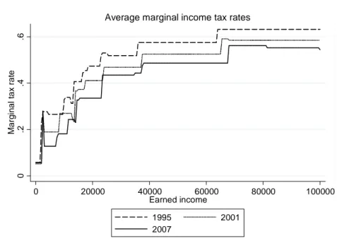
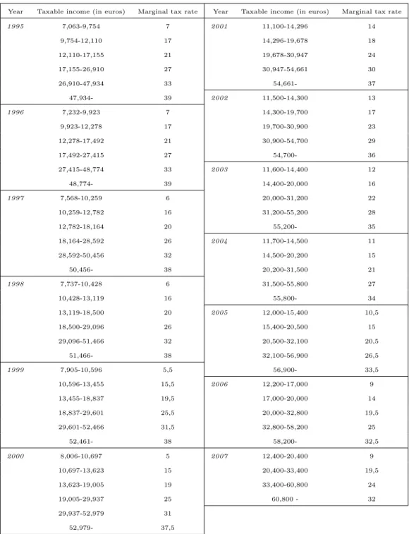
in earned income taxation that occurred in 1995-2007, since the data I use cover this time period. From the mid-1990s onwards, there has been a general decline in central government income tax rates in Finland. Central government tax rates have decreased almost every year in all income classes. Figure 1 illustrates the changes in average marginal tax rates between the years 1995, 2001 and 2007. These marginal tax rates are calculated with the average municipal income tax rate and social security contributions in the year in question. Table 4 in the Appendix presents the marginal tax rate schedule of central government income taxation in 1995-2007.
From the empirical point of view, variation stemming from changes in central government tax rates is not ideal. Although there have been significant changes in tax rates over this time period, the generally declining nature of tax rates does not provide much differential marginal tax rate variation. In relative terms, marginal tax rates declined slightly more for low and middle wage income, whereas the relative decrease was smaller in the top income bracket. This creates only small-scale variation in time in marginal tax rates for individuals at different income levels.
Municipal income taxation. Compared to central government income taxes, changes in
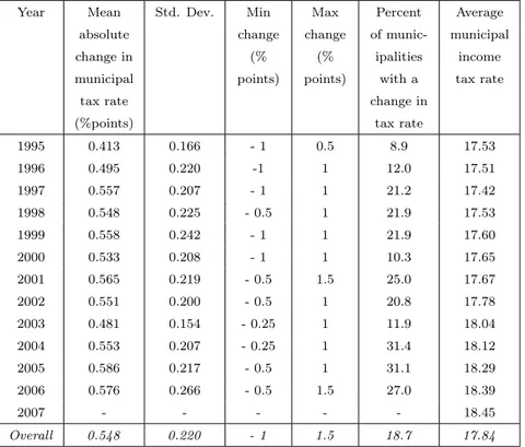
munic-ipal income tax rates have been different in nature. In Finland, municmunic-ipal tax rates have changed differently in different municipalities in different years. Table 1 presents the descriptive statistics of municipal-level tax rate changes. Depending on the year, 10-30% of municipalities have changed
3
In addition to municipal income tax revenue, the less well-off municipalities receive benefits through local tax-sharing and grants from central government. However, these are not directly related to the municipal income tax rate in the municipality in question. For example, the degree of tax-sharing depends on the industrial and demographic structure of the municipality. Within certain limits, municipalities can also charge usage fees for statutory public services, and assign low real estate taxes. In addition, part of the corporate tax revenue collected by central government is assigned to municipalities.
0 .2 .4 .6 M a rg in a l ta x r a te 0 20000 40000 60000 80000 100000 Earned income 1995 2001 2007
Average marginal income tax rates
Notes: Figure presents average marginal income tax rates at different income levels in 1995, 2001 and 2007. Marginal tax rates are calculated using average municipal income tax rates and employee social security contributions in each year. Employer pension insurance contributions are excluded.
Figure 1: Average marginal tax rates in 1995, 2001 and 2007
their tax rate. On average, every fifth municipality has changed its tax rate in each year. In all of the years in 1995-2007, at least one municipality has decreased its tax rate, and one has increased it.
One-year municipal-level tax rate changes vary from -1 to +1.5 percentage points. The average absolute change is approximately 0.5 percentage points. On average, municipal tax rates increased within the time period of 1995-2007. The average municipal income tax rate increased from 17.5% in 1995 to 18.45% in 2007.
There have also been a number of mergers (or consolidations) of two or more neighboring munici-palities. Within a merger, the merged municipalities form a new municipality and decide on a new municipal tax rate. As a consequence of mergers, the total number of municipalities decreased from 455 to 416 in 1995-2007. Table 1 does not include tax rate changes caused by municipal mergers. A more detailed discussion on using theindividual-level municipal income tax rate variation in the
Year Mean absolute change in municipal tax rate (%points) Std. Dev. Min change (% points) Max change (% points) Percent of munic-ipalities with a change in tax rate Average municipal income tax rate 1995 0.413 0.166 - 1 0.5 8.9 17.53 1996 0.495 0.220 -1 1 12.0 17.51 1997 0.557 0.207 - 1 1 21.2 17.42 1998 0.548 0.225 - 0.5 1 21.9 17.53 1999 0.558 0.242 - 1 1 21.9 17.60 2000 0.533 0.208 - 1 1 10.3 17.65 2001 0.565 0.219 - 0.5 1.5 25.0 17.67 2002 0.551 0.200 - 0.5 1 20.8 17.78 2003 0.481 0.154 - 0.25 1 11.9 18.04 2004 0.553 0.207 - 0.25 1 31.4 18.12 2005 0.586 0.217 - 0.5 1 31.1 18.29 2006 0.576 0.266 - 0.5 1.5 27.0 18.39 2007 - - - 18.45 Overall 0.548 0.220 - 1 1.5 18.7 17.84
Notes: Table presents descriptive statistics on one-year changes in municipal income tax rates from 1995-2007. Table does not include municipal mergers.
Table 1: Municipal income tax rate changes, 1995-2007
4
Data and identification
4.1 Data
I use individual-level panel data from 1995-2007, provided by Statistics Finland. The data set consists of approximately 550,000 observations per year, which constitute a representative sample of roughly 10% of the Finnish population. The data contain a wide variety of individual-level variables from different administrative registers. The main statistics used in this study are the personal tax record information provided by the Finnish Tax Administration, the Structure of Earnings statistics collected by Statistics Finland, and available municipal-level statistics.
The data set contains all the necessary information to study the elasticity of taxable income, and a substantial amount of individual and municipal-level control variables. Table 6 in the Appendix presents the summary statistics of the key variables used in this study for individuals between 25-60 years of age, including register-based variables on monthly wages, monthly working hours and tax deductions. Table 6 also includes the descriptive statistics for the key municipal-level variables.
4.2 Individual tax rate variation
The key issues in identifying ETI is the source of variation in net-of-tax rates. In short, differential variation in net-of-tax rates for otherwise similar individuals is needed when estimating ETI using individual-level panel data and tax reforms. I use changes in municipal income tax rates as the main source of this variation.4
Compared to many of the earlier ETI studies, municipal tax rate variation has some very appealing features. First, municipal tax rate changes occur in all of the years in the data (1995-2007). There are also both increases and decreases in municipal tax rates in all of the years. Second, changes in municipal tax rates affect individuals throughout the income distribution. Thus, in all income classes there are some individuals whose municipal income tax rate has changed, and some individuals faced no changes in municipal income taxation. These significantly alleviate the potential problems associated with non-tax-related changes in the income distribution, which are critical in many earlier studies that utilize changes in tax rates that occur only at certain income levels in certain years (for example one-time tax rate cuts of high-income individuals). In addition, tax rate variation across the whole income distribution identifies the parameter of main interest, the average elasticity of taxable income.
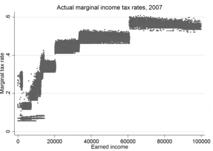
Figure 2 presents the actual individual marginal income tax rates at different income levels, highlight-ing the regional variation in marginal income tax rates. As can be seen from the Figure, individuals at the same income level face different marginal tax rates depending on the municipality of residence. Moreover, individuals with the same income level face differentchanges in overall marginal tax rates
due to differential changes in municipal tax rates over time.
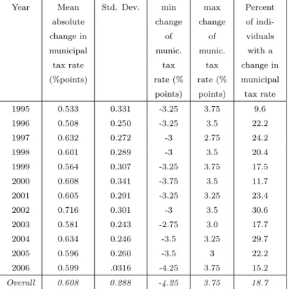
Table 2 describes the overall individual variation in municipal income tax rates. In addition to tax rate changes within a municipality, Table 2 includes individuals who faced a change in their municipal tax rate as a result of a change in their municipality of residence, or as a consequence of a merger of two or more neighboring municipalities. In the data set, 3.3% of individuals changed their municipality of residence betweent and t+ 1(on average). This number does not include mergers
of municipalities.
As can be seen from Table 2, approximately every fifth individual experienced a change in his/her municipal income tax rate each year. On average, the absolute change in the municipal tax rate was 0.6 percentage points for those individuals who faced a change in their municipal tax rate. There
4
To my knowledge, Pirttilä and Uusitalo (2005) first proposed the use of municipal income tax rate changes as a source of differential income tax rate variation in Finland.
Notes: Figure presents marginal income tax rates at different income levels in 2007. Marginal tax rates are calculated using actual municipal income tax rates, tax deductions and allowances, and employee social security contributions in each year. Employer pension insurance contributions are excluded. Marginal tax rates are calculated using an own simulation program suited for this data set, build on the basis of the Finnish JUTTA microsimulation model.
Figure 2: Actual marginal tax rates in 2007, including individual municipal income tax rates is a more distinctive difference between the smallest negative (-4.25 percentage points) and largest positive (3.75 percentage points) change in the municipal tax rate. The largest absolute changes are caused by changes in the municipality of residence. Figure 3 in Section 4.4 describes the extent of the variation for three-year difference and the baseline estimation sample excluding moving individuals. Individual changes in municipal income tax rates are not extensive in size. The majority of changes are between +/- 0.25-1 percentage points. When the whole net-of-tax rate is accounted for (municipal taxes + central government taxes + social security contributions), most of the changes are around +/- 1-10 as a percentage. The largest changes in municipal tax rates correspond to changes in overall net-of-tax rates of +/- 5-15%.
Some recent studies (e.g. Chetty (2012), Kleven and Schultz (2014)) argue that optimization frictions have an effect on the estimated taxable income elasticity. In short, if costs related to responding to tax rate changes (adjustment costs, job search costs, paying attention to tax code etc.) are large, they might attenuate the observed elasticities and make them less than the structural elasticities derived in a frictionless benchmark case.
Frictions are typically more relevant when changes in the tax rate schedule are small. Small tax rate changes might induce only small utility benefits from changing behavior, and this utility gain might be smaller than the associated (fixed) cost. Thus small changes in tax rates tend to lead
Year Mean absolute change in municipal tax rate (%points) Std. Dev. min change of munic. tax rate (% points) max change of munic. tax rate (% points) Percent of indi-viduals with a change in municipal tax rate 1995 0.533 0.331 -3.25 3.75 9.6 1996 0.508 0.250 -3.25 3.5 22.2 1997 0.632 0.272 -3 2.75 24.2 1998 0.601 0.289 -3 3.5 20.4 1999 0.564 0.307 -3.25 3.75 17.5 2000 0.608 0.341 -3.75 3.5 11.7 2001 0.605 0.291 -3.25 3.25 23.4 2002 0.716 0.301 -3 3.5 30.6 2003 0.581 0.243 -2.75 3.0 17.7 2004 0.634 0.246 -3.5 3.25 29.7 2005 0.596 0.260 -3.5 3 22.2 2006 0.599 .0316 -4.25 3.75 15.2 Overall 0.608 0.288 -4.25 3.75 18.7
Notes: Table presents descriptive statistics on one-year changes in individual municipal income tax rates from 1995-2007. Table includes changes caused by municipal mergers and moving to another municipality.
Table 2: Individual-level changes in municipal tax rates, 1995-2007
to smaller changes in observed behavior (on average).5 This is a valid point in this setup, as the
variation in overall net-of-tax rates is relatively small, at least when compared to many earlier studies. Therefore, assuming that adjustment costs or other frictions matter, we would expect to get smaller ETI estimates in this study.
In addition, it might be that the short-run response to a small change in the net-of-tax rate differs significantly from the longer-run effect. For example, the adjustment process might take more than 1-3 years, particularly if the short-run gains from the behavioral response are relatively small. In the empirical part, I test the effect of changing the time horizon on the elasticity estimate.
Finally, as highlighted by Kopczuk (2005), changes in the tax base and the definition of taxable income affect the ETI estimate. In Finland, the earned income tax base has remained relatively constant in 1995-2007. Furthermore, the minor changes in the tax base are to a large extent unrelated to the main source of tax rate variation. This is due to the fact that the tax base and basic rules of municipal income taxation, including tax deductions and allowances, are regulated at the central government level.
5Using Danish data, Chetty et al. (2011) and Kleven and Schultz (2014) show evidence that the observed elasticity
4.3 Net-of-tax rate instrument
In a progressive income tax rate schedule, the marginal tax rate increases as taxable income increases. Therefore, a change in taxable income endogenously defines the change in the net-of-tax rate, and thus a valid instrumental variable for(1−τ) is required.
A common strategy in the earlier literature is to simulate predicted (or synthetic) net-of-tax rates, and use them as instruments for the actual net-of-tax rate changes (see Gruber and Saez (2002)). The basic structure of the predicted net-of-tax rate instrument is the following: take base-year t
income and use it to predict the net-of-tax rate for t+k by using tax legislation in t+k. The
instrument for the change in the net-of-tax rate is then the difference between the actual net-of-tax rate intand the net-of-tax rate calculated with income intand the tax law fort+k. The intuition
is that the predicted difference describes the exogenous change in the tax rate caused by changes in tax legislation, ignoring any behavioral effects by keeping taxable income constant at the base-year level.
However, the predicted net-of-tax rate variable is a function of individual taxable income in yeart,
and there is no proof that this instrument is exogenous in the empirical model. Following Blomquist and Selin (2010) and Moffit and Wilhelm (2000), it is unlikely that the predicted net-of-tax rate instrument is correlated similarly with bothεt+k,iandεt,i in equation (3), as taxable income in year
tdefines the marginal tax rate in both t and t+k. In addition, there is no general proof that the
usually added controls, mainly base-year taxable income, correct this endogeneity problem (Weber (2014)). In all occasions there is concern about the validity of instruments that are functions of the dependent variable.6
In this study I use an instrument for net-of-tax rate changes which is not a function of taxable income, namely changes in flat municipal income tax rates. As the municipal income tax rate is flat, the tax rate is the same in all income classes within each municipality. In other words, at the individual level, the only determinant of the municipal income tax rate is the municipality of residence.7
6In Blomquist and Selin (2010), the middle-year characteristics (i.e. (t+ (t+k))/2) are used to define imputed
taxable income for bothtand t+k, from which the net-of-tax rate instrument is then calculated. Blomquist and Selin (2010) show that this strategy produces exogenous instruments under certain general assumptions about the autoregressive structure of the transitory income component. Weber (2014) shows that using lagged income (t−1,
t−2 etc.) enhances the validity of the predicted instrument. Nevertheless, the validity of these types of predicted net-of-tax rate instruments still depends on the serial correlation pattern ofεt,i.
7
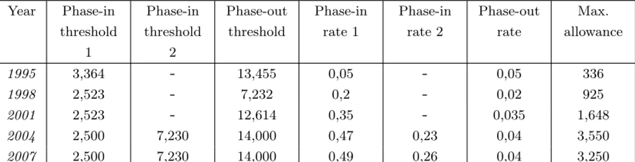
The earned income tax allowance in municipal taxation depends (inversely) on earned income. This mainly affects low-income individuals. The effect of the allowance on the effective overall net-of-tax rate is trivial for taxable income over 14,000 euros. The earned income tax allowance in municipal taxation is described in Table 5 in the Appendix.
Compared to predicted net-of-tax rate instruments, the municipal tax rate instrument has several advantages. First, I do not have to make assumptions about the time structure of the individual transitory income component in order to ensure the exogeneity of the instrument. Second, as mu-nicipal income tax rates affect the net-of-tax rates in all income classes, I do not have to explicitly control for the non-tax-related changes in the income distribution in order to guarantee the causal-ity of the behavioral parameter. Third, mean reversion does not pose a notable problem, as yearly fluctuation in individual income does not affect the instrument.
However, even though the municipal tax rate instrument is not a direct function of the dependent variable in any period, there are some concerns that the instrument might not be exogenous as such. One concern is the possible policy endogeneity of municipal tax rate changes. Municipalities might increase tax rates because of decreased tax revenue. For example, this could be caused by decreased employment in the jurisdiction. Because low employment might also decrease average individual taxable income, the elasticity estimate could be upward-biased.
In Figure 4 in Section 4.4, I test the supposition that future tax increases (or decreases) are sig-nificantly more common when individual taxable income has decreased in the past. The Figure highlights that this baseline policy endogeneity is not driving the results in this paper. Nevertheless, in order to alleviate potential policy endogeneity, I include various municipal-level covariates to the model, such as municipal-level unemployment and employment rates and the level of net debt (per capita). These variables have a presumable effect on total taxable income within a municipality, as well as average individual taxable income. By including a set of municipal-level covariates and regional income trends in the model, I can, at least to a sufficient extent, separate the possible municipal and other regional-level effects from the individual-level behavioral responses.
Another concern is the possibility that individuals select into the “treatment” by changing their municipality of residence. First, we might worry that individuals consistently move to municipalities with lower (or higher) tax rates. However, with regard to identification in the ETI model, this is not very relevant in itself.8
A more serious concern would be that changes in taxable income are systematically correlated with
8
For example, if an individual moves to a municipality with a lower tax rate but does not change his/her current job (or more precisely, taxable income does not change), ETI for this individual will be zero by definition, even though the total income taxes paid are now lower than before. Thus, this kind of purely tax-motivated migration is not an issue in this framework. Also, we might suspect that there is a classical selection problem in equation (2). The conceivable selection bias comes from the possibility that individuals who prefer low income taxation choose to reside in a municipality with a low tax rate. Preference for low income taxation is likely to be positively correlated with taxable income, causing the elasticity estimate to be biased. However, as the empirical model in question is identified by individual changes in both municipal tax rates and taxable income, this is not a very serious concern.
the moving decision, and especially with the municipal tax rate in the destination municipality (i.e. the tax rate instrument would be correlated with the transitory income component). For example, a new, better paid job might be a good reason for moving to another municipality. At the same time, it could be that municipalities with a lot of open highly paid vacancies have a relatively low or high municipal tax rate, which would bias the elasticity estimate. This is a relevant concern in the Finnish case, as the municipal income tax rates are typically below the average in high-wage regions such as the capital city area (Helsinki-Espoo-Vantaa-Kauniainen).
Therefore, in the baseline empirical specification, I drop individuals who change their municipality of residence between t and t+k in order to avoid mechanical correlation between the instrument
and the transitory income component. The downside of this approach is that it does not take into account the potential but somewhat unlikely effect of moving and decreasing (increasing) income
because of a municipal tax increase (decrease) in the base-year municipality of residence. In other words, the model excluding individuals with changes in the municipality of residence does not include all imaginable behavioral margins.
Overall, utilizing changes in flat municipal income tax rates provides a new way of constructing instruments for the changes in net-of-tax rates which avoids many of the critical issues related to income-based predicted net-of-tax rates. However, applying regional variation arguably requires more detailed consideration of regional income trends and other regional characteristics. I further study the significance of different controls in Section 5. In addition, in Section 5.2, I use the standard predicted net-of-tax rate instrument proposed in Gruber and Saez (2002), and the modified instrument using lagged base-year income proposed in Weber (2014) to estimate ETI in Finland.
4.4 Descriptive statistics
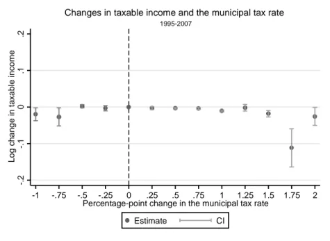
Figure 3 describes the relationship between changes in taxable income and changes in municipal tax rates. In the Figure, I plot the coefficients from a regression where I regress log changes in individual taxable income with dummy variables of different percentage point changes in the municipal tax rate using three-year differences and controlling for county-year fixed effects. The dummy variable for zero changes in the municipal tax rate is omitted from the regression. Thus in the Figure, the point on the vertical dash line denotes the omitted zero changes, which represent the comparison group to other percentage point changes in municipal tax rates.
larger the positive changes in municipal tax rates are. In other words, positive changes in municipal tax rates induce negative changes in taxable income. This reduced-form type evidence indicates that individuals respond to incentives created by changes in municipal tax rates.9 In addition, Figure 3
graphically illustrates the extent of municipal tax rate variation for the baseline estimation sample included in the Figure.
-. 2 -. 1 0 .1 .2 L o g c h a n g e i n t a x a b le i n c o m e -1 -.75 -.5 -.25 0 .25 .5 .75 1 1.25 1.5 1.75 2 Percentage-point change in the municipal tax rate
Estimate CI
1995-2007
Changes in taxable income and the municipal tax rate
Notes: Figure shows the average log changes in taxable income for different percentage-point changes in municipal tax rates. Figure presents the averageαjcoefficients and 95% confidence intervals from a regression4ln(T I)t,i=γ+P2j=−1αj4τj+
β(Y EARt∗COU N T Yi) +vt,i, where4ln(T I)t,iis the change in taxable income betweentandt+ 3for individualiand4τj
denote dummy variables for different percentage point changes in the municipal rate betweentand t+ 3. Municipal tax rate changes occur in 0.25 percentage point intervals. Base-year county*year dummies are included to control for different income trends in different parts of the country in different years. The estimation sample includes individuals with base-year taxable income above 20,000 euros. Individuals under the age of 24 and over the age of 60 are not included in the sample, and the sample is limited to individuals whose municipality of residence and marital status are unchanged betweentandt+ 3.
Figure 3: Changes in taxable income for different changes in the municipal tax rate
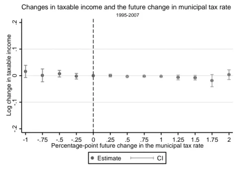
Figure 4 shows the coefficients from a regression where I regress log changes in taxable income betweentandt+ 3with differentfuture percentage point changes in the municipal tax rate between
t+ 3and t+ 6. This allows me to test whether municipal tax rate changes are determined based on
past development of individual taxable income. For example, if municipalities respond to a decrease in taxable income in the past by increasing the municipal tax rate in the future, we should see that future tax increases are significantly more common when there is a decreasing trend in average taxable income, and vice versa.
9Column (10) of Table 10 in the Appendix shows the regression results for the reduced-form model where log
changes in taxable income are regressed with log changes in the municipal net-of-tax rate using the baseline empirical specification.
Figure 4 does not support this policy endogeneity channel. There are no statistically different changes in taxable income for different future changes in the municipal tax rate. In other words, past income development is not driving the changes in municipal tax rates. Nevertheless, the point estimates are slightly more negative for larger changes in the municipal tax rate, and vice versa. Therefore, in order to take into account possible policy endogeneity, I add municipal-level covariates in the preferred empirical specification.
-. 2 -. 1 0 .1 .2 L o g c h a n g e i n t a x a b le i n c o m e -1 -.75 -.5 -.25 0 .25 .5 .75 1 1.25 1.5 1.75 2 Percentage-point future change in the municipal tax rate
Estimate CI
1995-2007
Changes in taxable income and the future change in municipal tax rate
Notes: Figure shows the average log changes in taxable income for different future percentage-point changes in munici-pal tax rates. Figure presents the average αj coefficients and 95% confidence intervals from a regression 4ln(T I)t,i =
γ+P2
j=−1αj4τjF+β(Y EARt∗COU N T Yi) +vt,iwhere4ln(T I)t,iis the change in taxable income betweentandt+ 3for
individualiand4τF
j denote dummy variables for different future percentage point changes in the municipal rate betweent+ 3
andt+ 6. Municipal tax rate changes occur in 0.25 percentage point intervals. Base-year county*year dummies are included to control for different income trends in different parts of the country in different years. The estimation sample includes individuals with base-year taxable income above 20,000 euros. Individuals under the age of 24 and over the age of 60 are not included in the sample, and the sample is limited to individuals whose municipality of residence and marital status are unchanged between
tandt+ 3.
Figure 4: Changes in taxable income and future changes in the municipal tax rate
4.5 Empirical specification
I estimate different variations of the following equation using a two-stage least squares estimator
4ln(T I)t,i =α1+e4ln(1−τ)t,i+α2Bt,i+α3Mt,m+4εt,i (4)
In equation (4), 4ln(T I)t,i is the change in taxable income between t and t+k for individual i.
net-of-tax rate. Thus e is the coefficient of interest, the average elasticity of taxable income with
respect to the net-of-tax rate. The baseline time horizon used is three years (t+ 3−t), which is
customary in the literature.
Base-year characteristics Bt,i control for observed individual and regional heterogeneity affecting
changes in taxable income. Bt,i includes year dummies, age, age squared, county of residence,
sex, level of education (highest degree), marital status, size of the household and dummy variables indicating whether the individual has received any taxable social security benefits in the base year.10
I also include interaction terms of sex and other controls in the model (age, education, household size and marital status). Importantly, I also add county-year fixed effects, which account for different income trends in different parts of the country at different times.11
To control for the possible policy endogeneity of the net-of-tax rate instrument, I add municipal-level (m) characteristics Mt,m to the estimable equation. Mt,m includes base-year values of
municipal-level employment, unemployment, net migration and net loan positions. These variables reflect the actual publicly available information that the decision-making bodies in each municipality have on the local economy.
I limit the analysis to observations where base-year taxable income is above 20,000 euros. First, as in previous ETI literature, I focus on the intensive margin behavioral responses. This emphasizes the need for a relatively large income cut-off in the Finnish context. Many of the social security benefits in Finland (e.g. unemployment benefits and sickness benefits) are regarded as taxable income, which creates relatively low but positive taxable income also for individuals fully or partly outside the labor force during the year. Second, income cut-off above 14,000 euros is needed in order to eliminate any notable effect of the municipal earned income tax allowance on the net-of-tax rate instrument. The allowance depends inversely on income, and therefore cause a mechanical correlation between income and the net-of-tax rate for low-income individuals.
In addition, I drop people under the age of 24 and over the age of 60 out of the estimation sample. Also, following earlier literature (e.g. Gruber and Saez (2002)), the analysis is limited to individuals whose marital status is unchanged between the two years. Finally, in the baseline analysis, I drop individuals who change their municipality of residence between t and t+k. However, the sample
10
Social security benefits include unemployment benefits, sickness benefits, parental leave benefits and study grants. The marital status dummies include married couples, unmarried couples, singles, divorced singles and wid-ows/widowers. There are 21 counties in Finland. Figure 5 in the Appendix presents a map of counties in Finland.
11As the variation in municipal tax rates is not based on base-year income of the individual, there is no explicit need
to include base-year (or lagged) income variables to the right-hand side of equation (4). This is a typical strategy in previous ETI literature. Also, as underlined in recent literature (see e.g. Weber (2014)), base-year income controls are endogenous and should not be included in the first place.
includes individuals whose municipality of residence changed due to a municipality merger.12
5
Results
5.1 Main results
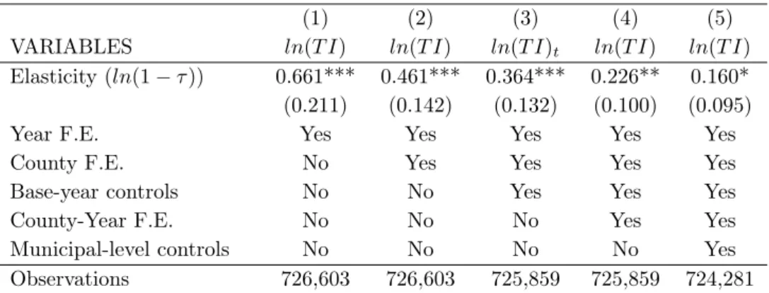
Table 3 shows the results for the three-year difference model with different specifications. First, column (1) shows the average ETI estimate with only year dummies included in the regression. This elasticity estimate is 0.66 and statistically significant at the 1% level. In column (2), I add county dummies to the estimable equation, which decreases the estimate to 0.46 and increases precision. Column (3) shows that adding individual-level base year controls further decreases the estimate to 0.36.
(1) (2) (3) (4) (5) VARIABLES ln(T I) ln(T I) ln(T I)t ln(T I) ln(T I)
Elasticity (ln(1−τ)) 0.661*** 0.461*** 0.364*** 0.226** 0.160* (0.211) (0.142) (0.132) (0.100) (0.095)
Year F.E. Yes Yes Yes Yes Yes
County F.E. No Yes Yes Yes Yes Base-year controls No No Yes Yes Yes County-Year F.E. No No No Yes Yes Municipal-level controls No No No No Yes Observations 726,603 726,603 725,859 725,859 724,281
Notes: Heteroscedasticity-consistent and municipal-level clustered standard errors in parentheses.
Table shows the results for the baseline ETI estimations. Columns (1)-(5): Equation (4) estimated using the baseline estimation sample and a three-year difference window using different sets of regional and individual control variables for 1995-2007. Baseline sample includes individuals aged 25-60 years, base-year income above 20,000€ and whose municipality of residence and marital status are unchanged betweentandt+ 3.
Table 3: ETI estimates
As discussed above, using municipal-level income tax rate variation to obtain individual-level elas-ticity estimates presumably requires more extensive regional controlling. First, column (4) adds county-year dummies to the model, which control for different income trends in different parts of the country in different years. Taking this regional heterogeneity into account decreases the elasticity estimate to 0.23.
Column (5) of Table 3 shows my preferred empirical specification with both county-year fixed ef-fects and municipal-level controls included. As mentioned before, controlling for municipal-level
12
As a sensitivity check, I also estimate the model with movers included. For the model including the movers,Bt,i
also contains a dummy variable denoting whether an individual has changed his/her municipality of residence between
characteristics is needed in order to take into account municipal-level economic circumstances that might be correlated with both changes in municipal tax rates and individual income. After adding municipal controls, the average ETI estimate is 0.16 and statistically significant at the 10% level.13
The preferred average ETI estimate of 0.16 is in line with many previous ETI studies (see Saez et al. (2012)). Furthermore, the estimate is of similar magnitude with other recent studies from the Nordic countries (e.g. Chetty et al. (2011) and Kleven and Schultz (2014) for Denmark, and Thoresen and Vattø (2013) for Norway), although the estimate is among the largest ones.14 In
general, the estimated ETI implies that marginal income tax rates have a relatively small effect on taxable income at the intensive margin. In addition, the welfare effects are moderate at the most. Using the average marginal tax rate (0.39) and the standard formula for the excess burden presented in for example Chetty (2009), the ETI estimate of 0.16 implies a marginal excess burden of around 10%.
Finally, in order to characterize the heterogeneity of the average ETI, Table 7 in the Appendix shows the results for different subgroups of taxpayers. First, columns (1) and (2) show the estimates separately for men and women. The results show that the point estimate for men (0.14) is slightly smaller than for women (0.22), indicating practically no significant differences in average responses between the sexes. Second, columns (3)-(5) show the results for low-income (10,000-25,000 euros), middle-income (25-40k) and high-income individuals (over 40k). The results show that low-income (point estimate 0.31) individuals seem to be somewhat more responsive than middle-income (0.15) and high-income (0.14) individuals. The larger estimate for low-income earners is consistent with previous literature, but the estimate in this particular context could be somewhat upwards biased due to the mechanical correlation between the earned income tax allowance and taxable income for individuals with taxable income below 14,000 €. However, in contrast to many previous studies, I do not find the ETI to be larger among high-income earners compared to middle-income individuals.
13
The F-statistics for the first stage of the two-stage least squares routine are very large and highly significant in all specifications. The first-stage result for the preferred specification is presented in column (9) of Table 10 in the Appendix.
14One potential reason for the slightly larger point estimate is the different identification strategy. Instead of using
the predicted net-of-tax rate, I use changes in flat municipal tax rates as the net-of-tax rate instrument. If the predicted net-of-tax rate instrument provides downwards-biased estimates, it is likely to receive smaller estimates when using this instrument. However, it could be that the estimated average ETI in this study would decrease if, for example, additional municipal-level controls were available, but it is in general very difficult to conjecture the potential effect possible omitted controls on the estimate.
5.2 Alternative specifications and robustness checks
5.2.1 Subcomponents of taxable income
In addition to average ETI, extensive register data allow me to characterize the structure of the overall elasticity by studying how the subcomponents of ETI, such as working hours and deduction behavior, react to changes in tax rates. Currently, there are only a limited number of studies available that systematically analyze the responsiveness of different components of ETI.15 However, detailed
knowledge of “the anatomy of behavioral response” (Slemrod (1996)) is useful when designing an income tax system and the detailed structure of tax reforms, especially in the light of minimizing the excess burden of income taxation. It is rather difficult for the policymaker to influence deep individual utility arguments, such as the opportunity cost of working (Piketty et al. (2014)). However, for example, it is easier to influence tax deduction behavior through minor adjustments to regulations. Table 8 in the Appendix presents the results for the subcomponent analysis. First, column (1) shows the elasticity of gross earned income subject to taxation. Compared to taxable income, gross earned income is a broader income concept, as it is subject to less deductions. The point estimate for the gross earned income elasticity is 0.14, which is slightly smaller than the baseline ETI estimate of 0.16. This tentatively suggests that tax deductions are responsive to changes in tax rates.
Second, columns (2) and (3) present the estimates for monthly wages and monthly working hours, respectively. Data on wages and hours come from the Structure of Earnings statistics collected by Statistics Finland. Monthly wage rates include both regular and irregular earnings, and monthly working hours include regular hours and overtime working hours. The point estimates for both the wage rate and working hours are negative and insignificant. This suggests that both work effort and labor supply are not responsive to income taxation.
However, the estimates for monthly wages and working hours need to be interpreted with caution. First, register-based information on monthly wages and monthly hours are reported to Statistics Finland by a selected sample of employers with more than five workers. Second, the information on working hours and wages is collected only for full-time workers. Third, reported working hours
15Blomquist and Selin (2010) estimate the elasticity of the hourly wage rate in Sweden, and find a significant wage
rate response. Doerrenberg et al. (2014) show that tax deductions are responsive to tax rate changes in Germany. Also, Kleven and Schultz (2014) report that capital income components of taxable income are more responsive than earned income in Denmark. Previous US literature shows that a large proportion of the behavioral response of high-income individuals has been in the form of tax avoidance via high-income-shifting (see for example Saez et al. (2012)). Harju and Matikka (2014) show that a similar result holds for the owners of non-listed businesses in Finland. In addition, the US literature has shown that charitable giving, which is tax deductible in the US, responds to changes in marginal tax rates (see for example Bakija and Heim (2011)).
and monthly wages might not precisely measure the actual working hours or wage rates of each individual worker, especially if wages are not directly based on actual hours worked (for example for workers with a fixed monthly salary with no overtime compensations). In addition, wage rates and working hours are mainly based on the situation in October in each year, which might not reflect the actual yearly responses, especially with respect to more irregular components such as overtime work. Nevertheless, given the limitations of the Structure of Earnings data, I find no evidence of significant effort (wage rate) or labor supply (working hours) responses to tax rate changes.
To further study the potential effect of other components, I estimate elasticities for fringe benefits and specific tax deductions. The data on taxable fringe benefits and tax deductions come from the Finnish Tax Administration. Column (4) of Table 8 presents the elasticity estimate for taxable fringe benefits. The responsiveness of fringe benefits seems to be relatively large (elasticity of 0.53), although the effect is imprecisely measured. This evidence tentatively supports the view that the response might come through more irregular earnings channels.
Columns (5) and (6) show the estimates for work-related expense and commuting expense deductions. Work-related expense deductions and commuting deductions are described in detail in Table 9 in the Appendix. Both deductions appear to be moderately responsive, but the estimates are again insignificantly different from zero (due to the relatively small number of available observations in the data). The signs of both deduction responses are intuitive, however. Basic taxable income theory predicts that the amount of tax deductions will increase as the net-of-tax rate decreases, and vice versa. Overall, given the data limitations, this evidence together with the relatively large fringe benefit response tentatively indicate that the overall ETI is driven by tax deduction behavior and irregular earnings rather than conspicuous changes in labor supply or work effort.
5.2.2 Robustness checks
Table 10 in the Appendix presents the results for robustness and sensitivity checks for the baseline ETI model in column (5) of Table 3. First, column (1) of Table 10 shows the estimate for the baseline specification including individuals who move from one municipality to another betweent
andt+ 3. The ETI estimate increases to 0.56 when movers are included in the sample. This implies
notable effects for individuals who changed their municipality of residence. As mentioned in Section 4.3, the elasticity estimate is presumably larger for movers due to mechanical correlation between the instrument and transitory income. As a further robustness check, I also estimate the model
without individuals who move to the largest county in Finland, which includes the capital city area (Uusimaa). The average point estimate for this model is 0.40, which is lower than the estimate when all movers are included. This supports the notion that mechanical correlation between the lower-than-average municipal tax rates and higher wage levels in larger cities bias the results when moving individuals are included to the model.
Column (2) shows the elasticity estimate with base-year taxable income weights. Income-weighting is used in many earlier ETI studies (see for example Gruber and Saez (2002)). The income-weighted point estimate (0.15) does not significantly differ from the unweighted baseline estimate. Column (3) shows the ETI estimate when the base-year income cut-off is lowered from 20,000 € to 15,000 €. The estimate with the lower cut-off increases slightly to 0.20, but the difference is not statistically significant.
Columns (4) and (5) present the results for one-year and five-year differences, respectively. The ETI estimate for the one-year difference model is 0.01. This implies that a one-year difference is too short to estimate the effect of changes in net-of-tax rates on changes in taxable income in this context. The estimate for the five-year difference model is similar in size (0.11) to the baseline three-year model. However, the estimate is more imprecise. These results imply that the baseline three-year estimation window is long enough to capture potential changes in behavior but not too long to lose identifying variation, which tends to weaken when longer time periods are used. The latter is especially relevant when using the relatively small changes in municipal tax rates as the identifying variation.
Columns (6) and (7) estimate the model using predicted net-of-tax rate instruments typically used in the literature. Column (6) shows the estimate when using the standard Gruber and Saez (2002) type predicted net-of-tax rate instrument discussed above in Section 4.3. Similarly as in Blomquist and Selin (2010), I get a negative point estimate when applying this instrument (-0.10). Column (7) shows the results for a model where income variables from periodt−1are used to calculate the
net-of-tax rate instrument, as opposed to base-year t income in the standard predicted net-of-tax
rate instrument. This alternative strategy is proposed in Weber (2014). The point estimate for this model is also negative (-0.41), and more imprecisely measured than with the Gruber and Saez instrument. The sample in these estimations is limited to observations where all the instruments (Gruber and Saez, Weber, municipal instrument) are non-missing.
The results when using the predicted net-of-tax rate instruments imply that the negligible variation in progressive central government tax rates is not suitable for identifying behavioral responses. As
shown in Table 4 in the Appendix, central government income tax rates have decreased in all income classes in a similar manner. However, the relative tax decrease was slightly larger for middle and low-income earners compared to high-income earners. Thus we get biased elasticity estimates if high-income earners have even slightly faster non-tax-related income growth that we cannot fully take into account in the identification strategy.16 This is a particular issue for predicted net-of-tax
rate instruments that are based on base-year or lagged taxable income. This issue is also supported by the data. The estimates derived using predicted net-of-tax rate instruments increase markedly when I drop individuals with taxable income over 45,000 € in the base-year from the estimation sample. For this sample the point estimate is 0.05 for the Gruber and Saez instrument and -0.19 for the Weber instrument. This evidence indicates that the counterintuitive negative elasticity is mostly driven by high-income earners in the top tax bracket. In comparison, the ETI estimates are similar for middle-income and high-income individuals when using the municipal tax rate instrument which is unrelated to individual taxable income (see Table 7 in the Appendix). To summarize, these observations demonstrate the issues related to income-based predicted net-of-tax rate instruments, and highlight that the municipal tax rate variation is the principal source of identifying tax rate variation in the Finnish context.
Finally, columns (8)-(10) show the OLS, first-stage and reduced-form results, respectively. First, column (8) shows that the OLS estimate for the ETI model provides a highly counterintuitive result with a large negative point estimate (-2.8), which highlights the need for a valid instrumental variable. Column (9) shows that the first-stage results are strong. The first-stage estimate implies that a 1% increase in the municipal tax rate accounts for a 1.5% increase in the overall net-of-tax rate. Given the general pattern of the central government tax rate changes and the three-year time window, this estimate is reasonable in size. Also, as mentioned before, the F-test statistics for the first-stage models are large and highly significant in all specifications (234 in column (9)). Column (10) shows the result for the reduced-form model where log changes in taxable income are regressed directly with the log changes in the net-of-municipal tax rate. The results show that, on average, individuals respond changes in the municipal tax rate.
16As in many other countries, the income shares of high-income individuals have in general increased in Finland in
6
Conclusions
In this study I analyze the key tax policy parameter, the elasticity of taxable income (ETI), using Finnish panel data from 1995-2007. I use variation in flat municipal income tax rates as an instrument for the changes in overall net-of-tax rates. The flat municipal tax rate is not a function of individual taxable income in any period. Also, changes in municipal income tax rates occur throughout the income distribution. Therefore, using the municipal tax rate instrument overcomes many critical issues in earlier studies, such as non-tax-related changes in the shape of the income distribution and mean reversion of income. The novel approach of utilizing changes in municipal tax rates illustrates that different institutional features can provide useful and practical identifying variation in terms of estimating sufficient statistics for welfare analysis.
My preferred estimate for the average ETI in Finland is 0.16. The preferred empirical specification includes extensive regional and municipal-level controlling. In addition, I present graphical evidence showing that potential policy endogeneity of municipal income tax rate changes is not driving the results.
The preferred estimate is in line with many previous studies from other countries, including recent evidence from other Nordic countries (Sweden, Norway, Denmark). However, the estimate is among the largest ones for the Nordic countries. Overall, using an alternative identification strategy, this study confirms the observation from earlier studies that ETI can be relatively small even if the average marginal tax rate is high. In addition to individual preferences, this is likely driven by a broad tax base and relatively limited opportunities for tax avoidance and evasion for regular income earners in Finland, as well as in other Nordic countries (see Kleven (2014)).
As an additional analysis, I provide tentative evidence that working hours and wage rates respond less than tax deductions and more irregular forms of compensation such as fringe benefits. This suggests that the overall behavioral response is not driven by profound economic parameters such as the opportunity cost of working. However, the results from the subcomponent analysis need to be interpreted with caution. It is possible that register-based data on working hours and wage rates are not sufficient to adequately measure the labor supply margin. Thus, in future work, we need richer data on various behavioral margins in order to provide more accurate conclusions on the effect of different types of behavioral changes on the overall elasticity of taxable income.
*Acknowledgments
Many thanks to Jarkko Harju, Markus Jäntti, Tuomas Kosonen, Claus Thustrup Kreiner, Teemu Lyytikäinen, Jukka Pirttilä, Marja Riihelä, Friedrich Schneider, Håkan Selin, Jeffrey Smith, Roope Uusitalo and Trine E. Vattø for their useful comments and discussion. I also thank participants in many conferences and seminars for their helpful comments. All remaining errors are my own. Funding from the Academy of Finland, Finnish Cultural Foundation, Nordic Tax Research Council, Emil Aaltonen Foundation and OP-Pohjola Group Research Foundation is gratefully acknowledged.
References
[1] Aarbu, Karl and Thor Thoresen. (2001). Income responses to tax changes – evidence from the Norwegian tax reform. National Tax Journal, 54(2): 319–334.
[2] Bakija, Jon and Bradley Heim. (2011). How does charitable giving respond to incentives and income? New estimates from panel data. National Tax Journal, 64(2): 615–650. [3] Blomquist, Sören and Håkan Selin. (2010). Hourly wage rate and taxable labor income
responsiveness to changes in marginal tax rates. Journal of Public Economics, 94(11-12): 878–889.
[4] Chetty, Raj. (2012). Bounds on elasticities with optimization frictions: A synthesis of micro and macro evidence on labor supply. Econometrica, 80(3): 969–1018.
[5] Chetty, Raj. (2009). Is the taxable income elasticity sufficient to calculate the dead-weight loss? The implications of evasion and avoidance. American Economic Journal: Economic Policy, 1(2): 31–52.
[6] Chetty, Raj, John Friedman, Tore Olsen and Luigi Pistaferri. (2011). Adjustment costs, firm responses, and micro vs. macro labor supply elasticities: Evidence from Danish tax records. Quarterly Journal of Economics, 126(2): 749–804.
[7] Doerrenberg, Philipp, Andreas Peichl and Sebastian Siegloch. (2014). Sufficient statistic or not? The elasticity of taxable income in the presence of deduction possibilities. IZA Discussion Paper No. 8554.
[8] Feldstein, Martin. (1999). Tax avoidance and the deadweight loss of the income tax. Review of Economics and Statistics, 81(4): 674–680.
[9] Feldstein, Martin. (1995). The effect of marginal tax rates on taxable income: A panel study of the 1986 Tax Reform Act. Journal of Political Economy, 103(3): 551–572. [10] Fuest, Clemens, Andreas Pei