Performance Comparison of 3D Sinc Interpolation for fMRI Motion Correction by Language of Implementation and Hardware Platform

(1)

Scholarship@Western

Electronic Thesis and Dissertation Repository

12-13-2013 12:00 AM

Performance Comparison of 3D Sinc Interpolation for fMRI

Motion Correction by Language of Implementation and Hardware

Platform

Andrew B. Kope

The University of Western Ontario

Supervisor Mark Daley

The University of Western Ontario Graduate Program in Computer Science

A thesis submitted in partial fulfillment of the requirements for the degree in Master of Science © Andrew B. Kope 2013

Follow this and additional works at: https://ir.lib.uwo.ca/etd

Part of the Computer Sciences Commons

Recommended Citation Recommended Citation

Kope, Andrew B., "Performance Comparison of 3D Sinc Interpolation for fMRI Motion Correction by Language of Implementation and Hardware Platform" (2013). Electronic Thesis and Dissertation Repository. 1836.

https://ir.lib.uwo.ca/etd/1836

This Dissertation/Thesis is brought to you for free and open access by Scholarship@Western. It has been accepted for inclusion in Electronic Thesis and Dissertation Repository by an authorized administrator of

(2)

LANGUAGE OF IMPLEMENTATION AND HARDWARE PLATFORM

by

Andrew Kope

Graduate Program in Computer Science

A thesis submitted in partial fulfillment of the requirements for the degree of

Master of Science

The School of Graduate and Postdoctoral Studies The University of Western Ontario

London, Ontario, Canada

(3)

ii

Abstract

Substantial effort is devoted to improving neuroimaging data processing; this effort however,

is typically from the algorithmic perspective only. I demonstrate that substantive running

time performance improvements to neuroscientific data processing algorithms can be realized

by considering their implementation. Focusing specifically on 3D sinc interpolation, an

algorithm used for processing functional magnetic resonance imaging (fMRI) data, I compare

the performance of Python, C and OpenCL implementations of this algorithm across multiple

hardware platforms. I also benchmark the performance of a novel implementation of 3D sinc

interpolation on a field programmable gate array (FPGA). Together, these comparisons

demonstrate that the performance of a neuroimaging data processing algorithm is

significantly impacted by its implementation. I also present a case study demonstrating the

practical benefits of improving a neuroscientific data processing algorithm's implementation,

then conclude by addressing threats to the validity of the study and discussing future

directions.

Keywords

Functional Magnetic Resonance Imaging, 3D Sinc Interpolation, Benchmarking, Parallel

Programming, OpenCL, Graphics Processing Unit, Field Programmable Gate Array, Motion

(4)

iii

Acknowledgments

I would like to thank my supervisor Mark Daley for his guidance and feedback throughout

my master’s degree, and acknowledge Conor Wild for his assistance with the evaluation of

my implementations of 3D sinc interpolation in the context of a practical motion correction

(5)

iv

List of Tables

Table 1: Workstation desktop test bed specifications. ... 30

Table 2: Laboratory desktop test bed specifications. ... 31

Table 3: Rack-mount server test bed specifications. ... 31

Table 4: Legacy laptop test bed specifications. ... 31

(9)

viii

List of Figures

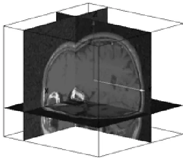
Figure 1: MRI brain image. ... 2

Figure 2: Trilinear interpolation (Wikipedia). ... 8

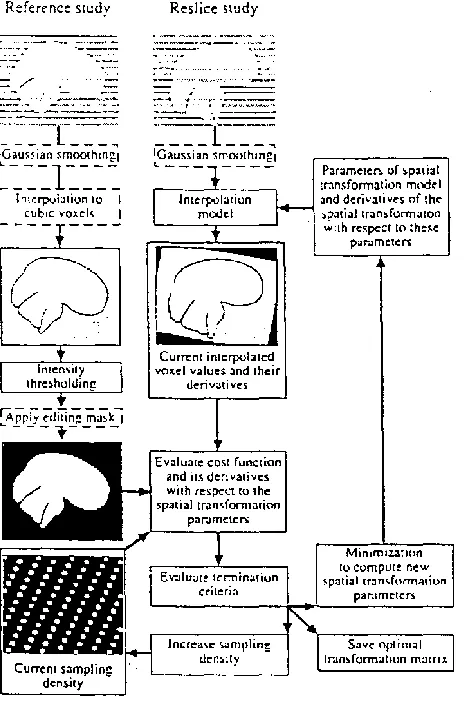
Figure 3: AIR registration algorithm (Woods et al., 1998)... 9

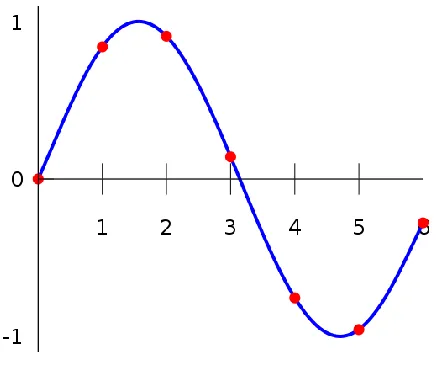
Figure 4: 1D Polynomial interpolation (Wikipedia). ... 11

Figure 5: 3D Cubic spline interpolation (GNU Octave). ... 12

Figure 6: PACE flowchart (Thesen, Heid, Mueller & Schad, 2000). ... 16

Figure 7: FSL global-local optimization ... 18

Figure 8: Illustration of a 4 x 4 x 4 sinc kernel. ... 23

Figure 9: Amdahl's Law for 50%, 75%, 90% and 95% parallelized algorithms. ... 26

Figure 10: Python implementation running time comparison across test beds. ... 32

Figure 11: C implementation running time comparison across test beds. ... 33

Figure 12: OpenCL CPU implementation running time comparison across enabled processor cores. ... 35

Figure 13: Running time as a function of enabled processor cores. ... 36

Figure 14: OpenCL CPU implementation running time comparison across enabled processor cores with single-core C implementation. ... 37

Figure 15: OpenCL GPU implementation running time performance. ... 39

Figure 16: 3D sinc interpolation running time across programming language and hardware platform within test bed 1. ... 40

(10)

ix

kernel size 13 x 13 x 13. ... 44

Figure 19: 3D sinc interpolation running time across programming language and hardware

platform within test bed 1, including the FPGA dynamic sinc kernel. ... 45

Figure 20: Wild and Cusack's robust motion correction algorithm flowchart. ... 48

Figure 21: RMC robust motion correction algorithm performance comparison within test bed

(11)

x

List of Appendices

Appendix A: List of software packages and version numbers. ... 59

Appendix B: 3D sinc interpolation mean running time across programming language and

hardware platform within test bed 1 data table. ... 60

Appendix C: Python implementation mean running time comparison across hardware

architecture data table. ... 61

Appendix D: C implementation mean running time comparison across hardware architecture

data table. ... 62

Appendix E: OpenCL CPU implementation mean running time comparison across enabled

processor cores data table. ... 63

Appendix F: OpenCL GPU implementation mean running time performance data table. ... 64

Appendix G: FPGA sinc interpolation mean running time raw data table for static and

(12)

xi

Preface

Within neuroscience, there is substantial effort devoted by researchers to the improvement of

neuroimaging data processing. This effort however, is typically only from the algorithmic

perspective with little attention paid to the hardware platform or programming language used

for the implementation of any particular algorithm. In my thesis, I demonstrate that

substantive improvements to the running time performance of a neuroscientific data

processing algorithm can be realized by giving consideration to its implementation.

I begin in Chapter 1 with a review of the physics underlying the functional magnetic

resonance imaging (fMRI) technique, followed by an overview of fMRI motion correction.

Motion correction is a preprocessing algorithm used to correct errors in fMRI data caused by

motion in the subject of the scan.

In Chapter 2, I provide a survey of several different interpolation methods used in the

performance of fMRI motion correction. For each interpolation method, I provide an

example of a popular software package which employs it in its motion correction utility.

In Chapter 3, I focus my discussion on the 3D sinc interpolation method, providing a detailed

description of the algorithm alongside a discussion of both serial and parallel

conceptualizations of it. 3D sinc interpolation provides highly accurate interpolations of

fMRI data, however its substantial running time limits its applicability; for these reasons, I

chose 3D sinc interpolation for my demonstration of the performance improvements which

can be realized by considering the hardware platform and programming language used to

implement an algorithm.

In Chapter 4, I quantify these improvements by benchmarking the performance of the 3D

sinc interpolation algorithm in Python, C, OpenCL (Open Computing Language) for

CPU/GPU across several different test bed hardware platforms. The benchmarking results

demonstrate that parallel implementations can greatly improve the running time performance

of the 3D sinc interpolation algorithm.

In Chapter 5, I describe a novel implementation of 3D sinc interpolation on a field

(13)

xii

performance improvements by showing the corresponding decrease in running time of an

algorithm for robust fMRI motion correction developed by my collaborators. I first explain

their algorithm in detail and then show the results of performance benchmarking

demonstrating these benefits.

In Chapter 7 I conclude by addressing threats to the validity of my results and discussing

(14)

Chapter 1

1

Functional Magnetic Resonance Imaging

Functional Magnetic Resonance Imaging (fMRI) is one of the foremost neuroscientific

imaging modalities in use today. This imaging technique uses the natural magnetic

properties of the human body to capture both structural images of the brain's anatomy and

functional images of its activity. fMRI is however vulnerable to errors introduced by even

slight motion in the subject of the scan; as such, motion correction algorithms have been

developed to correct for these errors. In this chapter a brief explanation of the physics

behind Magnetic Resonance Imaging is provided alongside an outline of the structure of

a general motion correction algorithm and an explanation of related concepts and

terminology.

1.1 Magnetic Resonance Imaging Physics

Magnetic resonance imaging (MRI) is a medical imaging technique which works by

taking advantage of the nuclear magnetic resonance (NMR) of the Hydrogen atoms inside

the human body. During an MRI scan, the subject of the scan is placed into a very strong

magnetic field imposed by a superconducting electromagnet which aligns the

magnetization of the Hydrogen nuclei (protons) in the water molecules within her body.

Secondary magnetic fields are then repeatedly applied to the subject by the scanner's

magnetic gradient coils, combined with strong radio frequency (RF) pulses which alter

the alignment of these magnetized protons; when the protons in the subject's tissues

return to their previous alignment a response radio frequency signal detectable by the

scanner's RF receivers is produced. These raw RF data recorded by the scanner’s

receivers are in k-space. k-space data exist in the spatial frequency domain and so are not

readily human readable. These data are converted into image space using an inverse

Fourier transform after image acquisition in complete (Twieg, 1983).

With the ability to detect both the location and type of the tissues in the subject's body in

three dimensions, MRI scanners can be used to capture 3D images of the complex tissue

(15)

as a volume. Each volume is composed of a stack of 2D images called slices. The

minimum discrete data unit within each MRI volume is referred to as a voxel (akin to a

pixel in a 2D picture); these voxels are cubes containing only intensity data (i.e. the

voxels appear only in gray scale).

Figure 1: MRI brain image.

Functional magnetic resonance imaging uses the same physical principles underlying

structural MRI brain imaging to measure subjects' brain activity over time (hence the

term functional). The human body uses hemoglobin, the primary constituent of red blood

cells, to transport oxygen within the blood stream. Importantly, oxygenated hemoglobin

is unaffected by magnetic fields however deoxygenated hemoglobin is paramagnetic and

distorts magnetic fields. fMRI scanning measures brain activity by relying on the positive

correlation between brain activity and the presence of oxygenated hemoglobin within the

brain (Ogawa et al., 1992).

When an area of the brain is active, after approximately two seconds there is a significant

increase in the amount of oxygenated hemoglobin in the blood in that brain area,

displacing deoxygenated hemoglobin. Because this oxygenated hemoglobin is unaffected

by magnetic fields, the response RF signal returned to the fMRI scanner is stronger when

there is more brain activity and therefore more oxygenated hemoglobin in that brain

tissue; this is called the blood oxygen level dependent (BOLD) signal. The peak BOLD

(16)

activity. In order to track neuronal activation in brain tissue over time, an entire brain

volume is captured approximately every 1-2 seconds with a resolution of approximately

27mm3/voxel in 3T (tesla) fMRI research scanners. The capture of a series of many

fMRI brain volumes over time is referred to as a scanning session, with the complete

dataset from one scanning session referred to as a time series. A time series might contain

for example 800 volumes, if a brain volume is captured every 1.5 seconds and the

scanning session lasts for 20 minutes. The time between the capture of each volume is

called the time of repetition (TR) or sampling time of the scanning session; increasing the

resolution of a scan is traded for an increase in TR. It is also important to note that fMRI

scanners vary in the strength of the magnetic fields used, with 1.5-7T fields being

common among modern research scanners. With a higher magnetic field strength, the

scanner can capture brain volumes faster (i.e. with a smaller TR) or at a higher resolution.

Before fMRI brain scan data can be reviewed or analyzed, they must first be subjected to

several preprocessing steps. After the initial Fourier transform to convert raw k-space

scanner data to image space, operations to remove anatomical artifacts, remove scanner

noise and improve neuronal activation detection are typically applied (for more

information see Strother’s 2006 review of BOLD fMRI preprocessing pipelines). The

focus of the present chapter is on the processing of fMRI brain scan data to compensate

for slight involuntary head movements in the subject during the scanning session,

referred to as motion correction.

1.2 fMRI Motion Correction: Overview

Motion correction was first introduced by Jiang et al. (1995) to “reduce the effect of

subject motion during the acquisition of image data in order to differentiate true brain

activation from artifactual signal changes due to subject motion” (p. 224). Because the

observable signal changes in fMRI scanning are small, even with head movements of less

than 1mm, spurious clusters of task-related brain activation can appear (Field, Yen,

Burdette & Elster, 2000). For example, if two neighbouring voxels differ in intensity by

20%, then a motion of 10% of a voxel dimension can result in a 2% signal change,

comparable to the BOLD signal in a 1.5T fMRI scanner (Bandettini et al., 1992). In the

(17)

activation artifacts itself. Freire and Mangin (2000) for example argued that some motion

correction algorithms will actively misalign motion-free fMRI data if there is an unusual

distribution of background noise or neuronal activation. Despite these criticisms however,

motion correction is generally accepted as an integral component of any fMRI

preprocessing pipeline (Lemieux et al., 2007; Lund et al., 2005).

In actuality, motion correction is a special case of image registration. As it pertains to

MRI and fMRI data, "to register two images means to align them, so that common

features overlap" (Kostelec & Periaswamy, 2003, p. 161). One common application of

image registration for fMRI data is aligning different subjects’ brain regions to a common

anatomical template to enable comparisons between subjects in a study. In the context of

motion correction, all of the volumes in one subject’s scanning session are aligned to a

common positional template to enable comparisons between volumes across a scanning

session.

1.3 fMRI Motion Correction: General Algorithm

In the general case, the image alignment responsible for correcting motion in fMRI is

done by the iterative performance of three major steps on each volume in a scanning

session time series:

1. Determination of the difference (error) between the current image and a template

image (e.g. the first image in a scanning session) using a cost function.

2. Application of an optimization algorithm to determine a spatial transformation to

move the current image closer to the template image.

3. Interpolation of the scan data based on the spatial transformation from step two to

create a new current image for the next iteration of the algorithm.

These three steps will continue until the error determined in step one is below a threshold

determined by the optimization algorithm in step two. The error function in step one, the

optimization algorithm in step two and the interpolation method in step three are each

(18)

dimensions, outlined below are several other dimensions along which different motion

correction algorithms can vary; examples of specific motion correction algorithms

varying along these dimensions are provided in the next chapter.

First, a motion correction algorithm can work either online or offline. An online

algorithm corrects for subject motion while the scan is in progress and thus must be able

to correct the motion of one volume in less time than the TR of the scanning session. This

limits the complexity of these algorithms, however allows adjustments to the scanner

parameters to be made ‘on the fly’ to improve scan accuracy and also enables researchers

to use real time fMRI (rtfMRI) experimental and therapeutic paradigms such as

biofeedback therapy (e.g. Weiskopf et al., 2007). Offline motion correction algorithms,

conversely, are applied after the entire scanning session is complete. Because they are not

required to execute within one time of repetition cycle, offline motion correction

algorithms are able to employ much more complex, compute-intensive optimization and

interpolation algorithms and can prioritize accuracy as opposed to speed.

Another important distinction is between correcting for physiological motion versus

random motion. Physiological motion refers to the cyclical motion of the head and blood

vessels caused by respiration and pulse. Although these motions are relatively small, they

can cause significant modulation of the BOLD signal (Noll & Schneider, 1994). Random

motion refers to unintentional head movements caused by involuntary muscle twitches or

an inability to maintain a stationary head position. The magnitude of these random

movements is usually less than 1mm in normal subjects, but in certain special populations

such as infants, the elderly, or the mentally ill these motions can be up to several

millimeters (Friston et al., 1996).

It is also important to draw a distinction between volume-by-volume and slice-by-slice

motion correction. In traditional fMRI scanning, each slice of each volume is acquired in

series over time. As such, there is a choice in how many slices to treat as a unit when

registering them. In volume-by-volume motion correction, the time difference between

capturing each slice is ignored and all of the slices composing the subject's entire brain

(19)

each successive brain volume to a reference volume. The reference volume is usually the

first volume of the scanning session; an average of several volumes can however also

serve as this reference (Friston et al., 2006). Slice-by-slice motion correction, however,

operates at a finer temporal granularity. In this case, each slice (or a collection of several

slices, referred to as a chunk) is treated as a discrete unit and is aligned to a reference

slice or reference chunk. Volume-by-volume motion correction has the benefit of faster

processing time, because fewer alignments must be carried out; slice-by-slice motion

correction is however able to compensate for greater magnitudes of motion which cause

significant changes in brain position during the capture of a single volume (e.g. Speck,

Hennig & Zaitsev, 2006).

In the case of volume-by-volume and slice-by-slice motion correction, the 3D imaging

data being aligned are typically treated as a rigid body. Under the rigid body assumption,

there are only six degrees of freedom (three rotational and three translational) along

which an image can be transformed to align it with the template image. The rigid body

assumption is generally valid because the brain and head move together during scanning;

this assumption also serves to simplify the optimization step used in most motion

correction algorithms.

Finally, the spatial transformation that a motion correction algorithm produces to align a

given image back to the template image can be linear or nonlinear. Linear spatial

transformations include translation, rotation and zooming. Most linear transformations

preserve the rigid body assumption and do not deform the 3D brain image. Nonlinear

spatial transformations include affine transformations and warps; these are most often

used when registering a subject's scan data to a reference anatomical template to facilitate

between-subject comparisons. Because nonlinear spatial transformations violate the rigid

body assumption, most motion correction algorithms provide linear spatial transformation

(20)

Chapter 2

2

Interpolation Methods in fMRI Motion Correction

The interpolation method used in a given motion correction algorithm has a significant

impact on the algorithm's overall performance (Jenkinson, Bannister, Brady & Smith,

2001). Interpolation is used in fMRI motion correction both to determine the values of

voxels intermediate to the raw scan data during optimization of the spatial transformation

(or motion estimate) and to produce the final scan session data once an accurate spatial

transformation correcting for the subject motion in each volume has been determined.

The interpolation step of an iterative motion correction algorithm is also often its most

compute intensive component. Correspondingly, the speed of the interpolation method

will tend to dominate the running time performance of a motion correction algorithm; this

is especially so if the algorithm needs to perform many iterations (and therefore

interpolations) when determining an optimal spatial transformation (or motion estimate).

In this chapter, a review of several methods for the 3D interpolation of fMRI

neuroimaging data is provided; for each interpolation method, the structure of the

algorithm and a prominent software package employing it are described.

2.1 Trilinear Interpolation

Trilinear interpolation is a multivariate interpolation method which allows for the

interpolation of intermediate points on a regular 3D grid by chaining together multiple

linear interpolations. Trilinear interpolation is one of the fastest 3D interpolation methods

however it is often criticized for its potential inaccuracy.

2.1.1 Algorithm

Trilinear interpolation is algorithmically the simplest method of interpolation presented in

this chapter. Given a set of known points on a regular 3D grid, trilinear interpolation uses

a chain of 7 individual linear interpolations to approximate the value of any intermediate

point contained within a rectangular prism given by the grid. Although trilinear

(21)

disadvantage of relative inaccuracy compared to other interpolation methods (Tong &

Cox, 1999). Trilinear interpolation has also been criticized for introducing spatial

smoothing when applied to fMRI data (Oakes et al., 2005).

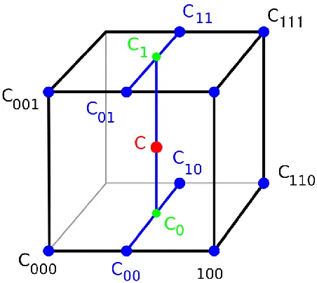
Figure 2: Trilinear interpolation (Wikipedia).

For a given intermediate point c whose value needs to be interpolated, the eight corners

of a cube on the regular grid surrounding it are first found. Then, four intermediate points

on the lines connecting those eight corners, referred to as c00 c01 c10 and c11, are calculated

using one dimensional linear interpolation. Next, two intermediate points on the lines

connecting c00 c01 c10 and c11 are interpolated, referred to as c1 and c0. Finally, c is given

by the linear interpolation of c1 and c0. These steps are shown in Figure 2.

2.1.2 AIR Software Package

In their 1998 paper, Woods et al. describe their Automated Image Registration (AIR)

software package. This package contains an image registration method which functions

very similarly to the general motion correction algorithm described in the previous

chapter. This registration algorithm serves as the foundation for the AIR software

package's motion correction utility, because as stated previously motion correction is

actually a special case of image registration. In the AIR registration algorithm an original

(22)

function is evaluated which provides the algorithm with a quantitative measure of how

well the images are registered, then finally an optimization function determines a new

spatial transformation to apply to the image for the next cycle of the registration

algorithm. A schematic of the AIR registration algorithm is shown in Figure 3.

Figure 3: AIR registration algorithm (Woods et al., 1998).

To compare the images being registered, one of the images must be resampled according

to the parameters of the current spatial transformation. This resampling requires that

voxel intensities at locations in between the voxel locations represented in the original

image be calculated. The AIR algorithm uses the trilinear interpolation method to

perform this calculation. Once the final spatial transformation has been determined on the

last iteration of the realignment algorithm, the AIR software package provides the option

(23)

To determine the error for a given iteration of the realignment algorithm, the AIR

software package uses the ratio image uniformity (RIU) cost function. To compute this

cost function, a resampled image (given by a set of realignment parameters) is divided by

the image to which it is being registered on a voxel-by-voxel basis to create a ratio image,

with the uniformity of this image measured by its standard deviation. This standard

deviation is then divided by the mean ratio to provide a normalized cost function value

for the realignment parameters used to create the image. The minimization of this cost

function therefore increases the uniformity of the ratio image independent of the global

intensity scaling of the original images. The AIR software package also includes a second

option for the cost function, namely a least squares approach similar to that used by

Friston et al. (1996). The least squares cost function is given by the average

voxel-by-voxel difference between the resampled image and the reference image. The AIR least

squares cost function also adds an intensity scaling step to compensate for global

discrepancies in image intensity.

To handle the iterative adjustment of the spatial transformation to find an optimal rigid

body transformation of the brain image, the AIR software package uses a variation on the

Powell optimization algorithm (Powell, 1964). This optimization is a conjugate direction

method, searching through a 6D parameter space to find a local minimum of the error

function used. Powell's method does not require that derivatives be taken (as does for

example the Gauss-Newton method described below), but instead minimizes the error

function using a bi-directional search along each vector in a set of search vectors, usually

simply the normals of the search space aligned along each axis. As such, it is useful for

calculating the local minimum of a continuous but complex non-differentiable function.

2.2 Spline Interpolation

Spline interpolation is a special case of polynomial interpolation, using a piecewise

polynomial called a Basis spline. Splines were originally used to describe curves in

shipbuilding and are now widely used in computer graphics. Spline interpolation is a

special case of polynomial interpolation however it has several advantages over its more

(24)

2.2.1 Algorithm

Given a set of n unique one dimensional points, the 1D polynomial interpolation problem

is to find the polynomial function which goes exactly through those points. The search

for this polynomial is equivalent to solving a linear system of equations; with a

polynomial of at least degree n - 1, there exists a provably unique solution to this linear

system. The 1D case of polynomial interpolation is shown in Figure 4.

Figure 4: 1D Polynomial interpolation (Wikipedia).

Spline interpolation is a special case of polynomial interpolation using a Basis spline

function. A Basis spline or B-spline is a piecewise polynomial function continuous at

each piece boundary, called a knot. Given a set s of n unique points, spline interpolation

will produce a piecewise polynomial function which passes through each knot point in s

while minimizing the amount of bending within the function as a whole (Webster &

Oliver, 2001). Typically, third degree polynomials are used for each piece of the function

(idem); these are referred to as cubic splines. First and second degree polynomials can

also be used however; these are referred to as linear and quadratic splines respectively.

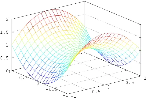
An example of 3D cubic spline interpolation from the GNU Octave software package is

(25)

Figure 5: 3D Cubic spline interpolation (GNU Octave).

Spline interpolation is generally preferred over polynomial interpolation because of the

low interpolation error which can be achieved even when using low degree polynomial

functions for each piece of the function. Spline interpolation also avoids the problem of

oscillation at the edges of the interval of interpolation, which can occur when fitting a

high degree polynomial function to a set of equally spaced data points (also known as

Runge's phenomenon; see Fornberg & Zuev, 2007).

2.2.2 SPM2 Software Package

Friston et al. present an "efficient, automatic, and general multidimensional nonlinear

spatial transformation technique" (1995, p. 166). It was the authors' intention to create a

general registration algorithm applicable for realigning variations and combinations of

fMRI, structural MRI and positron emission tomography (PET) data. In order to

accomplish this, the authors used two guiding principles in designing their algorithm.

First, the authors wanted the constraints on the image transformations their algorithm

would use to be reasonable, explicit and operationally specified. To this end, the authors

decomposed the differences between two images into two components: intensity

differences between two images which are in perfect physical alignment and differences

(26)

transformations produced by their algorithm are a nonlinear combination of rotational,

translational and intensity transformations.

The authors' second guiding principle was to develop a method with a single unique

solution transformation for each volume to be aligned. To this end, the authors linearised

the intensity transformation function using a low-order Taylor series approximation,

ensuring that a single least squares solution exists for every image registration; a least

squares solution uses an over-determined system of equations to minimize the sum of the

squares of the errors (SSE) in the results of each equation. To minimize the sum of

squared errors in the system of equations, the authors employed Gauss-Newton

optimization. The Gauss-Newton optimization method iteratively finds the minimum SSE

based on the first derivative of the sum of squared error function. This algorithm can

produce general image registration solutions, however when used for fMRI motion

correction the authors’ algorithm uses only translations, rotations and an identity intensity

transformation. That is, the solution transformation produced still follows the rigid body

assumption.

This general nonlinear registration algorithm served as the foundation of the motion

correction algorithm used in the neuroimaging data processing software package SPM2

(Statistical Parametric Mapping 2), maintained by the Wellcome Trust Centre at

University College London. SPM2 uses a registration algorithm closely based on that

presented in Friston et al.’s 1995 paper to provide estimates of subject motion, then using

those estimates determines a solution spatial transformation to correct for that motion.

Once a solution transformation has been determined, the original scan data is interpolated

using a 4D Basis spline to produce the final motion corrected scan data.

2.3 Fourier Interpolation

Fourier interpolation is lauded for combining speed and accuracy when interpolating

fMRI data. Because it operates on data in the Fourier domain, the native k-space of raw

(27)

2.3.1 Algorithm

Consider a spatial transformation which will rotate a slice from an fMRI volume. To

determine the new voxel intensities for the slice given that spatial transformation, voxel

intensity values intermediate to the existing image must be computed. Fourier

interpolation computes these intermediate voxel intensities by first converting the spatial

transformation from an image space transformation to a k-space transformation. This new

transformation is then applied to the raw k-space data and the result is used to produce

the new voxel intensities though the application of an inverse Fourier transform:

2.3.2 AFNI Software Package

Cox and Jesmanowicz (1999) describe a fast and accurate method for shifting and

rotating a 3D image using a shear factorization of the rotation matrix, as is used to handle

motion correction in the AFNI (Analysis of Functional Neuroimages) software package

(Cox, 1996). The authors based their method on the work of Eddy, Fitzgerald and Noll

(1996) who proposed the combination of three 2D shearing operations and Fourier

transform based shifting for 2D MRI rotation. The authors extended this previous work,

relying on the principle that a 3D proper orthogonal matrix can be factored into three 2D

rotations and so a general 3D image rotation can be accomplished with nine 2D shears.

As such, a 3D shear factorization has the same advantage that a 2D shear does in that its

elementary operations are coordinate shifts on 1D rows extracted from the image. In the

authors' algorithm, when any particular row of the 3D image is shifted in this way, the

row's data are interpolated using fast Fourier transforms (FFTs).

To determine the correct rotation in order to register a given volume to a template image,

the authors repeatedly linearised a weighted least squares penalty (or error) function with

respect to a rigid body transformation of the brain. This error function is:

(28)

Repeated linearization is equivalent to applying an iterative gradient descent algorithm to

the least squares penalty function. Gradient descent works by stepping toward the next

lowest point in the error space of the least squares penalty function at each iteration of the

optimization algorithm. The size of the step taken at each iteration is based on the first

derivative of the error function on that iteration. Gradient descent can work in an error

space of any number of dimensions and is guaranteed to converge to a local minimum,

however convergence can be slow close to minima because the first derivatives of the

error function surrounding them are typically small. When the error function has been

minimized, the corresponding 3D shear image rotation will align the current image to the

template image and thereby correct for subject motion.

2.3.3 PACE Motion Correction

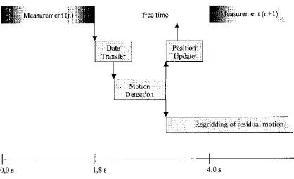
The PACE (Prospective Acquisition CorrEction) motion correction method presented by

Thesen, Heid, Mueller and Schad (2000) departs from retrospective motion correction

techniques, where motion is corrected for by processing the data after a full set of scan

data have been acquired. PACE instead corrects for motion and updates the scanner

parameters for slice orientation and position in real time after each volume is captured

(the principle flow chart of the complete PACE real-time acquisition correction is shown

in Figure 6). After each volume is acquired, the motion of that volume relative to a

reference volume is detected, then those positional data are sent simultaneously to the

scanner and to a Fourier interpolation algorithm (the authors refer to interpolation as

regridding).

To detect the motion in each volume during the scan, PACE uses as a similar technique

to Friston et al. (1996). First, one volume is chosen as a reference to which all subsequent

volumes will be aligned. To speed up computation, the PACE algorithm uses only a

subset of voxels in the brain scan to perform the alignment, covering roughly the area

containing brain tissue in the interior slices of the volume. Next, the rigid body

transformation mapping the current volume being aligned to the reference volume is

expanded as a first order Taylor series. This Taylor series is approximated and a least

squares solution for its parameter function is obtained iteratively (with the motion

(29)

algorithm produces a rotation matrix and a shift vector describing the motion between the

most recently acquired volume and the reference volume. The authors suggest that for

typical fMRI scans, the motion in any given volume can be detected with only ten

iterations of this function.

Figure 6: PACE flowchart (Thesen, Heid, Mueller & Schad, 2000).

This method of prospective motion correction feeds back the positional information

calculated from a given volume to the next volume in the scanning session, however

because of the 3-4 second delay in volume acquisition for the scanner the authors were

using, their algorithm also includes a step to remove any residual motion not corrected

for by the use of updated positional parameters during image acquisition. For each

acquired volume, the transformation required to adjust the current image to the reference

image are calculated, then this transformation is used to regrid (interpolate) the measured

volume in order to eliminate residual volume to volume motion from the final session

data. The authors chose to use Fourier interpolation, specifically the shearing method

introduced by Eddy, Fitzgerald and Noll (1996) described above to accomplish this

(30)

2.4 Sinc Interpolation

Like spline interpolation, sinc interpolation is a special case of the more general

polynomial interpolation. Sinc interpolation has the unique advantage of being able to

provide an almost perfect reconstruction of band-limited data. Although it provides high

quality results, sinc interpolation is very slow relative to other interpolation algorithms

(Friston et al., 1996).

2.4.1 Algorithm

A detailed exploration of the 3D sinc interpolation method is provided in Chapter 3.

2.4.2 FSL MCFLIRT Software Package

Jenkinson, Bannister, Brady and Smith (2001) wanted to address the problem of the

optimization method used in motion correction algorithms; a problem they argue had

received little attention at the time. Specifically, the authors argue that most optimization

algorithms in use at the time of their writing were susceptible to becoming trapped in

local minima of the so-called error space of the optimization function. That is, the

optimization algorithm might become caught in a ‘large scale basin’ or a ‘smalls scale dip’ and fail to reach a global minimum for the cost function.

In the former case, an optimization algorithm would produce a large misregistration

because the local minimum of a large scale basin is far from the global minimum. In the

latter case, the optimization algorithm simply stops prematurely at a small scale dip,

causing a large misregistration at low resolutions or a small registration at high

resolutions. To combat these two types of local minimum optimization errors, the authors

used a two-pronged approach; apodization of the cost function (that is, smoothing the

function at its edges) to eliminate the ‘small dip’ error, combined with a hybrid

global-local optimization technique which utilizes prior knowledge about the transformation

parameters and typical data size to avoid ‘large scale basin’ errors.

The mathematical details of how the authors apodized the cost function are outside the

scope of this paper, however their global-local hybrid optimization method warrants

(31)

minimum of the cost function given some time restriction. The method uses four stages

of search, each with the template and image to be aligned scaled to a different resolution

(see Figure 7). At each stage, whenever the global-local hybrid optimization method is

minimizing the cost function, Powell minimization is used.

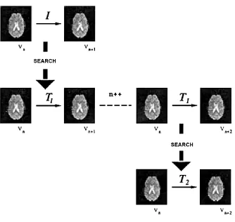
Figure 7: FSL global-local optimization

(Jenkinson, Bannister, Brady & Smith, 2001).

In the first stage, the images are pre-blurred with a Gaussian kernel and voxels are scaled

to 8 x 8 x 8mm, preserving only the gross image features. The search for a minimum of

the cost function at the 8mm stage is divided into three steps: step one, a coarse search

over the rotation parameters with a full local optimization of translation and scale for

each rotation tried; two, a finer search over rotation parameters but with only a single cost

function evaluation at each rotation; three, a full local optimization (rotation, translation

and global scale) for each local minimum detected from the previous stage (ibid., p. 831).

(32)

motion, the progression of these steps provides several reasonable potential starting

points in the error function for the next stage of the optimization.

The second stage of the optimization is performed at 4 x 4 x 4mm scale (images are again

pre-blurred with a Gaussian kernel). This stage takes the top three local minima

candidates for the global minimum, then also generates six rotational and four scale

perturbations of each of these minima, producing 33 candidate starting points for a

multi-start search of the error function space. After each of these candidate motion estimations

have been minimized for error, the single best candidate is selected for further

optimization in the next stage of the method.

The third stage of the algorithm works with the images scaled to 2 x 2 x 2mm, where

skews and anisotropic scalings begin to become significant. Consequently, the authors’

method progressively introduces these extra degrees of freedom (DOF) to the error

minimization function by calling the local optimization method three times: first using

only 7 DOF (rigid body and global scale), then with 9 DOF (rigid body and independent

scalings), then with the full 12 DOF (rigid body with scales and skews). After the

optimization has run with these additional degrees of freedom, the current motion

estimate is passed to the next stage of the method.

In the last stage of global-local hybrid optimization method, with the image scaled to 1 x

1 x 1mm, the cost function evaluations take 8 times longer than at the 2 x 2 x 2mm scale

and 512 times longer than at the 8 x 8 x 8mm scale. As such, during this stage only one

pass of the Powell local optimization algorithm is performed, the result of which is the

final registration solution.

When the global-local hybrid optimization method is applied to the problem of motion

correction, as in the FSL (fMRIB Software Library) software package’s MCFLIRT

(Motion Correction fMRIB Linear Image Registration Tool) utility, the middle image of

the scan series is taken as the template to which all other volumes are registered.

Furthermore, the final two stages of optimization at the 2mm and 1mm scale are omitted.

When the image registration transformation is computed, sinc interpolation is used to

(33)

2.5 Other Motion Correction Techniques

In this chapter several motion correction algorithms from the past 20 years have been

discussed. Most of these algorithms rely on the iterative adjustment of an estimate of

subject motion using an optimization algorithm alongside a cost function describing the

error difference between an uncorrupted image and a template image (e.g. Jenkinson,

Bannister, Brady & Smith, 2001; Thesen, Heid, Mueller & Schad, 2000; Woods et al.,

1998). Each of the algorithms relying on this optimization process to perform motion

correction varies in its computation of the cost function, the optimization algorithm used

and the nature of the estimation of the motion. Other approaches, such as predictive

approaches using a priori estimates of physiological motion are also possible (e.g.

Glover, Li & Ress, 2000; Hu, Le, Parrish & Erhard, 1995) and instead rely on removing

trends in the raw data that are correlated with known periods of subject motion.

A class of motion correction approaches which have not been reviewed here are those

which use external markers to monitor the movement of the subject's head during

scanning to provide the estimates for motion, then remove that estimated motion from the

scan data. This can be done either retrospectively after data acquisition is complete (e.g.

Tremblay, Tam & Graham, 2005) or prospectively while data is being acquired (e.g.

Zaitsev et al., 2006). Furthermore, the modality of this positional monitoring can vary,

from optical markers to track motion (as in the previous two examples) or radio

(34)

Chapter 3

3

Three Dimensional Sinc Interpolation

As demonstrated in the previous chapter, several different 3D interpolation methods are

currently in use for fMRI motion correction. Of these methods, sinc interpolation was

selected to demonstrate the importance of the programming language and the hardware

platform used for executing a neuroimaging data processing algorithm.

Sinc interpolation was chosen for this demonstration for two reasons. It is considered

among the best interpolation methods for 3D data interpolation (Tong & Cox, 1999) and

as such the development of new and faster implementations will service the

neuroscientific community. Secondly, other methods of 3D data interpolation such as

trilinear interpolation and spline interpolation have sufficiently short running times that

the differences between different implementations could be insubstantial; sinc

interpolation however has a long running time (Friston et al., 1996) and therefore would

best serve to demonstrate inter-implementation differences.

3.1 Algorithm

Sinc interpolation, also known as the Whittaker-Shannon interpolation method, is based

on the unnormalized sinc function. The term sinc is a contraction of the Latin sinus

cardinalis meaning cardinal sine, with the unnormalized sinc function is defined as

for x ≠ 0, with sinc(0) = 1. Sinc interpolation is commonly employed in digital signal

processing for the band-limited interpolation of discrete-time signals. Band-limiting is the

limiting of a signal's Fourier transform to zero above a certain finite frequency.

Band-limiting is an important concept within the context of sinc interpolation, because a

band-limited signal can be fully reconstructed from its samples, provided that the sampling

frequency exceeds twice the maximum frequency in the band-limited signal; the

(35)

referred to as the Nyquist frequency. In essence, with a band-limited signal sinc

interpolation can be used to correctly compute signal values at arbitrary continuous times

from a discrete set of samples provided they are sampled at a rate above the Nyquist

frequency. The standard sinc interpolation formula is

which can be expressed using only the sine function as

where T is the sampling period used to determine xn and x(t) is the reconstructed signal.

The above formula represents a linear convolution between the sequence and scaled and

shifted samples of the function (Oppenheim & Schafer, 1975).

Hajnal et al. (1995) describe an expansion of the standard sinc interpolation formula

allowing for the 3D interpolation of neuroimaging data. This expansion is accomplished

with a cosine Hann (Hanning) window using the normalized sinc function

In this formulation, the intensity value for a given voxel is the multiplicative combination

of three 1D sinc interpolations, with one interpolation for each dimension. The intensity

value I for voxel at (x, y, z) is defined using a Hann sinc interpolation as

with HS(a,A,R) defined as

(36)

where X,Y,Z are the coordinates of the original data set and R is the size of the Hann

window used. This Hann function eliminates problems with oscillatory effects at

discontinuities in the function and guarantees that the convolution coefficients fall off to

zero at the edge of the Hann window (Thacker, Jackson, Moriarty & Vokurka, 1999). A

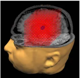
graph of the Hann window function as applied to audio samples is show in Figure 8

(Wikipedia). Throughout this document the collection of voxels in a given volume

covered by the Hann window is referred to as a sinc kernel and to the portion of the final

interpolated intensity I given by one of the voxels in a sinc kernel as that voxel's sinc

contribution. Throughout the remainder of this document, the size of a sinc kernel is

referred to by its radius; that is, a sinc kernel of size 7 x 7 x 7 will have 7 voxels between

the intermediate voxel v and an outer plane of the 3D kernel. Figure 8 below shows an

illustration of a 4 x 4 x 4 sinc kernel.

Figure 8: Illustration of a 4 x 4 x 4 sinc kernel.

The asymptotic time complexity of the serial sinc interpolation function depends on

whether the number of voxels to be interpolated or the size of the kernel is varied. In the

case that the number of voxels is varied, the sinc interpolation function has a complexity

(37)

3.2 Serial Implementation

As explained in Chapter 1, during motion correction new coordinates for each voxel in an

fMRI volume are given by the solution spatial transformation computed by the

optimization algorithm. Because these coordinates lie between the existing coordinate

grid of the raw scan data, an estimate of the intensity value for each of these intermediate

voxels must be calculated. In this section the structure and function of a serial algorithm

for the 3D sinc interpolation of the intensity at an arbitrary point within a fMRI brain

scan volume is presented, which for convenience is referred to as serialSinc. serialSinc is

based on the AIR5 3D sinc interpolation algorithm (Woods, Cherry & Mazziotta, 1992).

The serialSinc algorithm takes as input an array of coordinates, intermediate to the

existing grid structure of the raw fMRI data, whose intensity values need to be

interpolated; the input array of intermediate coordinates is referred to in serialSinc as a

chunk. The number of voxels in a chunk can vary depending on whether the motion

correction algorithm in question operates slice-by-slice, volume-by-volume, or

somewhere in between. As such, serialSinc is designed to handle an arbitrary number of

voxels per chunk. The number of voxels in the chunk is referred to as the chunk size.

serialSinc uses the Hann windowed 3D sinc interpolation method described above to

compute the new intensity value for each intermediate voxel coordinate. As explained in

the previous section, the new intensity value for a given voxel v is the sum of the sinc

contribution of each known voxel in its surrounding sinc kernel. The sinc contribution for

a given voxel in the sinc kernel is computed by multiplying its one dimensional sinc

contribution (given by the Hann windowed normalized sinc function) in each of the x, y

and z directions by its intensity. In serialSinc, the sinc contribution of each voxel in the

sinc kernel is computed serially and added to the total for the interpolated intensity of

voxel v. This total is then stored in an array holding the new interpolated intensities for

every voxel in the chunk. The size of the Hann window and therefore the size of the sinc

kernel along the x, y and z dimensions is passed into serialSinc as a parameter.

The serialSinc algorithm is shown in pseudocode below, alongside the sinc function,

(38)

// serialSinc Algorithm GET kernelSizeX GET kernelSizeY GET kernelSizeZ GET chunkXSize GET chunkYSize GET chunkZSize GET chunkCoordinates INIT interpolatedChunkIntensities

FOR kernelCenterZ in chunkZSize FOR kernelCenterY in chunkYSize

FOR kernelCenterX in chunkXSize

COMPUTE kernelBoundsX from kernelSizeX and kernelCenterX COMPUTE kernelBoundsY from kernelSizeY and kernelCenterY COMPUTE kernelBoundsZ from kernelSizeZ and kernelCenterZ

SET kernelTotal to 0

FOR currentVoxelPositionZ in kernelBoundsZ

COMPUTE sincz = sincFunction(currentVoxelPositionZ)

FOR currentVoxelPositionY in kernelBoundsY

COMPUTE sincy = sincFunction(currentVoxelPositionY) SET sinczy to (sincy * sincz)

FOR currentVoxelPositionX in kernelBoundsX

COMPUTE sincx = sincFunction(currentVoxelPositionX) SET sinczyx to (sincx * sinczy)

GET currentVoxelIntensity

SET newVoxelIntensity to (currentVoxelIntensity * sinczyx) ADD newVoxelIntensity to kernelTotal

STORE kernelTotal in interpolatedChunkIntensities // sincFunction

GET voxelPosition GET kernelCenter GET kernelSize

IF voxelPosition == kernelCenter SET result as 1.0

ELSE

SET result as sin(pi*voxelPosition)/(pi*voxelPosition) * \

0.5*(1.0 + cos((pi*voxelPosition)/kernelSize))

(39)

3.3 Parallel Implementation

Parallel computing in general is based on the principle that large computing problems can

be divided into many smaller problems, all of which can be completed simultaneously.

The two primary paradigms in parallel computing are data parallelism and task

parallelism. Task parallelism achieves improvements in the execution time of an

algorithm by running sections of it concurrently. A section of code which is designed to

run in parallel with other copies of itself is called a kernel (referred to herein as a parallel

kernel to avoid confusion with sinc interpolation kernels). Each copy of the kernel is

executed in its own thread; a serial algorithm will run in only one thread executing a

repeated section of code thousands of time in sequence, whereas a parallel algorithm

could run thousands of copies of a kernel in hundreds of threads simultaneously,

depending on the hardware architecture employed.

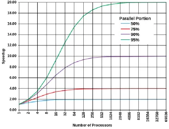
Figure 9: Amdahl's Law for 50%, 75%, 90% and 95% parallelized algorithms.

The process of converting a purely serial program to a logically equivalent parallel

implementation is referred to as parallelization. Once parallelized, the remainder of the

(40)

called the host code. Whether a given section of code in an algorithm can be parallelized

depends on the logical structure of the algorithm; only subsections of an algorithm which

are logically independent, meaning that they do not rely on each other's results and could

be executed in any order, can be extracted into a parallel kernel and executed in parallel.

Algorithms vary widely in the degree to which their logical structure can be executed in

parallel, which affects the maximum performance benefits which can be achieved by

parallelizing them. The relationship between the maximum expected improvement to an

algorithm's overall running time for a given number of processors when some percentage

of the algorithm is parallelized is referred to as Amdahl's Law (Amdahl, 1967). Figure 9

above shows Amdahl's Law for algorithms with parallel portions of 50%, 75%, 90% and

95%.

Although significant speedups can be achieved by parallelizing an algorithm and running

many copies of a kernel in multiple concurrent threads, there is an overhead introduced

by running multiple threads referred to as the burden of parallelism. If each thread does

not contain a sufficient computational load when the program is parallelized, then the

burden of parallelism will outweigh the gains afforded by executing that code

concurrently. The size of the burden of parallelism and how my threads can execute

concurrently both depend on the hardware architecture used. How much computation

there is in each thread compared to the communication between a thread and the host

code is referred to as the granularity of the algorithm. Fine (or high) granularity refers to

a smaller ratio between computation and communication; decreasing the granularity of a

parallelized algorithm by increasing the computational load in one thread will typically

decrease the burden of parallelism.

The serialSinc algorithm presented in the previous section has a very high degree of task

parallelism. Because the sinc kernel uses only the intensities of the raw data which do not

change, the intensity for each intermediate voxel in a chunk can be computed in parallel

with every other voxel in that chunk. Going further, within the calculation of an

intermediate voxel's new interpolated intensity, the sinc contribution of each voxel in the

sinc kernel can be computed in parallel; the sinc contribution of each voxel within a sinc

(41)

voxel at the center of the kernel. Finally, the determination of the 1D sinc function

coefficient used to compute each voxel's sinc contribution can also be completed in

parallel.

The parallelized version of the serialSinc algorithm from the previous section is called

parallelSinc. The parallelSinc algorithm computes the interpolated intensity for each

intermediate voxel in the chunk in parallel; the calculation of each voxel's intensity

however is still performed in serial. This design decision was made to ensure there would

be enough computation performed in each thread, such that the burden of parallelism

would not outweigh the benefits of parallelization.

parallelSinc uses the same pseudocode to replace calls to sincFunction as shown above.

The parallelSinc algorithm is shown in pseudocode below.

// parellelSinc Algorithm

GET kernelSizeX GET kernelSizeY GET kernelSizeZ

GET kernelCenterX GET kernelCenterY GET kernelCenterZ

COMPUTE kernelBoundsX from kernelSizeX and kernelCenterX COMPUTE kernelBoundsY from kernelSizeY and kernelCenterY COMPUTE kernelBoundsZ from kernelSizeZ and kernelCenterZ

SET kernelTotal to 0

FOR currentVoxelPositionZ in kernelBoundsZ

COMPUTE sincz = sincFunction(currentVoxelPositionZ)

FOR currentVoxelPositionY in kernelBoundsY

COMPUTE sincy = sincFunction(currentVoxelPositionY) SET sinczy to (sincy * sincz)

FOR currentVoxelPositionX in kernelBoundsX

COMPUTE sincx = sincFunction(currentVoxelPositionX) SET sinczyx to (sincx * sinczy)

GET currentVoxelIntensity

SET newVoxelIntensity to (currentVoxelIntensity * sinczyx) ADD newVoxelIntensity to kernelTotal

(42)

Chapter 4

4

Performance Benchmarking

To demonstrate the effects of the programming language and hardware platform used to

implement the 3D sinc interpolation algorithm described in Chapter 3, the results of

extensive benchmarking and performance testing are presented in this chapter. The data

in this chapter are all presented graphically, however tables containing their exact values

are provided in the appendices.

4.1 Experimental Setup

Consider the position of a neuroscience researcher who is trying to decide whether an

algorithm will be suitable to include in her neuroimaging data analysis pipeline. In order

to assess the viability of a given algorithm, this chapter demonstrates that the researcher

must consider carefully both the programming language (and version thereof) used to

implement it and the computer system or hardware platform used to run it. Each such

computer system hardware platform is referred to as a test bed.

For each of three different programming languages, the differences which can be seen in

the running time performance of the same algorithm across multiple test beds and

hardware platforms (the test beds are outlined in Section 4.2 below) are investigated. This

investigation serves to underscore the idea that the differences between hardware

architectures which are contemporary to one another can have a significant impact on an

algorithm's running time performance even within one language.

To conduct this investigation, the 3D sinc interpolation algorithms described in Chapter 3

were implemented in Python, C and OpenCL (Open Computing Language). A Python

host program was used to handle file I/O of the test neuroimaging data and benchmarking

the performance of the algorithm for each language. The python implementation of 3D

sinc interpolation ran natively within this host, while the code for the C implementation

was extracted into its own Python extension module using Python's distutils library

(43)

script using PyOpenCL. A list of software packages and compilers used and the versions

thereof is provided in Appendix A.

For each programming language, the test bed hardware platform was compared over sinc

kernel size because the size of the Hann window used for 3D sinc interpolation has a

substantial effect on the accuracy of the interpolation. The so-called gold standard for 3D

MRI data interpolation is a sinc kernel of size 13 x 13 x 13 (Jenkinson, Bannister, Brady

& Smith, 2001), however sinc interpolation kernels of this size are very computationally

expensive; therefore 4 different sized Hann windows (1, 3, 7, 13) were used to assess the

performance of less accurate, however less expensive, sinc kernels. Throughout each of

these comparisons, the number of interpolations was kept constant; 230400 interpolations

were performed, corresponding to interpolating the voxel intensities on a regular grid

intermediate to a raw data set for an entire fMRI brain volume of 80 x 80 x 36 voxels.

The raw data for interpolations using smaller input (chunk) sizes are found in the

appendices.

4.2 Test Beds

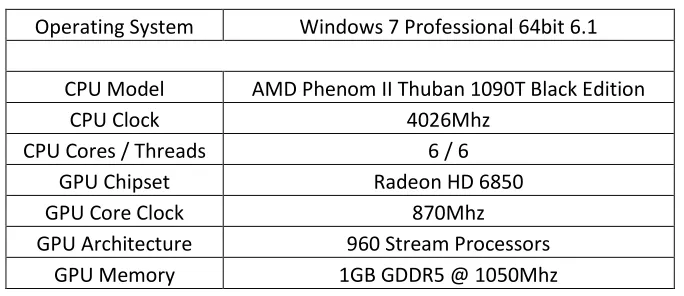
The first test bed is a powerful desktop workstation, described in Table 1. The second test

bed is a GPGPU (general purpose graphics processing unit) laboratory desktop computer,

shown in Table 2. The third test bed is a rack-mount server, shown in Table 3. The final

test bed is an older laptop computer, included to show the relative performance of a

legacy machine. The specifications for this test bed are shown in Table 4.

Table 1: Workstation desktop test bed specifications.

Operating System Windows 7 Professional 64bit 6.1

CPU Model AMD Phenom II Thuban 1090T Black Edition

CPU Clock 4026Mhz

CPU Cores / Threads 6 / 6

GPU Chipset Radeon HD 6850

GPU Core Clock 870Mhz

GPU Architecture 960 Stream Processors

(44)

Table 2: Laboratory desktop test bed specifications.

Operating System Ubuntu 64bit 3.8.0

CPU Model Intel Xeon E5504, Intel Xeon E5504

CPU Clock 1596Mhz

GPU Chipset nVIDIA Tesla c2070

GPU Core Clock 1150Mhz

GPU Architecture 448 Stream Processors

GPU Memory 6GB GDDR5 @ 1500Mhz

Table 3: Rack-mount server test bed specifications.

Operating System GNU Linux 64bit 2.6.32

CPU Model Intel Xeon E5603

CPU Clock 1197Mhz

Table 4: Legacy laptop test bed specifications.

Operating System Windows 7 Professional 64bit 6.1

CPU Model AMD Turion x2 TL-56

CPU Clock 1800Mhz

4.3 Python

The results of comparing the performance of a Python implementation of the serialSinc

algorithm across the four test bed hardware platforms described above are shown in

Figure 10. The raw data for this comparison are provided in Appendix C. Each running

time presented is the mean of 5 trials of executing the algorithm. Because of the three

nested FOR loops used to iterate through the voxels in a sinc kernel, as the size of sinc

kernel along the three dimensions increases the running time increases as a cubic

(45)

Figure 10: Python implementation running time comparison across test beds.

This performance comparison shows several interesting differences between the four test

beds when using a sinc kernel of size 7 x 7 x 7. Firstly, one might expect that the two

Intel processors, being of similar model numbers and specifications, would have similar

performance with the legacy laptop lagging behind. Instead, the AMD Turion TL-56 and

the Intel E5603 perform quite similarly at 13147 seconds and 13647 seconds

respectively, however still with a significant difference in performance between them

(F(2,5) = 15700, p < 0.000001). These two processors both execute the algorithm much

more slowly than the Intel Xeon E5504 at 9069 seconds (F(2,5) = 6888131, p <

0.000001). Also notice that the AMD Turion TL-56, despite its faster clock speed, does

not outperform the Intel Xeon E5504. This gap in performance could be explained by

AMD Turion TL-56's small cache compared to the Intel Xeon E5504: 1024KB L2 cache

versus 4096KB L2 cache respectively. The AMD Thuban 1090T, with a high clock speed

and advanced architecture, outperforms the next fastest processor with a running time of

(46)

Importantly, regardless of the test bed hardware platform, the Python implementation of

the 3D sinc interpolation algorithm was not able to interpolate the voxel intensities for an

entire fMRI time series with a sinc kernel size of 13 x 13 x 13 within a tractable length of

time. Extrapolating based on the performance of the fastest hardware platform, the AMD

Thuban 1090T, it would take an estimated 21195 seconds or 5.9 hours to complete the

interpolation of one volume; extrapolating based on the performance of the slowest

hardware platform, the Intel Xeon 5603, it would take an estimated 60577 seconds or

16.8 hours to interpolate one volume. This means that at best, a Python implementation

of the serialSinc algorithm could interpolate the data from an example 800 volume scan

(20 minutes, TR = 1.5 seconds) in slightly over 6 months; surely an intractable length of

time.

Performance Comparison of 3D Sinc Interpolation for fMRI Motion Correction by Language of Implementation and Hardware Platform

Scholarship@Western

Scholarship@Western

Performance Comparison of 3D Sinc Interpolation for fMRI

Performance Comparison of 3D Sinc Interpolation for fMRI

Motion Correction by Language of Implementation and Hardware

Motion Correction by Language of Implementation and Hardware

Platform

Platform

Abstract

Keywords

Acknowledgments

Table of Contents

List of Tables

List of Figures

List of Appendices

Preface

Chapter 1

1

Functional Magnetic Resonance Imaging

1.1 Magnetic Resonance Imaging Physics

1.2 fMRI Motion Correction: Overview

1.3 fMRI Motion Correction: General Algorithm

Chapter 2

2

Interpolation Methods in fMRI Motion Correction

2.1 Trilinear Interpolation

2.1.1

Algorithm

2.1.2

AIR Software Package

2.2 Spline Interpolation

2.2.1

Algorithm

2.2.2

SPM2 Software Package

2.3 Fourier Interpolation

2.3.1

Algorithm

2.3.2

AFNI Software Package

2.3.3

PACE Motion Correction

2.4 Sinc Interpolation

2.4.1

Algorithm

2.4.2

FSL MCFLIRT Software Package

2.5 Other Motion Correction Techniques

Chapter 3

3

Three Dimensional Sinc Interpolation

3.1 Algorithm

3.2 Serial Implementation

3.3 Parallel Implementation

Chapter 4

4

Performance Benchmarking

4.1 Experimental Setup

4.2 Test Beds

4.3 Python

4.4 C