AN ENHANCED METHOD OF LMS
PARAMETER ESTIMATION FOR
SOFTWARE REALIABILITY MODEL
Swamydoss D
1, Dr. G.M. Kadhar Nawaz
2Research Scholar, Adhiyamaan College of Engineering, Hosur,Tamilnadu, India1 Director, Dept. of MCA, Sona College of Technology, Salem, India2
Abstract: A software reliability model specifies the form of a random process that describes the behavior of software failures with respect to time. In this work the author has taken a Non Homogenous Poisson software reliability model called Gompertz model to predict the reliability of the software. It is shown that the proposed model can be derived from the well-known statistical theory of extreme value and has the quite similar sympatric property to the classical Gompertz curve. We have applied the Gompertz software reliability model to assess the software reliability and to predict the number of initial fault contents. The parameters used in this model are unknown, estimating this model parameter using an alternative approach of Least Mean Square estimation method. This new parameter estimation approach may function better than the existing estimation methods and is attractive in terms of goodness of fit, test based on information criteria and mean squared error. Software undergoes several stages of testing before it is put into operation. In every stage of testing, modification and correction are made with the hope of increasing reliability. All existing software reliability models are developed for the software products that are statically constructed normally by a company or institution that has the full control of the development process. The evolutional shift from the product-oriented software architecture to the Service Oriented Architecture (SOA) and Web Services (WS) invalids many techniques developed for traditional software. Hence in this work we have considered web based application with alternative approach for parameter estimation in Gompertz software reliability model.
Keywords: Software Reliability Model, Gompertz model, Least Mean Square Estimation, Web based Applications
I. INTRODUCTION
to assess quantitatively the software reliability which is the probability that the software system does not fail during a specified time period. Measurement of software reliability involves estimation of software reliability or its alternate quantities from failure data. The term software reliability prediction is defined by Hechtr (1977), the process of computing software reliability parameters from program characteristic. Typically, software reliability prediction takes into account factors such as the size and complexity of a program, and it is normally performed during a program phase prior to test. The principal objective of a software reliability model is to forecast failure behavior that will be experienced when the program is operational. This expected behavior changes rapidly and can be tracked during the period in which the program is tested.
II. SOFTWARE RELIABILITY ENGINEERING (SRE)
Software testing is an important process of software development to ensure the quality of software products. For large and complex system, testing becomes more complex. Although much research has advanced the techniques for generating test cases with high defect coverage, testing to guarantee defect free software remains difficult. Alternatively an empirical software reliability prediction technique is used to estimate the reliability of the software product (Rattikorn Hewetti et al 2006). The software reliability prediction is defined as the forecast of, how reliable an executable software system will be at some point in the future based on data available now. This is based on the industry definition of software reliability namely the probability of failure-free execution of a software system for a specified time in a specified operating environment. There is a difference between estimation and prediction of software reliability. The estimation is an assessment of how reliable a software system is now based on observed test data. Prediction is usually limited to a project period prior to system test. In other words, for prediction a development organization takes information about the system under development and uses some statistical regression model to forecast the level of reliability that will be present at some point in testing (Peter Lakey 2002). Reliability is probably the most important characteristics inherent from software quality. It is intimately connected with defects, it is the probability that the software without failure for a specified period of time. In addition to its preeminent importance, software reliability has proved to be the most readily quantifiable of the attributes of software reliability. Reliability is a much richer measure. It is a customer or user oriented rather than developer-oriented. Thus reliability measures are more useful than fault measures (John Musa et al 1987). As faults are removed, as in test phase, failure intensity tends to decrease and reliability increases. When faults are introduced during operation or test, as in cases when new features or design changes are being introduced into the system or when faults predominate repairs during debugging, there tends to be a step increasing in failure intensity and a step decreasing in reliability. If a system is stable, as in a program that has been released and there is no changes in code, both failure intensity and reliability tend to be constant (Dong Nguyen and Thomoson 2001). In reality, SRE tasks are fundamentally linked to both software and test engineering. SRE is just a quantitative perspective of software quality management (Koji Ohishi et al 2005 and Amrit Goel 1985).
III. SOFTWARE RELIABILITY MODELS (SRM)
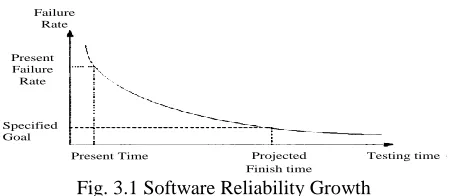
Failure Rate
Specified Goal
Present Time Projected Finish time Present
Failure Rate
Testing time
Fig. 3.1 Software Reliability Growth
Software reliability growth models are designed to make predictions. Predictions of actual reliability or failure rate time needed to reach a given reliability target and things like that. In practice, software reliability growth models encounter major challenges. First of all, software testers seldom follow the operational profile to test the software, so what is observed during software testing may not be directly extensible for operational use. Secondly, when the number of failures collected in a project is limited, it is hard to make statistically meaningful reliability predictions. Thirdly, some of the assumptions of Software reliability Growth Model (SRGM) are not realistic e.g. the assumption that the faults are independent of each other, that each fault has the same chance to be detected in one class; and that corrections of a fault never introduces new fault (Deepak Pengoria and Saurabh 2009). Vladimir Zeljkovic et al (2011),the authors have made a study on reliability and show that the software reliability cannot be calculated during the design phase. If adequate data on system failure is collected throughout the project during testing phase, the models could apply on the parameter to predict the reliability. They have also observed that the importance of reliability estimation during the testing phase.
Most reliability growth models depend on one key assumption about software system-faults are identified there by increasing the reliability of the software. The data on failures and fixes for these models is typically obtained during the final stages of testing. The growth model is used to predict the reliability of the software system at any point in time during this failure and fix process. The key issue is to obtain a good model that can explain the past data and predict the future Pankaj Jalote et al (2004 )). The SRGM falls into two categories; Time between Failure model (TBF) which treats the inter-failure interval as a random variable and Failure Count (FC) models, which treat number of failures in a given period as a random variable. In case of TBF models the parameters of inter-failure distribution change as testing proceeds, while the software reliability evolution in FC models is described by letting the parameters of distribution such as mean value function, be suitable functions of time. One of the basic assumptions common to both classes of models is that the failures, when the faults are detected are independent (Katerina Goseva 2000). The basic principle of time domain software reliability modeling is to perform curve fitting of observed time-based failure data by a pre-specified model formula, such model can be parameterized with statistical technique. The model can then provide estimation of existing reliability or prediction of failure reliability by extrapolation techniques. Estimating remaining defects in software can help test managers make release decisions during testing. Several methods exist to estimate defect content, among them a variety of software reliability models. Software reliability growth model have underlying assumptions that are often violated in practice, but empirical evidence has shown that many are quite robust despite these assumption violations. The problem is that because of assumption violations, it is often difficult to know which models to apply in practice (Stringfellow and Amschler Andrews 2002 and Bev Littlewood 1979).
IV.GOMPERTZ SOFTWARE RELIABILITY MODEL
accumulated in batches before being implemented. A good test plan is helpful, if not absolutely required, in achieving homogeneous test and debug effort. Gompertz model is also one of the S-Shaped software reliability growth model. This model will give good approximation to a cumulative number of software faults observed in testing software. The Gompertz model is an Non Homogeneous Poisson Process (NHPP) model. It takes the number of faults per unit of time as independent Poisson random variables. The model was first proposed in 1979 by Amrit Goel and Kazu okumoto and has formed the basis for the models using the observed number of faults per unit time group. Recently an enhanced model of Gompertz known as discrete Gompertz curve by discretizing the usual Gompertz equation is proposed and applies it to predict the number of defected software faults. Since the Gompertz curve is deterministic curve, one cannot access quantitatively the software reliability and its related software dependability measures. To overcome this, the NHPP model with the mean value function with Gompertz curve has been used in our work. In addition, the most severe problem is that the method of maximum likelihood cannot be easily applied to estimate the parameter in this model, because of its strong non-linearity. An alternative way for the development of an NHPP model based on the Gompertz curve is to allow a discontinuous mean value function (Dimitri Kececioglu et al 1994).
The Gompertz software reliability model can be expressed by;
µ(t) = (4.1)
Where µ(t) is the software reliability at time t and is dimensionless percent. „a‟ is a constant that provides an upper bound to µ(t), „b‟ is a constant and „c‟ is also a Gompertz constant, which provides a shape parameter to the Gompertz model equation. A relatively small value of „c‟ promulgates rapid early reliability growth while large values of „c‟ indicate slower reliability. The approach to estimate values of „a‟,‟ b‟ and „c‟ is discussed in section 5.
V. LEAST MEAN SQUARE ESTIMATION
The Least Mean Square (LMS) estimation algorithm was introduced by Widrow and Hoff in 1959 as an adaptive algorithm, which uses a gradient-based method of steepest decent. Compared to other algorithms LMS algorithm is relatively simple. It neither requires correlation function calculation nor does it require matrix inversions (Tsai et al (2004)). LMS estimation is a method for predicting or estimating the value of a single random variable „y‟ from a single measurement „x‟, when certain condition of linearity can be assumed. This method is based on the observed outcome sequence of software runs during software testing (Bo Yang et al (2008)). There are three steps in analysis;
Preliminary examination of sample data
Estimation of a regression line
Computation of confidence limits
Preliminary estimation of sample data: In a linear regression analysis one must first conduct a preliminary
examination of sample data to determine the validity of an assumption of linear dependence. Suppose that the data consist of a set
of n paired observations of measurement „x‟ and measurement „y‟, then the simplest method of examining the data is to develop a scatter diagram of the data by plotting the coordinates of n paired measurements. The scatter diagram provides a visual display of the
relationship of the data. If the points in the scatter diagram seem to fall along a line, there is an indication that values of y are on the average, linearly dependent on values of „x‟. Hence the data are appropriate.
Estimation of a Regression Line: If a preliminary examination of sample data suggests that it is reasonable to
assume a linear dependence of y on x, postulate that the mean of y is linearly related to x. Therefore, we have, E[Y] = α +βx
Where α and β are parameters to be estimated from the data. Note that α and β represent the intercept and slope of the line respectively.
The principle use of the method of LMS is to determine the best fit of a linear function to the
data . It minimizes the sum of the squares of the deviation between what we expect and
S is minimized
Differentiating S with respect to α and β,
(5.1)
(5.2)
By setting the partial derivatives equal to 0 the normal equations can be obtained. The solution of the normal equations is the Least Squares estimates.
Computation of confidence limits: Having obtained a least squares estimate of the regression line, the next step of
regression analysis is the computation of confidence limit for the intercept, slope, or regression line that are useful in evaluating the accuracy of the estimate.
The Least Mean Square algorithm is most commonly used algorithm because of its simplicity and a reasonable performance. Since it is iterative algorithm it can be used in a highly time varying testing environment (Musa and Okumo 1984).
VI. PROPOSED APPROACH OF LMS
The work aims to identify effective parameter estimation method in software reliability. In particular we have found a better estimation method using LMS algorithm. In LMS algorithm, number of defects and time interval are the two variables used to estimate the model parameters. But in software reliability number of defects are always depend on number of test cases. To effectively use the reliability models and defect data during software testing we propose to additionally apply the strategy called number of test cases for the particular module so that the number of defects are considered with respect to number of test cases. This strategy has been used in this work.
The following steps involved in estimating the Gompertz model parameters namely „a‟, „b‟ and „c‟. 1. Consider the sample data „time‟ and number of defects and number of test cases.
2. Calculate the reliability R for the available data using number of failures, number of test cases and time interval. In existing approach of LMS, reliability R is calculated only by using number of failures and time interval.
3. Calculate log R value and group the data into three equal size groups and find the sums s1, s2
and s3.
4. From s1, s2 and s3 calculate the value of „a‟ , „b‟ and‟ c‟ using the following;
(6.1)
(6.2)
(6.3)
5. Substitute the value for „a‟, „b‟ and „c‟ into Gompertz equation to obtain the value of µ(t) at point of time „t‟.
VII.MODEL EXPERIMENTATION
There are three main risks when applying software reliability growth models to estimate reliability. They are;
Not any one model will match a company‟s development and test process exactly.
Data is grouped by week resulting in a smaller amount of data.
Testing effort may vary week to week.
To handle all these risks, the approach applies several software reliability growth models cumulative failure data grouped by weeks to determine how well the method predicts the expected total number of failures.The step by step process is as follows;
Record the cumulative number of failures found in system test at the end of each week.
Determine whether enough of the test plan has been executed to contemplate when to stop testing based on applying a model. This requires setting a threshold that determines when to start applying a model to the defect data.
The curve fit program estimates a model‟s parameters by attempting to fit the model to the data.
If the model converge, it returns estimate for the expected number of total failures
Whether the reliability value is fit with the threshold value or not? If yes, concluded that the reliability value is good enough to stop the testing process.
If no model has a stable prediction for the current week, the system test continues and failure data for another week will be taken and continue the same process.
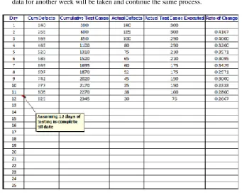
Fig. 7.1Testing result for module1 for Project Online Services
In above example, we have used current predicted defects, 825 as parameter “a” and test case efficiency of 0.27 as parameter “b”. We want to predict defects on 25th day. Using below formulas for µ(t) and CI Res, we can have
predicted 880 as overall defects with 95% confidence level and would need another 10 days of testing. Step #1: Compute µ(t), the predicted defects till date using Gompertz model
Use formula µ(t) = , a> 0, b > 0, to get predicted defects till date, where
b = the rate at which defect-rate decreases, i.e. rate at which defects are detected.
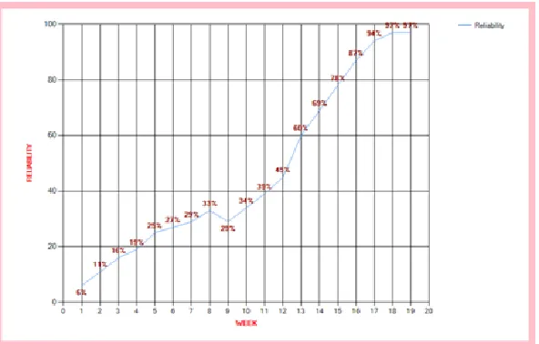
Step #2: Using this calculated reliability, the parameters of Gompertz model „a‟, „b‟ and „c‟ are calculated by using the equations 6.1,6.2 and 6.3.
Step #3: These parameters „a‟, „b‟ and „c‟ are applied on Gompertz model equation to predict the reliability of the module1 of project „Online Services‟ for 20th day, 25th day etc.
Fig. 7.2 Simulation tool to calculate Reliability and „a‟, ‟b‟ and „c‟
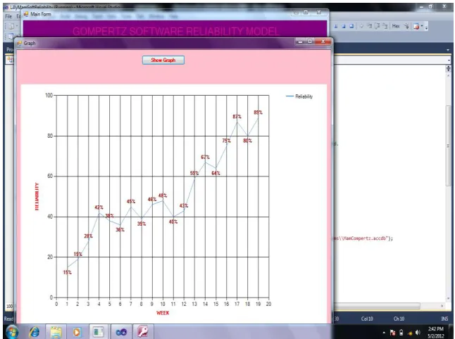
We apply the existing LMS parameter estimation method to the same data. We reached that the method use only two parameters namely, time interval and number of defects. The numbers of test cases are not considered.
Fig. 7.4 Reliability Growth Estimation using Existing LMS for module1 of Project Online Services
By comparing and observing the results obtained from these models, we could strongly convince that the proposed approach of parameter estimation gives better reliability prediction than other methods. In our approach we have taken number of test cases along with number of defects while calculating the reliability of the module. Reliability of each module can be calculated by the proposed method and hence the reliability of the project can be calculated.
VIII. CONCLUSION
This work has shown the accuracy of Gompertz software reliability model with alternative approach of parameter estimation. In particular, the test cases of each module have been taken along with number of defects. This work has proved that the proposed method is more appropriate for the testing team to make a decision about when to stop the process of testing. We proposed a three parameter estimation method based on different types of data available using Least Mean Square (LMS) estimation. In general the reliability at time„t‟ is estimated using two input values, they are; time interval and number of failures. The reliability estimation formula used in all the models is R = exp(-λt), where λt is number of failures with respect to time. In Gompertz model the reliability R is calculated using the
REFERENCES
[1]. Hecht, H. “Measurement, estimation and prediction of software Reliability”, Software Engineering technology, NASA Research Centre, Vol. 2 pp. 209-224, 1977.
[2]. Rattikorn Hewett, Remzi Seker and Catherine Stringfellow, “on Effective Use of Reliability Models and Defect Data in Software Development”, Proceedings of IEEE Conference on Software Engineering Advanced Applications, pp. 67-71, 2006.
[3]. Peter B. Lakey, “Software Reliability Prediction is not a Science ...Yet”, e-Book by Physics and Astronomy – Natural Science, 2010. [4]. John D. Musa and Anthony Iannino, Kazuhira Okumoto, “Software Reliability Measurement, Prediction, Application”, McGraw Hill,
New York, 1987.
[5]. Dong Nguyen and Thomoson, “Failure modes and Effects Analysis for Software Reliability”, Proceedings of IEEE Annual Reliability and Maintainability symposium, 2001.
[6]. Koji Ohishi, Hiroyuki Okamura and T. Dohi, “Gompertz Software Reliability Model and Its Application”, IEEE International Computer Software and Applications Conferences, Vol. 2, pp.405-410, 2005.
[7]. Michael R. Lyu and Allen Nikora, “CASRE – A Computer Aided Software Reliability Estimation Tool”, IEEE Conference on Computer Aided Software Reliability, pp.264-275, 1992.
[8]. Deepak Pengoria and Saurabh Kumar, “A Study on Software Reliability Engineering Present Paradigms and its Future Considerations”, ISSRE, 2009.
[9]. Vladimir Zeljkovi, Nela Radovanovic and Dragomir, “Software Reliability: Models and Parameters Estimation”, Scientific Technical Review, Vol. 61, No. 2 pp. 57-60, 2011.
[10]. Pankaj Jalote, Brendan Murphy, Mario Garzia and Ben Errez, “Measuring Reliability of Software Products”, Tech Report, Microsoft Research, MSR-TR-2004-145, IEEE, pp. 1-14, 2004.
[11]. Katerina Goseva, “Failure Correlation in Software Reliability Models”, IEEE Transaction on Reliability, Vol. 49, No.1, pp. 232-241, 2000.
[12]. String fellow and A. Amschler Andrews, “An Empirical Method for Selecting Software reliability growth Models”, Journal of Empirical Software Engineering, Vol. 7, No. 4, pp. 319 – 343, 2002.
[13]. Bev Littlewood, “How to Measure Software Reliability and How Not To”, IEEE Transactions on Reliability, Vol.28, No. 2, pp. 110-117, 1979.
[14]. Sulthan Aljahdali, Alaa Sheta and Muhammad Habib, “Software Reliability Analysis using Parametric and Non-parameteric Methods”, Proceeding of the ISCA 18th International Conference Computers and Their Applications (CATA), Honolulu, Hawaii, USA, 2003.