Arithmetic Cryptography

(1)

Arithmetic Cryptography

∗

Benny Applebaum† Jonathan Avron∗ Christina Brzuska‡

Tuesday 14th _{April, 2015}

Abstract

We study the possibility of computing cryptographic primitives in a fully-black-box arith-metic model over a finite fieldF. In this model, the input to a cryptographic primitive (e.g.,

encryption scheme) is given as a sequence of field elements, the honest parties are implemented by arithmetic circuits which make only a black-box use of the underlying field, and the ad-versary has a full (non-black-box) access to the field. This model captures many standard information-theoretic constructions.

We prove several positive and negative results in this model for various cryptographic tasks. On the positive side, we show that, under reasonable assumptions, computational primitives like commitment schemes, public-key encryption, oblivious transfer, and general secure two-party computation can be implemented in this model. On the negative side, we prove that garbled circuits, multiplicative-homomorphic encryption, and secure computation with low online com-plexity cannot be achieved in this model. Our results reveal a qualitative difference between the standard Boolean model and the arithmetic model, and explain, in retrospect, some of the limitations of previous constructions.

∗

A preliminary version of this paper has appeared in the 6th Innovations in Theoretical Computer Science (ITCS), 2015.

†

School of Electrical Engineering, Tel-Aviv University,{[email protected],[email protected]}. Sup-ported by ERC starting grant 639813 ERC-CLC, ISF grant 1155/11, Israel Ministry of Science and Technology grant 3-9094, GIF grant 1152/2011, and the Check Point Institute for Information Security.

‡

(2)

1 Introduction

This paper studies the possibility of solving cryptographic problems in a way which is independent from the underlying algebraic domain. We start by describing a concrete motivating example.

Consider the problem of computing over encrypted data where Alice wishes to store her private data x = (x1, . . . , xn) encrypted on a server while allowing the server to run some program f

on the data. Let us assume that each data item xi is taken from some large algebraic domain

F (e.g., finite-precision reals) and, correspondingly, the program f is described as a sequence of

arithmetic operations overF. Naturally, Alice would like to employ afully homomorphic encryption

(FHE) [Gen09]. However, standard FHE constructions typically assume that the data is represented as a binary string and the computationf is represented by a Boolean circuit.

One way to solve the problem is to translatexandf to binary form. Unfortunately, this solution suffers from several limitations. First, such a translation is typically expensive as it introduces a large overhead (typically much larger than log|_F|).1 Secondly, such an emulation is not modular as it strongly depends on the bit-representation ofx. Finally, in some scenarios Boolean emulation is simply not feasible since the parties do not have an access to the bit-wise representation of the field elements. For example, the data items (x1, . . . , xn) may be already “encrypted” under some

algebraic scheme (e.g., given at the exponent of some group generator or represented by some graded encoding scheme [GGH13]).

A better solution would be to have an FHE that supports F-operations. Striving for full

generality, we would like to have an FHE that treats the field or ring F as an oracle which can

be later instantiated with any concrete domain. In this paper we explore the feasibility of such schemes. More generally, we study the following basic question:

Which cryptographic primitives (if any) can be implemented independently of the un-derlying algebraic domain?

We formalize the above question via the following notion ofarithmetic constructions of crypto-graphic primitives.

1.1 The Model

Cryptographic constructions. Standard cryptographic constructions can be typically described by a tuple of efficient (randomized) algorithms P that implement the honest parties. The inputs to these algorithms consist of a binary stringx∈ {0,1}∗ (e.g., plaintext/ciphertext) and a security parameter 1λ which, by default, is taken to be polynomial in the length of the input x. These algorithms should satisfy some syntactic properties (e.g., “correctness”) as well as some security definition. We assume that the latter is formulated via a game between an adversary and a chal-lenger. The construction issecurefor a class of adversaries (e.g., polynomial-size Boolean circuits) if no adversary in the class can win the game with probability larger than some predefined threshold.

Arithmetic constructions. In our arithmetic model, the input x= (x1, . . . , xn) to the honest

partiesP is a vector of generic field elements. The honest parties can manipulate field elements by applying field operations (addition, subtraction, multiplication, division, and zero-testing). There

1

(5)

is no other way to access the field elements. In particular, the honest parties do not have an access to the bit representation of the inputs or even to the size ofF. We also allow the honest parties to

generate the field’s constants 0 and 1, to sample randomfield elements, and to sample randombits. Overall, honest parties can be described by efficiently computable randomizedarithmetic circuits. (See Section 3 for a formal definition.)

In contrast to the honest parties, the adversary is non-arithmetic and is captured, as usual, by some class of probabilistic Boolean circuits (e.g., uniform circuits of polynomial-size). Security should hold for any (adversarial) realization of F. Formally, the standard security game is

aug-mented with an additional preliminary step in which the adversary is allowed to specify a field by sending to the challenger a Boolean circuit which implements the field operations with respect to some (adversarially-chosen) binary representation. The game is continued as usual, where the ad-versary is now attacking the constructionPF_{. Note that once}_F_{is specified,}_PF _{can be written as a} standard Boolean circuit. Hence security in the arithmetic setting guarantees that the construction

PF _{is secure for any concrete field oracle}_F _{which is realizable by our class of adversaries.}2

Example 1.1 (One-time encryption). To illustrate the model let us define an arithmetic perfectly-secure one-time encryption scheme. Syntactically, such a scheme consists of a key-generation algorithmKGen, encryption algorithm Enc, and decryption algorithm Dec which satisfy the perfect correctness condition:

Pr

k←KGenR n

[Deck(Enck(m)) =m] = 1, for every message m∈Fn.

Perfect security can be defined via the following indistinguishability game: (1) For a security param-eter 1n, the adversary specifies a field F and a pair of messages m0, m1 ∈ Fn; (2) The challenger

responds with a ciphertext c = Enck(mb) where k R

← KGenn and b R

← {0,1}; (3) The adversary outputs a bit b0 and wins the game ifb0 =b. The scheme is perfectly-secure if no (computationally-unbounded) adversary can win the game with more than probability 1₂.

A simple generalization of the well-known one-time pad gives rise to an arithmetic one-time encryption scheme. The key generation algorithm samples a random key k ←R _Fn_{, to encrypt a} message m ∈ Fn we output m+k and to decrypt a ciphertext c ∈ Fn we output the message c−k. All the above operations can be implemented by randomized arithmetic circuits. It is not hard to see that the scheme is perfectly-secure. Namely, for any field F (or even group) chosen by

a computationally-unbounded adversary, the winning probability cannot exceed 1₂.

1.2 Our Contribution

Our goal in this paper is to find out which cryptographic primitives admit arithmetic constructions. We begin by observing that, similarly to the case of one-time pad, typical information-theoretic con-structions naturally arithmetize. Notable examples include various secret sharing schemes [Sha79, DF91, CF02], and classical information-theoretic secure multiparty protocols [BOGW88, CCD88].

2

(6)

(See Section 1.4 for a detailed account of related works.) This raises the natural question of con-structing computationally secure primitives in the arithmetic model. We give an affirmative answer to this question by providing arithmetic constructions of several computational primitives.

Informal Theorem 1.1. There are arithmetic constructions of public-key encryption, commitment scheme, oblivious linear evaluation (the arithmetic analog of oblivious transfer), and protocols for general secure multiparty computation without honest majority (e.g., two-party computation), as-suming intractability assumptions related to linear codes.

We emphasize that our focus here is on feasibility rather than efficiency, and so we did not attempt to optimize the complexity of the constructions. The underlying intractability assumption essentially assumes the pseudorandomness of a matrix-vector pair (M,y˜) where M is a random

m×n generating matrix and ˜y∈_Fm _{is obtained by choosing a random codeword}_y_∈_colSpan(_M₎

and replacing a random p-fraction of y’s coordinates with random field elements.3 This Random-Linear-Code assumption, which is denoted byRLC_F(n, m, p), was previously put forward in [IPS09]. If F is instantiated with the binary field, we get the standard Learning Parity with Noise (LPN)

assumption [GKL88, BFKL93]. Indeed, some of the primitives in the above theorem can be con-structed by extending various LPN-based schemes from the literature. (See Section 2.2.)

Theorem 1.1 shows that the arithmetic model is rich enough to allow highly non-trivial compu-tational cryptography such as general secure two-party protocols. As a result, one may further hope to arithmetize all Boolean primitives. Our main results show that this is impossible. That is, we show that there are several cryptographic tasks which can be achieved in the standard model but cannot be implemented arithmetically. This include garbled circuits, secure computation protocols with “low” online communication, and multiplicative homomorphic encryption schemes. Details follow.

Garbled circuits. Yao’s garbled circuit (GC) construction [Yao86] maps any boolean circuit

C : {0,1}n _{→ {}₀_,₁_}m _{together with secret randomness into a “garbled circuit” ˆ}_C _{along with} _n

“key” functions Ki :{0,1} → {0,1}k such that, for any (unknown) input x, the garbled circuit ˆC

together with thenkeysKx= (K1(x1), . . . , Kn(xn)) revealC(x) but give no additional information

about x. The latter requirement is formalized by requiring the existence of an efficient decoder

which recovers C(x) from ( ˆC, Kx) and an efficient simulator which, given C(x), samples from a

distribution which is computationally indistinguishable from ( ˆC, Kx). The keys are short in the

sense that their length, k, depends only in the security parameter and does not grow with the input length or the size of C. Yao’s celebrated result shows that such a transformation can be based on the existence of any pseudorandom generator [BM82, Yao82], or equivalently a one-way function [HILL99].

The definition of arithmetic garbled circuits naturally generalizes the Boolean setting. The target function C : Fn → Fm is now a formal polynomial (represented by an arithmetic circuit),

and we would like to encode it into a garbled circuit ˆC, along with n arithmetic key functions

Ki : F → Fk, such that ˆC together with the n outputs Ki(xi) reveal C(x) and no additional

information about x. As in the Boolean case, we require the existence of an arithmetic decoder

3

This is contrasted with the more standard Learning-With-Errors (LWE) assumption [Reg05] in whicheach coor-dinate ofyis perturbed with some “small” element from the ringZp, e.g., drawn from the interval±α·p. Note that

(7)

and simulator. We say that the garbling is short if the key-length depends only in the security parameter (i.e., can be taken to be nε _{for an arbitrary} _{ε >} _{0). A more relaxed notion is} _online efficiency, meaning that the key-length should be independent of the circuit complexity of C but may grow with the input length. (The latter requirement is typically viewed as part of the definition of garbling schemes, cf. [BHR12].)

The question of garbling arithmetic circuits has been open for a long time, and only recently some partial progress has been made [AIK11]. Still, so far there has been no fully arithmetic construction in which both the encoder and the decoder make a black-box use of F. The next

theorem shows that this is inherently impossible answering an open question from [Ish12].

Informal Theorem 1.2. There are no short arithmetic garbled circuits. Furthermore, assuming the existence of (standard) one-way functions, even online efficient arithmetic garbled circuits do not exist.4

Recall that in the Boolean setting short garbled circuits can be constructed based on any one-way function, hence, Theorem 1.2 “separates” the Arithmetic model from the Boolean model. The proof of the theorem appears in Section 5.

Secure computation with low online complexity. Generalizing the above result, we prove a non-trivial lower-bound on the online communication complexity of semi-honest secure computa-tion protocols. Roughly speaking, we allow the parties to exchange all the messages which solely depend on internal randomness at an “offline phase”, and then move to an “online phase” in which the parties receive their inputs and may exchange messages based on their inputs (as well as their current view). Such an online/offline model was studied in several works [Bea95, IPS08, BDOZ11, DPSZ12, IKM+13]. In the standard Boolean setting, there are protocols which achieve highly efficient online communication complexity. For example, for efficient deterministic two-party func-tionalities f :{0,1}n_{× {}₀_,₁_}n_{→ {}₀_,₁_}m _{which deliver the output to one of the parties (hereafter}

referred to as simple functionalities), one can obtain semi-honest protocols with online commu-nication of n1+ε based on Yao’s garbled circuit, or even n+o(n) based on the succinct garbled circuit of [AIKW13]. In contrast, we show that in the arithmetic model the online communication complexity must grow with the complexity of the function.

Informal Theorem 1.3. Assume that arithmetic pseudorandom generators exist. Then, for every constantc >0there exists a simple arithmetic two-party functionalityf :Fn×Fn→Fnc which

can-not be securely computed by an arithmetic semi-honest protocol with online communication smaller than Ω(nc) field elements.

The existence of an arithmetic pseudorandom generator follows from theRLCassumption. The the-orem generalizes to the multiparty setting including the case of honest majority. (See Section 6.)

Multiplicative homomorphic encryption. A multiplicative homomorphic encryption scheme is a standard public-key encryption scheme in which, given only the public key, one can transform a ciphertext c =Encpk(x) and a scalara∈F (given in the clear) into a fresh encryption c0 of the

4

(8)

producta·x. Formally, we require an efficient (randomized) transformationT such that, for every messagesx, a∈_Fand almost all public keys pk, the distributions

(c=Encpk(x), c0=T(pk, c, a)) and (c=Encpk(x), c00=Encpk(a·x)) (1)

are statistically close. Two well known examples for such schemes (over different fields) are Goldwasser-Micali cryptosystem [GM84] and ElGamal cryptosystem [ElG84].

In Section 7 we show that multiplicative homomorphic encryption cannot be implemented arith-metically.5

Informal Theorem 1.4. There are no multiplicative homomorphic encryption schemes.

In fact, the theorem holds even when the distributions in Eq. (1) are within small constant statistical distance (e.g., 1/6). Moreover, the theorem extends to the case of one-time secure private-key encryption schemes (and, under some additional conditions, to non-interactive perfectly bindingcommitments with multiplicative homomorphism). Interestingly, we can construct, in the arithmetic setting, (one-time secure) private-key encryption schemes which enjoyweak multiplicative homomorphism. Namely, only the marginals c0 and c00, defined in (1), are identically distributed. So the main issue seems to bestrong homomorphism, which cannot be achieved arithmetically, but can be easily achieved (for scalar multiplication) in the Boolean setting.

1.3 Discussion and Open Questions

Taken together, our positive and negative results suggest that the arithmetic model is highly non-trivial yet significantly weaker from the standard model. Beyond the natural interest in arithmetic constructions, our negative results explain, in retrospect, some of the limitations of previous results. For example, [AIK11] show that arithmetic garbled circuits can be constructed based on a special “key-shrinking” gadget, which can be viewed as a symmetric encryption overF with some

homomorphic properties. They also provide an implementation of this gadget over the integers. This allows to garble circuits over the ringZp in a “semi-arithmetic” model, in which the encoder

can treat the inputs as integers and the decoder is non-arithmetic. Theorem 1.2 shows that these limitations are inherent. Specifically, we can conclude that there are no arithmetic constructions of the key-shrinking gadget. Similarly, Theorem 1.3 partially explains the high online communication complexity of arithmetic MPC protocols such as the ones from [BOGW88, CCD88, CFIK03, IPS09]. Moreover, we believe that our results have interesting implications regarding the standard

Boolean model. Inspired by computational complexity theory [BGS75, RR94, AW08], one can view our negative results as some form of a barrier.

The Arithmetization Barrier: If your construction “arithmetizes” then it faces the lower-bounds.

LPN/RLC vs. LWE. As an example, it seems that constructions which are based on the Learning-Parity-with-Noise assumption typically extend to the arithmetic setting under the RLC assumption. Therefore, “natural” LPN-based constructions are deemed to face our lower-bounds. Specifically, Theorem 1.4 suggests that it may be hard to design an LPN-based encryption with

5_{In the conference version of this paper, we stated a weaker impossibility result which applied only to restricted}

(9)

(strong) multiplicative homomorphism. Since such schemes can be easily constructed under Regev’s Learning-With-Errors (LWE) assumption [Reg05], this exposes a qualitative difference between the two assumptions. Indeed, this gap between strong LWE-type homomorphism (as in Eq. 1) which can be applied repeatedly, and weak LPN-type homomorphism which can be applied only a small number of times, seems to be crucial. This gap may also explain why LWE has so many powerful applications (e.g., fully homomorphic encryption [BV11]), while LPN is restricted to very basic primitives. The weak homomorphism supplied by typical LPN-based schemes was probably noticed by several researchers. The new insight, supplied by our arithmetic lower-bound, is that the lack of strong homomorphism is not just a limitation of a concrete construction, but it is, in fact, inherent to all arithmetic constructions. Quoting Pietrzak [Pie12] one may wonder: “. . . is there a fundamental reason why the more general LWE problem allows for such (rich cryptographic) objects, but LPN does not?” A simple answer would be: “LPN arithmetize but LWE doesn’t.”

IT constructions. Another example, for which the arithmetization barrier kicks in, is the case of information-theoretic (IT) constructions. Most of the standard techniques in this domain (e.g., polynomial-based error correcting codes) arithmetize, and so these constructions are deemed to be restricted by our lower-bounds. We mention that, in the area of IT-secure primitives, proving lower-bounds (even non-constructively) is notoriously hard.6 The arithmetic model restricts the honest parties, and as a result makes lower-bounds much more accessible while still capturing most existing schemes. We therefore view the arithmetic setting as a new promising starting point for proving lower-bounds for information-theoretic primitives.

From a more constructive perspective, instead of thinking of arithmetic lower-bounds as barriers, we may view them as road signs saying that in order to achieve some goals (e.g., basing homomorphic encryption on LPN), one must take a non-arithmetic route.

Open questions. We conclude with some open questions. First, there are several basic primi-tives whose existence in the arithmetic setting remains wide open. This includes Pseudorandom Functions, Collision Resistant Hash Functions, Message Authentication Codes, and Signatures. It will be also interesting to extend our positive results to a more restricted model which does not allow to sample random bits or to apply zero-testing. In fact, in this model we do not even know how to construct a one-way function based on a “standard assumption”. On the negative side, one may ask whether our lower-bounds hold in a more liberal arithmetic model in which the parties are allowed to learn an upper-bound on the field size or to view a random representation of the field elements. (Such a model was considered by [IPS09], see Section 1.4.)

1.4 Previous Work

As already mentioned many information-theoretic primitives admit an arithmetic implementa-tion. Notable examples include one-time MACs based on affine functions, Shamir’s secret-sharing scheme [Sha79], the classical information-theoretic secure multiparty protocols of [BOGW88, CCD88] and the randomized encodings of [IK00]. Extensions of these results to generic black-boxrings were given in [DF91, CF02, CFIK03].

6_{A classical example is the share size of secret-sharing schemes for general access structure. The situation becomes}

(10)

Much less is known for computationally secure primitives. To the best of our knowledge, previous works only considered arithmetic models in which the honest parties havericher interface with the underlying field. (See below.) Therefore the resulting constructions do not satisfy our arithmetic notion.

The IPS model. Most relevant to our work is the model suggested by Ishai, Prabhakaran and Sahai [IPS09] (hereafter referred to as the IPS model) in the context of secure multiparty com-putation. In this model the parties are allowed to access the bit-representation of field elements, where the field and its representation are chosen by the adversary. This allows the honest parties to learn an upper-bound on the field size, and to feed field elements into a standard (Boolean) cryptographic scheme (e.g., encryption, or oblivious transfer). In contrast, such operations cannot be applied in our model.7 The work of Naor and Pinkas [NP99] yields semi-honest secure two-party protocols in the IPS model based on the pseudorandomness of noisy Reed-Solomon codewords. Ishai et al. [IPS09] extend this to the malicious model and to the case of general rings, and improve the efficiency and the underlying intractability assumptions. Both works rely on the existence of a Boolean Oblivious Transfer primitive.

Arithmetic reductions. Another line of works provides arithmetic constructions of high-level primitives P (e.g., secure computation protocol) by making use of a lower-level primitive Q (e.g., arithmetic oblivious-transfer) which is defined with respect to the field F. This can be viewed as

an arithmetic reduction from P to Q. Arithmetic reductions from secure multiparty computation to Threshold Additive Homomorphic Encryption were given by [FH93] for the semi-honest model, and were extended by [CDN01] to the malicious model (assuming that the underlying encryption is equipped with special-purpose zero-knowledge protocols). Similarly, the results of [AIK11] can be viewed as an arithmetic reduction from garbling arithmetic circuits to the design of a special symmetric encryption overF.

The Generic Group Model. It is instructive to compare our arithmetic model to the Generic Group Model (GGM) and its extensions [Sho97, MW98, Mau05, AM09]. The generic group model is an idealized model, where the adversary’s computation is independent of the representation of the underlying cryptographic group (or ring). In contrast, in our model the honest players are arithmetic (independent of the field), while the adversary is non-arithmetic and has the power to specify the field and its representation. Correspondingly, these two models serve very different purposes: The GGM allows to prove unconditional hardness results against “generic attacks”, while our model allows to increase the usability of cryptographic constructions by making them “field independent”. Perhaps the best way to demonstrate the difference between the models is to see what happens when the ideal oracle is instantiated with a concrete field or ring. In our model, the resulting Boolean construction will remain secure by definition, whereas in the GGM the resulting scheme may become completely insecure [Den02].

7

For example, in the IPS model a party can trivially commit to a field element x ∈ F by applying a binary

(11)

2 Techniques

2.1 Negative Results

At a high level, our main (negative) results are obtained by reducing the task of attacking arithmetic primitives to the task of “analyzing” arithmetic circuits. We solve the latter problem by making a novel use of tools (most notably partial derivatives) that were originally developed in the context of arithmetic complexity theory. Overall, our lower-bounds show that algorithms for arithmetic circuits can be used to attack arithmetic constructions. Below we give an outline of the proofs of the main negative results.

For ease of presentation, we sketch (in Section 2.1.1) a version of Theorems 1.2 and 1.3 in the Private Simultaneous Messages (PSM) model of [FKN94], which is conceptually simpler than garbled circuits and general secure computation protocols. Section 2.1.2 contains an overview of the proof of Theorem 1.4.

2.1.1 Communication Lower Bounds in the PSM model

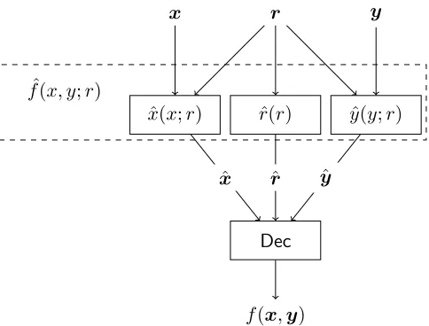
The PSM model. Consider two parties Alice and Bob that have private inputsxandy, respec-tively, and a shared random stringr. Alice and Bob are each allowed to send a single message to a third party Carol, from which Carol is to learn the value off(x, y) for some predefined function f, but nothing else. The goal is to minimize the communication complexity. In the standard (Boolean) setting, one can use garbled circuits to obtain a protocol in which Alice’s communication depends only on her input length and the security parameter k, and is independent of Bob’s input length or the complexity of f. Specifically, under standard cryptographic assumptions, Alice’s message

A(x;r) can be of length|x| ·k [FKN94], or even|x|+k [AIKW13]. In contrast, we will prove that, in the arithmetic model, the length of Alice’s message A(x;r) must grow with Bob’s input.

Let Alice’s inputx∈Fbe a single field element, let Bob’s inputyconsist of two column vectors y1, y2 ∈Fn, and letf(x,(y1, y2)) =x·y1+y2 be the target function. We will show that if Alice’s message is shorter than n, Carol can learn some non-trivial information about Bob’s input. In patricular, Carol will output a non-zero vector which is orthogonal to y1. (This clearly violates privacy as it allows Carol to exclude all but a 1/|_F|fraction of all possible inputs for Bob.) Let us assume, for now, that the parties do not use division or zero-testing gates, and so all the parties are simply polynomials over F.

We begin with a few observations. Fix the shared randomness r, Bob’s input y, and Bob’s message b =B(y;r), and consider the residual polynomials of Alice and Carol.8 Alice computes a vector of univariate polynomials Ar(x) :F → Fn−1 which takes her input x ∈F and outputs a

message a∈ _Fn−1_{, and Carol computes a vector of multivariate polynomials} _C

b(a) : Fn−1 → Fn

which maps Alice’s message a ∈_Fn−1 _{to a vector of field elements} _z_∈

Fn. By the correctness of

the protocol, we have that

fy1,y2(x) =Cb(Ar(x)), for everyx∈F, (2)

wherefy1,y2(x) =x·y1+y2. Let us fix a fieldF whose characteristic is larger than the degree of

the polynomial Cb(Ar(x)).9 Over such a large field, the univariate polynomial in the RHS of (2)

8

We use bold fonts for fixed value, and standard fonts for non-fixed values which are treated as formal variables.

9_{Since the polynomial}_C

b(Ar(x)) can be computed by a circuit of sizes= poly(n), its degree is at most 2s and

(12)

and the univariate polynomial in the LHS areformally equivalent, namely, they represent the same polynomial in F[X]. As a result, their formal partial derivatives are also equivalent:

∂fy1,y2(x)≡∂Cb(Ar(x)). (3)

By the definition off the LHS simplifies toy1, and by applying the chain rule to the RHS we get

y1 ≡ JCb(Ar(x))·∂Ar(x). (4)

Syntactically, ∂Ar(x) is a (column) vector ofn−1 univariate polynomials that contains, for each output of Ar(x) : F → Fn−1, the derivative with respect to the formal variable x. Similarly, the

Jacobian matrixJCb(a) :Fn−1 →Fn×n−1 is a matrix of multivariate polynomials whose (i, j)-th

entry is the partial derivative of the i-th output of Cb(a) : Fn−1 → Fn with respect to the j-th

input (the formal variableaj).

Let us now get back to Carol’s attack. Carol does not knowrand therefore she cannot compute neitherAr(x) nor its derivative∂Ar(x). However, she knowsband therefore can compute a circuit for Cb, which, by using standard techniques, can be transformed into a circuit for the Jacobian JCb. Carol also received from Alice a message a=Ar(x), wherex is Alice’s input, and so Carol can evaluate the circuitJCb at the pointaand obtain the matrixM=JCb(a)∈Fn×(n−1). Now,

the key observation is that

y1=M·v, for some (unknown) vectorv.

Indeed, this follows by evaluating the RHS of (4) at the pointx(and takingv=∂Ar(x)). Overall, Carol now holds a matrix M whose columns span Bob’s input y1 ∈ Fn. Since M has only n−1

columns, Carol can find a non-zero vector which is orthogonal to y1 and break the security of the protocol.

Handling zero-test gates. If the parties use zero-test gates then the functions computed by Alice and Carol are not polynomials anymore. As a result, (3) does not hold since the partial derivative of the function P(x) =Cb(Ar(x)) is not defined. To solve the problem we show that it is possible to remove the zero-test gates. Assume, for simplicity, that the circuit P(x) contains a single zero-test gate which is applied to the expression Q(x). Note that Q(x) is a polynomial of degree dwhich is much smaller than the field. We distinguish between two cases: If Q is the zero polynomial we remove the gate and replace its outcome with the constant 0; otherwise, we replace the gate with the constant 1. This transformation changes the value ofP on at mostdpoints (the roots ofQ), and therefore, the resulting polynomialP0 agrees with the polynomialfy1,y2 on all but d points. Since both functions are low degree polynomials we conclude that they must be equal. The above argument easily generalizes to a large number of zero-test gates.

Some technicality arises due to the fact that the attacker Carol does not have an access to

(13)

Extensions. The above argument shows that Alice’s communication grows with the length of Bob’s input. A stronger result would say that Alice’s communication grows with the complexity of the function (even if Bob’s input is also short). We can prove such a result via the use of a pseudorandom generator (PRG). Roughly speaking, we embed a PRG in the function f such that a low communication protocol allows to break the pseudorandomness of the PRG. This approach extends to the setting of arithmetic garbled circuits and general secure multiparty protocols yielding Theorems 1.2 and 1.3.

2.1.2 Impossibility of Multiplicative Homomorphic Encryption

Theorem 1.4 strongly relies on the existence of efficient algorithm for the following promise problem, denoted Arithmetic Predictability (AP): Given a pair of arithmetic circuits P : Fn → Fm and T :Fn→F distinguish between the case where

• (Predictable) For a randomly chosen x←R _Fn_{, the random variable} _T₍_x_{) is predictable given}

P(x), i.e., there exits an efficient10 predictor which given P(x) can guess, with high proba-bility, the value ofT(x); and

• (Unpredictable) For a randomly chosen x←R _Fn_{, the random variable} _T₍_x_{) is}

(information-theoretically) unpredictable given P(x), i.e., any (computationally unbounded) predictor which gets to seeP(x), fails, with high probability, to guess the value ofT(x).

To prove Theorem 1.4 we show that attacking multiplicative homomorphic encryption reduces to solving AP. The idea is simple: given a public-key pk and a ciphertext c = Encpk(b) of an

unknown plaintext b ∈ {0,1}, we use the multiplicative homomorphism to construct the circuit

P(a) = fc,pk(a) which maps a plaintext a ∈ F into a fresh encryption of a·b. Consider the

probability distribution ofP(a) induced by a uniform choice ofa←R Fand the internal randomness

of the homomorphic evaluator (herecandpkare viewed as fixed constants). Ifcis an encryption of 0 thenP(a) is simply a fresh encryption of the zero element, andP loses all information regarding a. As a result, a is unpredictable given P(a). In contrast, if c is an encryption of 1 then P(a) is a fresh encryption of a, and so, a can be predicted given P(a) (e.g., by using the decryption algorithm). Hence, an efficient algorithm for predictability allows us to break the security of the multiplicative homomorphic encryption.

Building on the techniques of Dvir et al. [DGW07], we design an algorithm that solvesAPin the case where the underlying field F is sufficiently large and the circuits (P, T) compute polynomials

(i.e., do not use division gates, zero-testing gates, and random bits). In fact, the algorithm in this case is surprisingly simple: Choose a random point x←R _Fn _{and check if the rows of the Jacobian} JP(x)∈Fm×nspan the gradient∂T(x)∈Fnof the target polynomialT(x). We further show that

the case of a generalized arithmetic circuit P with division gates, zero-testing gates, and random bits, reduces to the case where the circuit P : Fn → Fm computes polynomials. (The reduction

introduces some “error terms” which force us to consider a more robust form of AP. Fortunately, the above algorithm generalizes to this setting as well. See Section 7.)

(14)

2.2 Positive Results

Our positive results (Theorem 1.1) are based on three different approaches – outlined below.

2.2.1 Arithmetic/Binary Symmetric Encryption

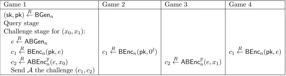
One main approach is based on a new abstract notion of arithmetic/binary symmetric encryption

(ABE). An ABE is an arithmetic symmetric encryption scheme which allows to encrypt a field element using a binary key. That is, while the scheme works in the arithmetic model, the key is essentially a string of bits given as a sequence of 0-1 field elements. Such an encryption scheme allows us to import binary constructions to the arithmetic setting, and can be therefore viewed as a bridge between the binary world to the arithmetic world.

Given, for example, a standardbinary public-key encryption scheme we obtain a newarithmetic

public-key encryption by working in a hybrid mode. Namely, to encrypt a message x∈_F, encrypt

xvia the ABE under a fresh private binary keyk, and then use the binary public-key encryption to encrypt the binary message k. Conveniently, for this purpose it suffices to have aone-time secure ABE.11

Similarly to the case of public-key encryption, ABE can be used to obtain arithmetic con-structions of CPA-secure symmetric-key encryption, and commitment schemes. In order to achieve arithmetic secure computation protocols, we will need an additional “weak homomorphism prop-erty”: Given a ciphertextEk(x) and field elementsa, b∈F, it should be possible to generate a new

ciphertext c0 which decrypts toax+b. (The new ciphertext c0 does not have to look like a fresh ciphertext – hence the term “weak homomorphism” – and so this does not contradict our negative results.) For technical reasons, we also require a “simple” decryption algorithm (e.g., one that can be implemented by a polynomial-size arithmetic formula or branching program).

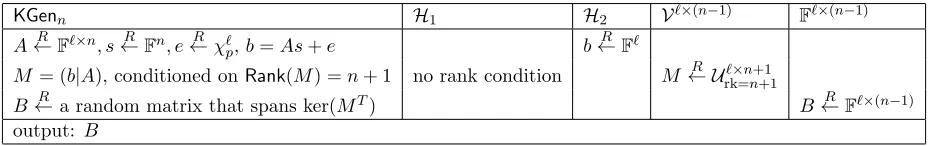
ABE based on RLC. We show that such a one-time secure ABE can be obtained under the (generalized) Random Linear Code assumption RLC_F(n, m, p). To encrypt a message x, sample

a random generating matrix A ←R _Fm×n _{together with a random} _p_{-noisy codeword} _y_{, encode the}

messagexvia a repetition code, and use the noisy codewordy to mask the encoded messagex·1m.

The resulting ciphertext consists of the pair (A, y+x·1m). The private-key is the set of all noisy

coordinates, described as a binary vector. Decryption can be implemented by ignoring the noisy coordinates and solving a set of linear equations over F. For properly chosen constants m/n and p, the system will have a unique solution, with all but negligible probability.

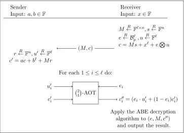
From ABE to secure computation. Let us explain how to construct secure arithmetic two-party computation from an ABE with weak homomorphism. The construction can be viewed as a variant of the construction of [IPS09]. Recall that a (binary) one-out-of-two oblivious transfer ( 2₁-OT) is a two-party functionality which takes two inputs a0, a1 ∈ {0,1}n from a sender, and a selection bit x∈ {0,1} from the receiver and delivers to the receiver the valueax.

We begin by converting a maliciously-secure binary 2₁-OT into a maliciously-secure 2₁ arith-metic oblivious transfer ( 2₁-AOT) in which the sender’s inputs a0, a1 ∈F are two field elements.

The transformation uses an ABE in the natural way: The sender encrypts the arithmetic messages

11

(15)

a0 anda1 under binary keysk0, k1, and sends the ciphertexts to the receiver; then the receiver uses the binary 2₁

-OT to select one of two keys k0, k1.

Next, we convert 2₁-AOT to Oblivious Linear Evaluation (OLE). The latter functionality takes two field elements a, b∈ _F from a sender, and another field element x ∈_F from the receiver and delivers to the receiver the value ax+b. The construction makes use of the ABE again, this time exploiting the weak homomorphism. Specifically, the receiver sends the ciphertext c=Ek(x), and

the sender uses the homomorphism to generate a ciphertext c0 which decrypts to ax+b. This ciphertext cannot be sent back to the receiver as it leaks information onaandb. Instead, a secure two-party computation protocol for decrypting c0 is invoked. Since the input of the receiver is binary (and decryption has low-complexity), such a protocol can be implemented efficiently via a

2 1

-AOT (e.g., via the protocols of [CFIK03]).12 This gives a semi-honest OLE.

At this point, we can use the semi-honest OLE together with an arithmetic variant of the classical GMW protocol [GMW87] to obtain an arithmetic secure computation protocol for general arithmetic functions in the semi-honest model. This protocol can be transformed to the malicious setting using the IPS compiler [IPS08]. To make the compiler work in our arithmetic setting, we need two additional tools: arithmetic multiparty protocol with security against a constant fraction of malicious parties (which can be constructed based on [BOGW88] or [CFIK03]), and a maliciously-secure 2₁

-AOT (which we already constructed).

2.2.2 Alternative approaches

Let us briefly mention two alternative approaches that can be used to derive arithmetic construc-tions for some of the primitives mentioned in Theorem 1.1.

Arithmetizing LPN-based scheme. As already mentioned, existing LPN-based schemes easily extend to the arithmetic setting under the (generalized) Random Linear Code assumption. This gives alternative arithmetic constructions for primitives like symmetric encryption [GRS08], com-mitments [AIK10, KPC+11], and even public-key encryption [Ale03] and 2₁

-AOT. This “direct approach” is inferior to the first (ABE-based) approach in terms of the strength of the underlying assumption. For example, using the direct approach, in order to obtain an arithmetic public-key en-cryption, we have to assumeRLC(n, m, p) for constant-rate codem=O(n) and sub-constant noise rate p=O(1/√n). In the case of CPA-secure symmetric encryption, the direct approach requires hardness forany polynomialm=m(n) and constant noisep. In contrast, for both primitives, the ABE-based approach requires only hardness for constant rate codesm=O(n) and constant noise rate p. While all three assumptions are consistent with our knowledge, the third assumption is formally weaker than (i.e., implied by) the first two. Nevertheless, we also provide proofs based on the direct approach, as it is beneficial to demonstrate that known LPN-based schemes generalize to the arithmetic setting. (See discussion in Section 1.3.)

Arithmetizing Cryptographic Transformations. Another way to construct arithmetic prim-itives is to start with some concrete construction of a simple primitiveP, and then use a standard (binary) cryptographic transformation from P to a more complex primitiveQ. For this, we have to translate the binary transformation to the arithmetic setting. Indeed, in some cases, existing bi-nary transformations have a straightforward arithmetic analog. For example, we already mentioned

12

For our concrete ABE, one can directly use 2₁

(16)

that the classical GMW construction [GMW87] of semi-honest secure computation from oblivious transfer (OT) naturally extends to the arithmetic setting [IPS09]. Similarly, we show that Naor’s transform from PRGs to commitments has an arithmetic analog. This provides another arithmetic construction of commitments whose security can be reduced to the RLC assumption.

Interestingly, some binary cryptographic transforms do not seem to arithmetize. This typi-cally happens if the construction inspects some input xi ∈ {0,1} and applies different operations

depending on whether xi equals to zero or xi equals to one. This kind of arbitrary conditioning

cannot be implemented in the arithmetic setting asxi varies over a huge (possibly exponential size)

domain. As a typical example, consider the classical GGM construction [GGM86] of pseudorandom functions (PRFs) from pseudorandom generators (PRGs). In the GGM construction, the value of the PRF Fk on a point x∈ {0,1}n is computed by walking on an exponential size tree of

length-doubling PRGs, where thei-th step is chosen based on thei-th bit of the input. It is not clear how to meaningfully adopt such a walk to the arithmetic case in which xi ∈ F. Similar “conditioning

structure” appears in the Goldreich-Levin construction of hardcore predicates [GL89], and Yao’s construction of garbled circuits from one-way functions. In fact, in the latter case our negative results show that finding an arithmetic analog of the binary construction is provably impossible. The problem of proving a similar negative result for the case of PRF, or, better yet, coming up with an arithmetic construction of a PRF, is left open for future research.

Organization. Following some preliminaries (Section 3) and definitions of arithmetic crypto-graphic primitives (Section 4), the main body of this work is divided into two parts. Part I is dedicated to lower bounds, and includes a section for each primitive: Randomized Encodings (Sec-tion 5), Secure Computa(Sec-tion (Sec(Sec-tion 6) and Multiplicative Homomorphic Encryp(Sec-tion (Sec(Sec-tion 7). The positive results appear in Part II, beginning with a presentation of the Random Linear Code intractability assumption (section 8), and proceeding with a section for each primitive: Pseudo-random Generators (Section 9), Encryption Schemes (Section 10), Commitments (Section 11) and Secure Computation Protocols (Section 12).

3 Preliminaries

In this section we provide some general preliminaries. We begin with standard background on proba-bilistic notation, indistinguishability, and entropy (Section 3.1), and basic facts about polynomials, rational functions and their derivatives (Section 3.2), and proceed with somewhat non-standard definitions of efficient field representations (Section 3.3), and generalized arithmetic circuits (Sec-tion 3.4).

3.1 Probabilistic Notation, Indistinguishability, and Entropy

Statistical distance and indistinguishability. A function µ(n) is said to be negligible in n

(denoted by neg(n)) if for any polynomial functionp(n) there existsn0 ∈Nsuch thatµ(n)≤1/|p(n)|

for anyn > n0. LetP andQbe two distributions over the finite domainU, we denote the statistical distance between P and Q by ∆(P, Q) := 1₂P

x∈U|Pr[P(x)]−Pr[Q(x)]|. When ∆(P, Q) = 0 we

(17)

denote this this by Pn s

≈Qn. We say Pn and Qn are computationally indistinguishable (denoted

by Pn c

≈Qn) if for every polynomial-size family of circuits13 A={An}, it holds that

Pr

x←RPn

[An(1n, x) = 1]− Pr x←RQn

[An(1n, x) = 1]

= neg(n).

Entropy. Forp ∈(0,1) and an integer q >1 we denote by Hq(p) be the q-ary entropy function

defined asHq(p) :=−plogq(p)−(1−p) logq(1−p). Themin-entropy H∞(X) of a random variable

X distributed over a finite domain, is defined as minx∈Supp(X)log(_Pr[_X1₌_x_]). For jointly distributed random variables (X, Y), we define the predictability [DORS08] of Y given X, by Pred(Y|X) = maxAPr[A(X) =Y],where the maximum ranges over all possible (inefficient) algorithmsA. It is

not hard to verify that the best guessing strategy for A(x) is to output the heaviest element y in the conditional distribution (Y|X=x), hence,

Pred(Y|X)def= E

x←RX

max

y Pr[Y =y|X =x]

= E

x←RX

h

2−H∞(Y|X=x)i_.

A logarithmic version of predictability is captured by Average Min-Entropy [DORS08]:

˜

H∞(Y|X)

def

=−log(Pred(Y|X)).

We will need the following useful facts, which include (1) a variant of the Markov-inequality for average min-entropy, (2) the fact that applying a function to a random variable can only loose information, as well as (3) that conditioning on a random variables with λ bits output can only reduce the average min-entropy by λ.

Fact 3.1. Let W, X, Y be (possibly correlated) random variables. Then:

1. For any δ >0, it holds that

Pr

w←RW

h

˜

H∞(YW=w|XW=w)>H˜∞(Y|X, W)−log(1/δ)

i

>1−δ,

where YW=w, XW=w denote the joint distribution of (X, Y) conditioned on the event W =w. In particular, Pr

x←RX[H∞(Y|X =x)>

˜

H∞(Y|X)−log(1/δ)]>1−δ.

2. For every function g it holds that H˜∞(Y|g(X))≥ H˜∞(Y|X). Furthermore, this holds even if g is a randomized function which uses some internal random coins which are statistically independent of Y.

3. If W has at most2λ possible values, then

˜

H∞(Y|W, X)≥H˜∞((Y, W)|X)−λ≥H˜∞(Y|X)−λ.

13

(18)

Proof. By definition,

2−H˜∞(Y|(X,W))₌

E

w←RW

[2−H∞(YW=w|XW=w)_]_,

hence, by Markov’s inequality,

Pr

w←RW

[2−H∞(YW=w|XW=w)_>₂−H˜∞(Y|(X,W))_/δ_]_{< δ,}

and the first item follows by taking logarithms.

To prove the second part note that ifA predictsY given g(X) with probabilityp, then we can define A0 _{which predicts} _Y _given _X _{with probability} _p0 _≥ _p _{by letting} _A₍_x_{) =} _A₍_g₍_x_{)). Hence,}

Pred(Y|g(X))≤Pred(Y|X). Finally, the third item is proved in [DORS08, Lemma 2.2.b].

3.2 Polynomials and Rational Functions

Notation. We letF denote a finite field. For a vectorx∈Fn, we use the notation|x|to denote

the number of elements in the vectorx. Byw(x) we denote the number of non-zero elements in x. For a vector inFn where all coordinates have the same valuexwe use the notationxn. We denote

the inner product of two vectors xand yby x·y:=Pn

i=1xiyi.

We will use bold fonts to emphasize the distinction between a formal variable x and its as-signment on a point x ∈ F. A multivariate monomial M(x) in variables x = (x1, . . . , xn) over

a finite field F is defined as M(x) = axc11· · ·xcnn , where a ∈ F and ci are positive integers. A

multivariate polynomialP(x) is a sum of monomials. If P(x) is a formal polynomial innvariables

x= (x1, . . . , xn), then it induces a functionP(x) :Fn →F. A pair of polynomialsP(x) and Q(x)

are formally equivalent (denoted by P ≡ Q) if they compute the same formal polynomial, i.e., each monomial M(x) appears in P and Q with the same coefficient. Clearly, if P ≡ Q then the corresponding functions are also equal. The converse direction also holds as long as the degrees are smaller than the characteristic of the field.

A rational functionf is a quotientv(x)/u(x) of two polynomialsv(x) andu(x) whereu(x) is not the identically zero function. Note thatf is a partial function that is undefined at pointsxwhere

u(x) = 0. We say that a pair of rational functionsf(x) =f1(x)/f2(x) and g(x) =g1(x)/g2(x) are

equal (denoted f =g) if they agree on all inputs for which they are both defined. Note that this means that the polynomialsP(x) =f1(x)g2(x) andQ(x) =f2(x)g1(x) compute the same function. The functions f and g are formally equivalent (denoted by f ≡ g) if the polynomials P(x) and

Q(x) are formally equivalent.

Derivatives We now give the standard definitions of the formal derivative of multivariate poly-nomials over finite fields as well as some background, for a comprehensive treatment of derivatives over finite fields, see [SY10].

As opposed to a Euclidean space such as R, in finite fields, there is no distance measure and

(19)

polynomial. It turns out that in this setting, formal derivatives inherit many of the properties of “standard derivatives”.14

Definition 3.2 (Partial Derivative). For a finite field F and monomial M(x) = axc11· · ·xcnn with

a ∈ F and for all 1 ≤ i ≤ n, the (formal) partial derivative with respect to xi is defined as the monomial

∂xiM(x) :=cia·xc11· · ·x

ci−1

i · · ·x cn n ,

where ci refers to ci times adding up the unit element of the field F. The partial derivative of a

polynomial is defined as the sum of the derivatives of its monomials. The partial derivative of a rational function v_u(₍x_x)₎ is defined by

∂xi

v(x)

u(x)

:= u(x)∂xiv(x)−v(x)∂xiu(x) (u(x))2

Notice that the partial derivative of a polynomial (respectively rational function) is also a polynomial (respectively rational function). Forf(x) a vector of`rational functions in nvariables (f1(x), . . . , f`(x)) we denote by ∂xif(x) the column vector (∂xif1(x), . . . , ∂xif`(x))T. In line with

using normal font x for variables and bold fontx for a specific point, the notation ∂xif(x) refers

to the partial derivative of f(x) with respect toxi evaluated at the pointx.

Definition 3.3(Formal Jacobian). Forf(x) = (f1(x), . . . , f`(x))a vector of`rational functions in

nvariables over a finite fieldF, the Jacobian matrixJf(x)is the`×nmatrix of formal derivatives

[∂x1f(x), ..., ∂xnf(x)], that is, the (i, j)-th entry of Jf(x) is∂xjfi(x).

ByJf(x) we denote all partial derivatives when evaluated at the same pointx. We denote the sub-matrix that contains only the columns of the subsets⊆ {1, . . . , n} by Jsf(x). For the formal

derivative of rational functions over finite fields, the product rule and the chain rule as commonly known, apply.

Fact 3.4 (Product Rule for Rational Functions). Let f(x) and g(x) be two rational functions inn

variables over a finite field F. Then, for all1≤i≤n, it holds that

∂xi(f(x)·g(x)) =g(x)∂xif(x) +f(x)∂xig(x).

Fact 3.5(Chain Rule). Let g(x) = (g1(x), ..., gn(x))be a vector of rational functions innvariables over a finite field F, and let f(y) be a rational function in n variables over F. Then, for all

1≤i≤n, it holds that

∂xif(g(x)) =Jf(g(x))·∂xig(x)

Lemma 3.6(Schwartz-Zippel [Sch80, Zip79]). Letf(x1, . . . , xn)be a non-zero polynomial of degree at most d over a fieldF then the number of roots of f is at most d· |F|n−1 and the probability that f(x1, . . . ,xn) = 0 for random x1, . . . ,xn is smaller than _|d_F_|.

14

For example, in this case, a polynomial is constant if and only if its derivative is the all-zero function. This rule does not apply when the degree exceeds the field’s characteristic, as demonstrated by the non-zero polynomialx|F|

(20)

3.3 Efficient Field Families

Throughout the paper, we consider finite fields whose elements have an efficient representation and whose field operations are efficiently computable. We begin by defining what it means for a Boolean circuit to implement a field.

Definition 3.7 (Circuit implementation of a field). Let F be a Boolean circuit which takes as an input, an operation op ∈ {add,subtract,multiply,divide,constant,zerocheck,sample,bitsample} and up to two `bits strings (using an appropriate encoding). F is said to be a valid implementation of the finite field F, if there is an injective mapping label:F→ {0,1}m such that the following holds:

• For every command op ∈ {add,subtract,multiply,divide} and any x, y ∈ _F it holds that

F(op,label(x),label(y)) =label(x∗_Fy) where ∗_F is the corresponding field operation.

• F(constant,0`) =label(0), andF(constant,1`) =label(1).

• If a=label(0), then F(zerocheck, a) =label(1).

• If a=label(x) for x∈_F, x6= 0, then F(zerocheck, a) =label(0).

• F(sample) implements the uniform distribution over {label(x) : x∈F}.

• F(sample) implements the uniform distribution over {label(x) : x∈ {0,1}}.

Definition 3.8 (Efficient field family). A polynomial-size Boolean circuit family F ={Fn}

imple-ments a family of fields{Fn}if each circuit Fn implementsFn. In the uniform setting, we say that a PPTF implements a field ifF(1n) outputs, with all but negligible probability, a circuitFn which implements some field (as per Definition 3.7). That is, F(1n) defines a probability distribution

over finite fields.

We often speak of the family of (distributions over) fields{_F_n}and its efficient implementation

F interchangeably. Moreover, we omit the subscriptnwhen it is clear from context. As an example of an efficient field family, for each sequence of n-bit primes {pn}_n∈N, we can implement the field family {_F_n = GF(pn)} by a (non-uniform) Boolean circuit family {Fn}. The uniform definition

captures, for example, a PPT A which chooses a random n-bit prime p and outputs a circuit which implements the field GF(p). These variants correspond to the standard distinction between uniform and non-uniform adversaries. We remark that all our results are not sensitive to uniformity issues. Specifically, our negative results hold even if the adversary is uniform, while our positive results hold both in the uniform and non-uniform adversarial model (depending on the underlying assumptions).

3.4 Arithmetic Circuits

(21)

Randomized arithmetic circuits also have two special, randomized gates: The sample gate drawns elements from the underlying field F uniformly at random, and the bitsample gate draws

a uniformly random element from the set {0,1} which contains the zero and one elements of the field.

Definition 3.9 (Arithmetic Circuit). An arithmetic circuit is a directed acyclic graph. Each input gate (source) is labeled by an input variable xi, a constant1 or 0, or a randomized gate sample or

bitsample. Internal Gates are labeled by:

{add,subtract,multiply,divide,zerocheck}

For an arithmetic circuit C(x) with n input variables and m output variables any field F induces

in the natural way a (randomized) mapping CF₍_x_{) :} _Fn _→ _Fm_{. Furthermore a field}

implementa-tion F naturally induces a Boolean circuit CF(x) which implements the mapping CF₍_x₎ _{with the}

representation F. We useCF(x), CF₍_x₎ _and _C₍_x₎ _{interchangeably, when} _F _and _F _{are clear from}

context.

Throughout this work when discussing a family of circuits C = {Cn} we assume by default

polynomial time uniformity. That is, there exist a PPT Turing machine that on input 1n outputs a description ofCn.

We will occasionally consider restricted forms of arithmetic circuits that use only subset of the types of gates. Most notably, we will considerdeterministic arithmetic circuits (which do not use sample,bitsample gates), deterministic arithmetic circuits withoutzerocheck gates (which compute rational functions) and deterministic arithmetic circuits withoutzerocheck,dividegates (which com-pute polynomials). We refer to the latter (most restricted) type of circuits as strictly arithmetic circuits. The following fact states that one can efficiently compute derivatives for deterministic arithmetic circuits withoutzerocheck gates.

Fact 3.10 (Efficient Differentiation [BS83]). Let C(x) be a deterministic arithmetic circuit of size

sin nvariables without zerocheckgates, and let f(x) be the corresponding rational function. Then for all 1≤i≤n, we can construct a circuit C0(x) which evaluates the partial derivative∂xif(x) in time O(s), and constructing C0(x) from C(x) is a polynomial-time operation.

The derivative of a circuits with zerocheckgates is not well define. (In fact, such a circuit may not compute a rational function). Still, it turns out that, over large fields, such circuits can be “approximated” well by arithmetic circuitswithout zerocheckgates. Specifically, the following fact will be useful for our lower-bounds.

Proposition 3.11 (Removing zerocheck gates). Let C : Fn → Fm be deterministic arithmetic

circuit with zerocheck gates of size s which never divides by zero, and let F= GF(p) be a

prime-order field of cardinality larger than (s+ 1)2s+1. Then, there exists a deterministic arithmetic circuit D:Fn →Fm without zerocheck gates of size sand a strictly arithmetic circuit G:Fn→F

of size at mosts2 that computes a polynomial of degrees2s+1 which satisfy the following properties: 1. For every x∈_Fn _{which is not a root of} _G _{it holds that}_C₍_x_{) =}_D₍_x₎_.

2. Dis obtained from C be replacing thei-thzerocheckgate with some constant gatebi ∈ {0,1}. Furthermore, the i-thzerocheck gate of D evaluates to bi on all the inputs x∈Fn which are

(22)

3. If C computes a polynomial thenD computes a rational function which is formally equivalent to C.

4. There exists a probabilistic algorithm that given(C, p)outputs with probability1−βthe circuits

D and Gin time poly(s,logp,log(1/β)).

Proof. The circuit D is defined by repeatedly applying the following subroutine: Choose the first zerocheck gate (according to some topological order) and consider the functiong computed by its incoming wire. Ifg is the zero function replace the gate by the constant 1 (“the zero-test passes”); otherwise, replace the gate with the constant 0 (“the zero-test fails”).

Observe that the function gi considered in the i-th iteration, is computed by a zerocheck-free

circuit of size at mosts, and therefore it is a rational function of the formui/vi where the degrees

of the numerator ui and the denominator vi are bounded by 2s. Furthermore, observe that none

of the vi is identically zero, since otherwise, the original circuit C tries to divide by zero (when

it is applied to some inputs). Using standard techniques (cf. [SY10, Proof of Thm. 2.11]) we can extract a strictly arithmetic circuit of sizesthat computes ui (resp.,vi).

Call a pointx∈Fnbad if it is a root of somenon-zero ui or some (non-zero)vi, and call itgood

otherwise. Observe that D and C agree on all the good points. Moreover, the sequence of values that a good point x induces on the zerocheck gates of the original circuit C, corresponds exactly to the constants used by D to replace these gates. Letting G be the product of all the ui and vi

we derive the first two items. Furthermore, the forth item follows by checking if each of theui’s is

identically zero via the standard Polynomial Identity Testing algorithm. (E.g., by evaluatingui on

poly(log(s/β)) random points and accepting if and only if all the outcomes equal to zero.)

It is left to prove the third item. Since theui’s andvi’s are low-degree polynomials, we have, by

the Schwartz-Zippel Lemma and by a union bound, that all but as2s+1/|_F|fraction of the inputs are good. Recall that D and C can be computed by a circuit of sizes, and therefore the degrees of the polynomial C and the numerator and denominator of D =p/q are also upper-bounded by 2s. It is not hard to show that such low-degree functions which agree on so many (good) points must be formally equivalent. Indeed, if this is not the case, then the polynomial C(x)q(x)−p(x) is a non-zero polynomial of degree 2s+1 with a fraction of 1−(s2s+1/|F|) roots. Since our field is

large|_F|>(s+ 1)2s+1, this contradicts the Schwartz-Zippel Lemma.

For some of our attacks, we will need the following variant of the zerocheckremoval procedure.

Definition 3.12 (The algorithm T). The algorithm T takes as input an arithmetic circuit C :

Fn→Fm defined over a prime field F, and a point x∈Fn. The algorithm T evaluates the circuit C on the pointx, and replaces eachzerocheckgategwith the constant1or the constant0depending on the value of thatxinduces ong. At the end, it outputs the resultingzerocheck-free circuit C0(x).

Imagine that the circuit C = B ◦A consists of a composition of two arithmetic circuits an inner part A and an outer partB. Further, assume that T is applied separately toA and B, i.e.,

A0 = T(A,x) and B0 = T(B, A(x)). The following key lemma shows that, for a random x and sufficiently largeF, the composed circuitB0◦A0computesf, and, more importantly for our attacks,

the chain rule applies to the corresponding derivatives.

(23)

F is a field of prime order p >22s+1 and s= max size{f, B◦A}. Then, for every 1≤i≤n

Pr x←RFn

∂xif(x) =JB0(A(x))·∂xiA0(x)

≥1−2s2 s

|_F| , (5)

where A0 :=T(A,x), and B0 :=T(B, A(x)).

Proof. Let C(x) =B(A(x)) be the circuit obtained by composing B on A. By Proposition 3.11 it holds that

Pr x←RFn

[f ≡ T(C,x)]≥1−2s2 s

|_F| . (6)

Fix some xfor which the function C0 =T(C,x) is formally equivalent to f, and let A0 =T(A,x) and B0(B, A(x)). Observe that, by the definition of T, the circuit C0 can be written as B0 ◦A0. Now, taking derivatives in Eq. (6) and applying the chain rule yields that for all 1≤i≤n

∂xif(x)≡ JB0(A0(x))·∂xiA0(x). (7)

Fix some 1≤i≤n. Denote by g(x) the polynomial which is computed by the LHS, and byh(x) the rational function computed in the RHS. Our goal is to show that g(x) =h(x) for our fixed x. This boils down to showing that h(x) is well-defined, i.e., the denominator of h does not vanish in the point x. To prove this note that: (1) B0◦A0 is well defined on x(since T guarantees that

B0(A0(x)) =f(x)); (2)his the derivative ofB0◦A0; and (3) If a rational functionH is well-defined on a pointxthen its derivativeh is also well-defined on x.

4 Cryptographic Primitives in the Arithmetic Setting

We define the arithmetic versions of the main cryptographic primitives studied in the work. The reader may want to skip this section for now and refer to it later when appropriate. In the following, we will let ndenote the security parameter.

4.1 Pseudorandom Generators

We begin with a definition of an arithmetic pseudorandom generator (APRG). Our definition of APRG requires the output to be pseudorandom overF` but allows the input (the seed) to contain

both random field elements and random bits as long their total number isn. We discuss this choice later in Section 9.

Definition 4.1 (Arithmetic Pseudorandom Generator). Let APRG = {APRGn} be a sequence of polynomial sized arithmetic circuits where APRGn outputs a vector of `(n) field elements and uses at most n random gates (some of them may be for random field elements and some maybe be for sampling random bits) and no deterministic input gates. We say that APRG is an arithmetic pseudorandom generator(APRG) if it satisfies the following two properties:

1. Expansion: ` > n. We refer to the ratio _n` as the expansion factor and to the difference`−n

as the additive expansion.

(24)

(a) Given a security parameter1n, the adversaryApicks a field implementationFand sends

it to the challenger.

(b) The challenger samplesb← {R 0,1}.

i. If b= 0: the challenger sends to the adversary a sample y←R APRGn.

ii. If b= 1: the challenger sends to the adversary a sample u←R _F`_. (c) The adversary outputs b0 and wins if b0 =b.

An APRG is simple if it does not contain division or zerocheck gates (but may use random bits). We will sometimes view the APRG as a mapping from the seed s, i.e., randomness sampled by the random gates, to the output, denoted by APRG(s). Note that the total length of s is n and it may consist random field elements and random bits.

4.2 Encryption Schemes

We now define the arithmetic version of an encryption scheme.

Definition 4.2(Arithmetic Encryption Scheme). Let KGen={KGenn}, Enc={Encn} andDec= {Decn}be a uniform sequence ofpoly(n)sized arithmetic circuits. (KGen,Enc,Dec)is an arithmetic public-key encryption scheme if:

1. Correctness: for every field F, and for every messagex∈F

Pr (sk,pk)←KGenR n

h

DecF

n(EncFn(x,pk),sk) =x

i

≥1−neg(n)

where the probability is taken over the sampling of keys and the randomness of the circuits

EncF

n,DecFn.

2. Computational Security: For every efficient adversaryAthe wining probability in the following IND-CPA game is at most 1/2 + neg(n):

IND-CPA-Game(1n):

• The adversary receives1n, chooses a fieldF and sends F to challenger.

• The challenger samples(pk,sk)←R KGenF

n and passes pk to the adversary. • (Chosen Plaintext queries:) Repeatedly do as long as adversary requests:

– The adversary sends some x∈_F.

– The challenger responds with EncF

n(x,pk). • The adversary sends some pairx0, x1 ∈F.

• The challenger samplesb← {R 0,1} and responds with c←R EncF

n(xb,pk). • The adversary outputsb0 and wins if b0=b.

(25)

Remark 4.3(Encrypting long messages). The above definition assumes that the message contains a single field element. One could naturally extend the definition to support longer vectors (either with fixed block-length` or with unbounded block length). We note that, as in the binary setting, a CPA-secure construction that supports a single message can be easily extended to encrypt a sequence of field elements by encrypting each element separately each time with fresh randomness (cf.[KL08, Section 3.4]).

4.3 Commitments

We consider non-interactive commitments. Such schemes are parameterized by a public key pk which is chosen by some trusted party or given as part of a Common Reference String (CRS).

Definition 4.4 (Statistically Binding Commitment Scheme). Let KGen = {KGenn}, Com = {Comn} and Ver = {Vern} be a uniform sequence of polynomial sized arithmetic circuits. We denote the output of the circuit Comn by (c, d), where c is the commitment and d the decommit-ment. We say (KGen,Com,Ver) are a statistically binding commitment scheme if:

1. Correctness: For every field F and for every message x∈F it holds:

Pr

pk←KGenR F n

h

VerF

n(pk, x,ComFn(x,pk))

i

≥1−neg(n)

where the probability is taken over the randomness of the circuits ComF

n and VerFn.

2. Statistically Binding: For every field F, with overwhelming probability over the choice of

pk←R KGenF

n, no commitment c can be opened in two different ways, i.e.,

(VerF

n(pk, x, c, d) = 1)∧(VerFn(pk, x0, c, d) = 1)⇒x=x0

3. Computationally Hiding: No efficient adversaryAcan win the following game with probability greater than1/2 + neg(n).

IND-CPA Game(1n):

• A receives1n, chooses a field F and sends F to the challenger.

• The challenger samplespk←R KGenF

n and passes pk to the adversary. • The adversary choosesx0, x1 ∈F.

• The challenger samplesb∈ {0,1}, computes (c, d)←R ComF

n(xb,pk) and sends c. • The adversary outputs b0 and wins if b0 =b.

Without loss of generality, we assume that the de-committment string d consists of the internal randomness of the committer (which is a sequence of field elements and zero-one values). Under this convention, we let the output ofComF

n denote only the commitment string c.

Arithmetic Cryptography

Arithmetic Cryptography

Contents

1

Introduction

2

Techniques

3

Preliminaries

4

Cryptographic Primitives in the Arithmetic Setting