Computational Intelligence Load Forecasting: A Methodological Overview

Review

Computational Intelligence Load Forecasting: A

Methodological Overview

Seyedeh Narjes Fallah 1, Mehdi Ganjkhani 2, Shahaboddin Shamshirband 3,4, and

Kwok-wing Chau5

1 _{Independent Researcher, Sari, Iran; [email protected]}

2 _{Department of Electrical Engineering, Sharif University of Technology, Tehran, Iran;} [email protected]

3 _{Department for Management of Science and Technology Development, Ton Duc Thang University, Ho Chi} Minh City, Vietnam

4 _{Faculty of Information Technology, Ton Duc Thang University, Ho Chi Minh City, Vietnam;} [email protected]

5 _{Department of Civil and Environmental Engineering, Hong Kong Polytechnic University, Hong Kong,} China

* Correspondence: [email protected]

Abstract: Electricity demand forecasting has been a real challenge for power system scheduling in the different levels of the energy sectors. Various computational intelligence techniques and methodologies have been employed in the electricity market for load forecasting; although, scant evidence is available about the feasibility of each of these methods considering the type of data and other potential factors. This work introduces several scientific, technical rationale behind intelligent forecasting methods, based on the work of previous researchers in the field of energy. The fundamental benefits and main drawbacks of the aforementioned methods are discussed in order to depict the efficiency of each approach in various situations. In the end, a proposed hybrid strategy is represented.

Keywords: Intelligent Load Forecasting; Demand-Side Management; Pattern Similarity; Hierarchical Forecasting; Feature Selection; Weather Station Selection

1. Introduction

Load Forecasting (LF) is an integral part of the energy planning sector. Designing a time-ahead power market requires demand scheduling for various energy divisions comprises generation, transmission, distribution. LF helps the power system operators for various decision-making in the power system including supply planning, generation reserve, system security, dispatching scheduling, demand-side management, financial planning and so forth. While LF is specifically essential for the time-ahead power market operation, inaccurate demand forecasting will cost the utility a huge financial burden [1].

Traditionally, engineering approaches were employed to predict the future demand manually with the help of charts and tables. These traditional methods mainly considered the weather impacts as well as calendar effects. Today, these features are still determined for developing the load models with novel methods [2].

By the advent of the statistical software packages and artificial intelligence techniques, several outstanding pieces of research devoted to the statistical [3] and computational intelligence (CI) approaches [4] to model the future load. Some examples of the statistical approaches applied in the LF literature for developing regression-based load models include Auto-Regressive Moving average (ARMA) [5, 6], Auto-Regressive Moving Integrated Average (ARIMS) [7] and Seasonal ARIMA (SARMIA) [8]. Artificial Neural Network (ANN)[4], Support Vector Machine (SVM) [9], Fuzzy Logic [10] and etc. are considered the prevailing CI-based forecasting techniques.

The CI-based load models, regardless of the computational algorithms used to develop them, can be further subcategorized into some methodological outlines. Correspondingly, it must be notified that different forecasting techniques cannot be interpreted as different methodological approaches. A method is defined as a structured procedural solution designed for specific cases of forecasting practices; while, a technique refers to a certain model that can be categorized with all the other similar models in one technical category such as regression or neural network techniques. For example, Fan & Hyndman [11] and Mandal et al. [12] both applied the ANN architecture to develop the 24-hour ahead load model; while, different methodological approaches were considered in each of these papers. In [11], a stepwise method is applied for selecting the optimal subset of variables including the historical load and meteorological variables which locates the lowest error in the model, while in the latter, only the daily load profiles similar to the day-ahead load, recognized by a similarity index (similar day type and similar weather), are fed into the engine. The solution is not always narrowed down to the technique that the forecasters use, instead, the strategy to implement those techniques are important as well.

Generally, both methods and techniques are important when it comes to accurate estimation; however, limited literature is available for the load forecasting methodologies. Most surveys in the literature devoted to the investigation of different load forecasting techniques [13] [14-16]. For example, Mogharm et al. [14] investigated the LF techniques classified into two categories of statistical approaches and CI-based techniques. Hippert et al. [13] reviewed the Neural Network based short-term load forecasting. Although These surveys addressed the most applicable LF techniques, this still might be unclear for early researchers to understand the merit behind developing any specific load model.

This paper explains the main framework of the state-of-the-art methodologies applied for the CI-based load forecasting via examples of several case studies. A comprehending overview of the technical and computational difficulties for LF is presented, as well as the proposed strategies by various researchers to unravel them. These strategies are categorized into four main groups based on their identical topologies. The robustness of each method to deal with the different type of load data are identified.

The rest of paper is organized as follow. Section 2 presents a general overview of the four principle methodologies, followed by four subsections wherein the details of each method is fully described. Section 3 discusses the main advantages and disadvantages of LF methods. Moreover, in section 3, the benefit of the hybrid methods are argued followed by representing the general schematic of a hybrid method proposed in this work. And finally, the concluding remarks are drawn in the last section.

2. Load Forecasting Methodologies

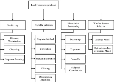
Load forecasting can be conducted by various methodologies. The selection of a forecasting method depends on so many factors including the relevance and availability of the historical data, the forecast horizon, the level of the accuracy for the weather data, the desired prediction accuracy and so forth. In general, the selected method and technique should make the best use of available data. Some of the most applicable methods for load forecasting in the literature can be categorized into the similar day method, variable selection method, hierarchical forecasting and weather station selection according to the Hong and Fan’s survey [2], whereas each approach looks at the forecasting problem uniquely.

Figure 1 shows the tree diagram of these four forecasting methods. As can be seen, each method can be carried out via multiple strategies. For example, there are various approaches to predict a hierarchical structure, i.e., bottom up, top down, ensemble and weighted combination. A full description of these four recognized categories of LF methodologies is represented in the following subsections with examples of several case studies.

Load Forecasting methods

Variable Selection Hierarchical Forecasting

Weather Station Selection

Bottom-up

Weighted Combination

Ensemble Top-down Similar day

Stepwise Method

Filtering Mutual Information

Correlation

Optimization Algorithm Distance

Minimization

Sequence Learning Clustering

Average Model

Optimal-number-of-stations Model

Figure 1. Tree Diagram of the Forecasting Methods

2.1. The Similar Pattern Method

Nearest Search Space

1 year ago

2 years ago now

Figure 2. limitation of search space for the similar days

Figure 3 illustrates the methodology applied by Dudek et al. [18] appropriately. In the first step, the similar days with the similar weekday index and day-of-the-year index as the forecast day extracted from the load time series (first series), as well as a sequence of the days following these similar days (second series). In the second step, the days with the similar patterns within the first series (similar-day series) were chosen by a selection strategy, and those followed by these newly selected days within the second series (sequence series). The outcome of the third step is a regression model of the load data extracted from the sequence series, and eventually, the next day in the original time series is forecasted by decoding the final model.

Besides the calendar index as the similarity indicator, other characteristics such as weather similarities can also be considered. For instance, Ying Chen et al. [19] proposed a similar-day selection method based on the weather similarity of the forecast day. In their proposed method which was designed to forecast the load in a short-term period (two working days excluding the weekend) by hourly resolution, the search for the similar days was limited to the days with the same weekday index and weather index to the forecast day. The days with similar weather condition were selected based on a minimization process, while the meteorological condition was defined by wind-chill, temperature, humidity, wind speed, and cloud cover variables. Also, the same index was assigned for some of the weekdays with similar load pattern. It also has been shown that relying only on the similar day’s data without establishing the initial status of tomorrow’s load leads to an inaccurate forecast result. Thus the 24-hour today’s load has been fed as an input to the forecast engine. Figure 4 illustrates the schematic diagram of the similar pattern method developed in [19].

Original load series

Extracted Similar days

Extracted sequences of similar days

Similar pattern selection

Decoding 1

1

2

3

4

Original Load Series

Weather Data Similar Pattern Loads

1

2 3

ANN

Today’s Load

Figure 4. Schematic Diagram of the similar pattern method developed by Chen et al. [19]

As already mentioned, the selection of the similar patterns between the days with similar indexes (weekday, the day of the year and weather indexes) can be made by a distance minimization technique. Some works in the literature applied Euclidean norm to measure the match level between the similar days [20] [12] [19]. As listed in table 1, Chen et al. [19] used the Euclidean norm to evaluate the weather similarity between the forecast day and previous days. Senjyu et al. [20] also applied a weighted Euclidian to investigate the similarity of load patterns using the load deviations between forecast day and historical days, weather deviation and the slope of load deviations. the assigned weights (w) in the formulae (2) is determined based on a regression model using the trend of load and temperature.

Dynamic Time Warping (DTW) is also another method to measure the similarity, for those time series with similar values not exactly at the same time point. Using the DTW method might end up finding more similar patterns of load profiles within the dataset. Teeraratkul et al. [21] indicated that by using the DTW method, the number of groups for similar profiles reduced by 50%.

Table 1. Distance minimization method for similarity measurement

Paper Method Formulae Parameters

[19]

Euclidean Distance minimizatio n

𝐦𝐢𝐧

𝒊 ∑ 𝒘(𝒕)

𝒇_{− 𝒘(𝒕)}𝒊 _, 𝟐𝟒

𝒕 𝟏 𝒊

(1)

: historical days f: forecast day i: historical day in 

𝒘: weather factor under consideration

[12] [20]

Weighted Euclidean Distance minimization

𝐦𝐢𝐧

𝒕 𝒘𝟏(△ 𝑳𝒕) 𝟐_{+ 𝒘}

𝟐(△ 𝑳𝒔)𝟐+ 𝒘𝟑(△ 𝑻𝒕)𝟐

(2)

△ 𝑳_𝒕: deviation of load of forecast day and historical day △ 𝑳_𝒔: deviation of slope between load on forecast day and load of historical day △ 𝑻𝒕: deviation of

More Recently, clustering algorithms are used to find similar load patterns within the dataset [22, 23]. These clustering techniques are used to group the data into a specific number of categories of the daily load patterns, naming the pattern-sequence based LF method. In this way, a label indexes the load for each day in the dataset. Consequently, a sequence of labels is created in the dataset. Alvarez et al. [24] applied K-means clustering technique to create clusters of different load patterns and extracted a sequence of labels from the dataset as a pattern to search within the dataset to predict the next day’s load. a schematic of pattern-sequence based forecasting method is depicted in figure 5. According to figure 5, all the weekdays in a dataset are labeled using a clustering method. To predict the next day’s load, a window of a sequence of labels before the forecast day is selected, then the same sequence of labels is searched within the dataset. By averaging the load of the next days, the load of the forecast day is achieved.

The prevalence of the smart meters in the smart grid facilitated the market planners with the fine-grained data with hourly and sub-hourly resolution. The load profiles at the customer-ends provide more sophisticated information about the type of customers and their consumption behaviors. Quilumba et al. [25] used a clustering technique to group the smart meter customers according to their similar energy pattern consumption. The temperature information was interpolated between the neighbor values to become as granular as the smart data.

2

3 2 3 1 42 32 2 3 1 4

1 ._. 2 1 ._. 2322 3 1 4X

5000 5500 6000 6500 7000 7500 8000 8500 12 :3 0: 00 01 :3 0: 00 02 :3 0: 00 03 :3 0: 00 04 :3 0: 00 05 :3 0: 00 06 :3 0: 00 07 :3 0: 00 08 :3 0: 00 09 :3 0: 00 10 :3 0: 00 11 :3 0: 00 12 :3 0: 00 01 :3 0: 00 02 :3 0: 00 03 :3 0: 00 04 :3 0: 00 05 :3 0: 00 06 :3 0: 00 07 :3 0: 00 08 :3 0: 00 09 :3 0: 00 10 :3 0: 00 11 :3 0: 00 5000 5500 6000 6500 7000 7500 12: 00 :0 0 01: 00 :0 0 02: 00 :0 0 03: 00 :0 0 04: 00 :0 0 05: 00 :0 0 06: 00 :0 0 07: 00 :0 0 08: 00 :0 0 09: 00 :0 0 10: 00 :0 0 11: 00 :0 0 12: 00 :0 0 01: 00 :0 0 02: 00 :0 0 03: 00 :0 0 04: 00 :0 0 05: 00 :0 0 06: 00 :0 0 07: 00 :0 0 08: 00 :0 0 09: 00 :0 0 10: 00 :0 0 11: 00 :0 0 5000 5500 6000 6500 7000 7500 8000 8500 Average Forecast day Window=4 4500 5000 5500 6000 6500 7000 7500 12 :00 :00 01 :30 :00 03 :00 :00 04 :30 :00 06 :00 :00 07 :30 :00 09 :00 :00 10 :30 :00 12 :00 :00 01 :30 :00 03 :00 :00 04 :30 :00 06 :00 :00 07 :30 :00 09 :00 :00 10 :30 :00 4500 5000 5500 6000 6500 7000 12 :00 :00 01 :30 :00 03 :00 :00 04 :30 :00 06 :00 :00 07 :30 :00 09 :00 :00 10 :30 :00 12 :00 :00 01 :30 :00 03 :00 :00 04 :30 :00 06 :00 :00 07 :30 :00 09 :00 :00 10 :30 :00 17 4500 5000 5500 6000 6500 7000 7500 12:00

:0001:30:0002:30:0004:30:0007:00:0006:30:0009:00:0012:00:00:0011:3001:30:0002:30:0004:30:00:0006:0007:30:0009:00:0010:30:0011:30:00 4/5 5000 5500 6000 6500 7000 7500 8000 8500 12:30:

0002:00:0003:30:0005:00:0006:30:0008:00:0009:30:0011:00:0012:30:0002:00:0003:30:0005:00:0006:30:0008:00:0009:30:0011:00:00

4500 5500 6500 7500 8500 9500 10500

1 72 143 214 285 356 427 498 569 640 711 782 853 924 995 1066 1137 1208 1279 1350 1421

Clustering

1 2 3 4

Figure 5. schematic of the pattern sequence-based forecasting method [24]

Clustering methods can distinguish the similar sequences within a dataset as discussed earlier; however, they cannot differentiate the main features of these patterns. More recently, adding memory to the structure of learning engines such as recurrent neural network and deep learning outweigh this drawback.

memory structure to adjust the length of the input and output sequences. A sequence to sequence structure is primarily designed to map sequences with different length [30] [31]. Marino et al. [31] discussed that the main advantage of the sequence to sequence structure is the ability of the approach to predict an arbitrary number of future time steps having an arbitrary length of an input sequence. Satish et al. [32] investigated the optimum learning sequence for the training stage. The results indicated that the number of patterns in a sequence impacts the accuracy of the model.

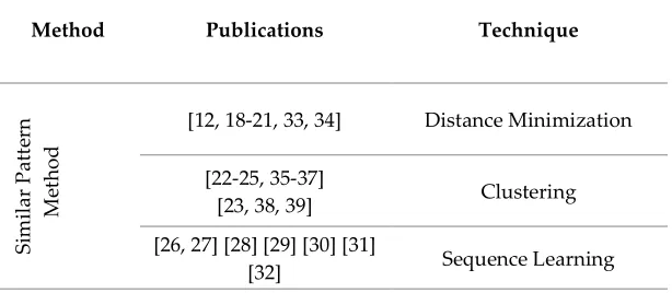
Table 2 lists the highly cited publications in which similar-pattern method was applied for load prediction. These publications are categorized based on the three common techniques of “distance minimization”, “clustering” and “sequence learning”.

Table 2. Published articles using the similar-pattern method

Method Publications Technique

Si

m

ila

r P

at

te

rn

M

et

ho

d

[12, 18-21, 33, 34] Distance Minimization

[22-25, 35-37]

[23, 38, 39] Clustering

[26, 27] [28] [29] [30] [31]

[32] Sequence Learning

On the whole, the pattern similarity method is a suitable method to capture the repeated patterns of the load series in a short-term. The overall pattern of a system is rarely changing in the short term; while in longer periods, some significant deviations might lessen the similarity of the future load to the past load.

2.2. The Variable Selection Method

Variable selection is the process of selecting the most influential variables or features (predictor variables) within the dataset that can adequately capture the relationship between the available data and the output model. Despite time series forecasting which only relies on the past data, the variable selection method determines the external variables besides the historical load to embed into the model [40].

Some of these variables- that are so-called explanatory variables due to explaining the reason of load fluctuations- are calendar variables (time of the day, day of the week, month of the year and day of the year etc.), meteorological variables (temperature, humidity, cloud cover, wind chill, solar radiation etc.), the historical load and so forth [41].

Several studies also considered the lagged load data into their model[42, 43]. The lagged variables determine the effect of recency by incorporating the alteration of demand level throughout the load time series into the model. For example, Ceperic et al. [42] proposed a feature selection algorithm to select the optimum number of the lagged loads in order to embed the sequential correlation of the load variables within the dataset into the model. Another example is the work of Fan and Hyndman [11] that considered the lagged load demand for each of the preceding 12 hours, and the lagged values for the same hours of the two previous days, as well as the maximum and minimum load values in the past 24 hours and average load in the previous week; Although, a selecting algorithm has chosen some of these candidate variables.

level of validation that partly depends on the weather station section which will be discussed more in the related section.

By nominating multiple input variables, considering the huge number of the available data for every variable, the predictor engine might not be able to converge to an accurate predictive model. Therefore, an effective subset of the data with the optimal number of predictor variables will help the forecast accuracy[44]. An effective predictor variable is highly explanatory and independent of other variables. The aim is to select the optimal subset of the predictor variables with fewer numbers that suitably describes the characteristics of the output variable. The optimal input subset favors the model accuracy, as well as the cost efficiency and model interpretability [45]. In the literature, researchers employed different methods and techniques to select explanatory variables optimally.

One of the methods used for variable selection is the stepwise refinement which is a step by step approach for selecting the inputs. In this method, the primary model is a full model consists of all the measured variables. Hence, based on the predictive capability of the individual variables, the redundant terms from the model will be omitted. The retained variables consequently lead to the best model. One example is the work of Fan and Hyndman [11] who carried out a step by step variable selection method to extract the best-suited model. The nominated inputs were the calendar variables, actual demand and lagged demand (from the National Electricity Market of Australia-NEM) and forecasted temperature data from more than one sites in the target area. For example, in the first stage, the temperature differentials form the same period of the last six days were dropped one at a time, and the one which led to the lowest error was selected. Consequently, in the next stage, the temperature variable has been frozen to only the selected day from the last stage, and the temperatures of the last six hours were considered for the trail. This procedure has been continued until the final group of variables was selected.

Nedellec et al. [46] followed the same strategy of stepwise refinement for variable selection as well, but in a three-step procedure while the variables in each stage were selected based on the scale of the forecast. In the long-term module, monthly load and temperature time series for every region and weather station were selected, to extract the long-term trend and low-frequency effects. The residual of the first stage with no seasonality and weather effects were considered for a medium-term estimate. Variables such as a type of the day, type of the year, de-trended electrical load, real temperature, and lagged temperature were the predictor variables in the medium-term model. In short-term stage, more localized factors that were remained were captured by selecting variables such as year, month, day, hour, time of the year and day type, as well as real and smoothed weather variables. This stepwise algorithm is illustrated in figure 6 for a better understanding. As can be seen, the final forecasted load is an additive model of the three components.

Model on Monthly Data (extract the trend)

Fit a Middle Term Model on Detrended Data

Fit a Short Term Correction Model on

Residuals

ZMt

ZLt ZSt

Trends Economical Factor Slow Changes in Electricity Usage

Meteorological Effects Calendar Effects Daily to weekly

Effects

Extreme Weather Network Reconfiguration

Holidays

Local Effects Monthy Effects

Zt

Figure 6. Step wise Algorithm for Load Forecasting [46]

There are also other approaches to identify the maximum relevance between different variables. Correlation-based methods use a heuristic algorithm to find the subset of variables that are highly correlated with the output but are not correlated with each other [48]. Chen et al. [9] used the correlation method to measure the dependency of the peak demand to the temperature. Kouhi et al. [49] developed a correlation-based feature selection method to reduce the chaotic structure of a load time series and selected the highly relevant variables within this reconstructed space. Amjady et al. [3] also used a correlation approach to create a subseries of the load data to develop a hybrid forecast model.

Mutual Information (MI) is an information theoretic-based approach to measure the interdependency between variables. Wang et al. [50] used the MI method to obtain the initial weights of the developed ANN based load forecast model. Elattar et al. [51] reconstructed a load time series by embedding the dimension and time delay computed by the mutual information approach. Young-Min Wi et al. [52] adopted the MI method to evaluate the mutual information between the dominant weather features and loads of the different seasons.

Moreover, Reis et al. [53] applied wavelet filter to reconstruct a subseries of data after selecting the input variables using autocorrelation function. Amjady et al. [54] also proposed a hybrid load prediction algorithm in which a filter-based technique selected a minimum subset of inputs. Zhongyi Hu et al. [55] proposed a hybrid filter method for the feature selection procedure.

More recently, developing the bio-inspired optimization tools as well as the evolutionary optimization algorithms leaded to improving the CI-based feature selection techniques for load forecasting. Some examples of the developed optimization algorithms for feature selection in the literature include Ant Colony [56], Particle Swarm [57, 58], Differential Evolution [59], hybrid Genetic and Ant Colony [60] and so forth.

Table 3. List of the publications using different feature selection techniques

Publication Technique

[11, 46][47] Stepwise

[53, 54] Filter

[3, 9, 45, 49, 61, 62] Correlation

[45, 50-52, 63] Mutual Information

[56] [57, 58] [59] [60, 64] Optimization Algorithms

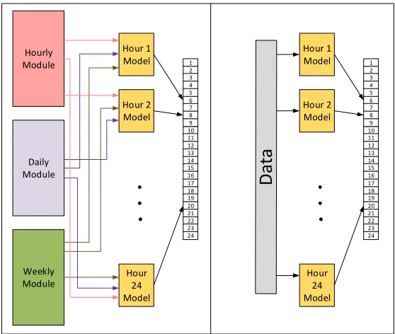
Generally, there are two main parts in forecasting a system. The first one is selecting the appropriate group of inputs; the other is to find a suitable architecture for the forecasting engine [65]. For example, Khotanzad et al.[66] proposed a three-module structure to model the hourly, daily and weekly trend by one of each. In their developed architecture for prediction of the hourly load of the next day, the decomposed result of each of the three modules would be trained by 24 ANN engines for each hour of the day.

Some other papers in the literature also applied the so-called parallel architecture for 24-hour ahead load forecasting [42, 67]. The reasons for utilizing this design are the smaller number of the training data for each module, the omitted parameters for the hour of the day, the simpler model for each hour of the day comparing to one general model for all 24 hours and so forth. Figure 7 shows an overview of the parallel design for 24-hour ahead load forecasting. The left side picture is a schematic of the architecture proposed by Khotanzad et al.[66].

Hourly Module

Daily Module

Weekly Module

Hour 1 Model

Hour 2 Model

Hour 24 Model

1 2 3 4 5 6 7 8 9 10 11 12 13 14 15 16 17 18 19 20 21 22 23 24

Hour 1 Model

Hour 2 Model

Hour 24 Model

1 2 3 4 5 6 7 8 9 10 11 12 13 14 15 16 17 18 19 20 21 22 23 24

Figure 7. Parallel Architecture for 24-hour ahead forecasting

the selection of the input variables. The forecaster’s experiences in analyzing the type of the data from a specific market, as well as the preliminary testing might help to select the proper group of variables. Thus, the professional judgment is undoubtedly part of the process.

2.3. Hierarchical Forecasting

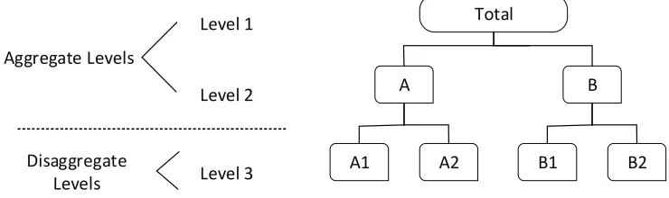
The previous methods presumed the load data as single time-series, while these time series can be inherently disaggregated by different attributes of interest [40]. Load time-series naturally are organized based on different hierarchies such as geographic, temporal, circuit connection and revenue. Figure 8 depicts a typical hierarchical structure of a time-series divided into aggregate and disaggregate levels.

One example of a hierarchical load structure can be found in a study conducted by Zhang et al. [68]. The load data was the recorded consumption of 300 smart meter customers of a subsection in Australian utility within 3 years. The 300 customers were clustered into 30 nodes with their postcodes. These 30 nodes again grouped into 3 nodes. Also, these three nodes summed up at final level to one aggregated time series. In the distribution level; however, the hierarchical levels are specified as the load of substations, feeders, transformers and, customers [69].

Total

A B

A1 A2 B1 B2

Aggregate Levels

Disaggregate Levels

Level 1

Level 2

Level 3

Figure 8. Schematic Diagram of the Hierarchical Structure of a load time series

Recently, there has been a prevailing attention to the hierarchical load model due to the market considerations for decision making in different levels of the power system including independent system operator, distribution operator, and the customer-ends. Utilities need the forecast at low voltage levels in order to perform effectively the operation at the distribution level such as circuit switching and load control. The accurate forecasting model at low level could even increase the prediction accuracy at independent system operator level [70]. In fact, the independent system operator in the upper level in a power system covers a large geographical area, with extensive load diversities throughout the area. Hence, a single model is not able to guarantee the prediction accuracy.

The state-of-the-art load forecasting methods to deal with hierarchical load structure are sub-grouped into bottom-up and top-down approaches [25, 71]. The bottom-up approach aggregates the forecasts form low level to the aggregated level, while the top-down method aggregates the historical load prior to the forecasting. The former approach doesn’t miss out any information due to the aggregation; although, high volatility of bottom level is challenging to be predicted [72]. The top-down method, on the other hand, is simpler for less noisiness due to the aggregation; although, some features for the individual series will be lost [40]. For instance, Quilumba et al. [25] used the bottom-up approach for forecasting the load of the customers disaggregated by the similar consumption patterns.

Hierarchical Load Forecasting can also be conducted at all levels of the hierarchies individually, that is so called as “base forecast”; however, here the challenge is that the prediction at aggregated level might not be consistent with the added up base forecast [74].

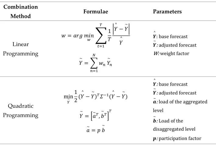
Zhang et al. [68] proposed a solution to optimally adjust the base forecasts at each node to be consistent across the aggregation structure. This goal has been accomplished by minimizing the redundancy between the forecast at the aggregated level and the sum of the base forecasts, using quadratic programming in a post-processing scheme. The method was tested on two electricity networks, one bulk system of a large area with several dispatch zones at the bottom level, the latter is a distribution network covering a small area with hundreds of individual customers at a low level. The result shows that for more than 85% of the nodes in bulk network, the proposed method was more accurate. For distribution network with more volatile load, the improvement is more obvious especially at the upper aggregated level the error is significantly decreased. Nose-Filho et al. [75] developed a load model for a sub-distribution system in New Zealand as well by finding participation factors between the local forecasts and the global forecast.

Another example is the study by Fan et al. [76] who proposed a strategy to forecast the load of the sub-regions within a large geographical area independently by finding the optimal region partition in the combination procedure. It has been argued in [76] that the weather condition is a dominant factor on load variations; therefore, the extreme variation in weather condition throughout the area can be interpreted as high load diversity with the large region. The other factor that makes the regional load profiles to be vastly different has been identified to be the noncoincident load peaks.

Sun et al. [69] proposed a strategy to predict loads of different nodes in a distribution power system, by a top-down approach. First, loads of parent nodes are forecasted, then by finding the similarity between the parent node (aggregated level) and its child nodes (correspondent disaggregated levels), two classes of regular and irregular nodes are identified. Thus, for the regular nodes, the load is a fraction of the origin load, calculated by a distribution factor. For those irregular loads which do not follow the leading characteristics of the parent node, individual models are forecasted. The similarity between nodes was identified by using the distance minimization method, for both the weather parameter and the historical load.

More recently, with the dominance of smart meters, fine-grained data at sub-levels reveal more information at the aggregated level. Wang et al. [77] used the granular smart meter data to construct a forecast model at an aggregated level. In their proposed model, the data is clustered into different groups of loads with similar patterns, and the aggregated forecast is obtained by adding up the forecast of the individual clusters; however, instead of the bottom-up strategy, a weight is assigned to each model while varying the number of clusters. The final forecast is an optimally weighted combination of these individual forecasts. Their proposed method was implemented on a data set consists of 5237 residential consumers’ data with half hourly resolution for 75-week duration. It has been shown that the result of the direct aggregated load is more accurate than the clustering strategy; while, their proposed method outweighs both other methods. Besides this data set, the method was also tested on 155 substations load data for the 103-week duration. In contrast to the first data set, the outcomes indicate that the bottom-up model is more accurate than other individual clustering models. It has been concluded that the reason for this contrast is due to regularity in substation load in comparison to residential load profiles.

Table 4. Combination Methods for base forecasts Combination

Method Formulae Parameters

Linear Programming

𝑤 = 𝑎𝑟𝑔 𝑚𝑖𝑛 1

𝑇 𝑌^− 𝑌~

𝑌^

𝑌~= 𝑤 𝑌~

𝒀^: base forecast 𝒀~: adjusted forecast

W: weight factor

Quadratic Programming

min_~ 1 2(𝑌

^

− 𝑌~) 𝛴 (𝑌^− 𝑌~)

𝑌~= 𝑎~ , 𝑏~

𝑎~= 𝑝 𝑏~

𝒀^: base forecast 𝒀~: adjusted forecast

𝒂~: load of the aggregated

level

𝒃~: Load of the disaggregated level

𝒑: participation factor

Different levels of a hierarchical structure interact with each other in a complicated fashion, whereas a change in one series at one level, can change the series at the same level as well as other levels of a hierarchy sequentially. Sun et al.[69] considered the change that switching operation might cause on the load trend, by adjusting the forecast as the switching is detected. The abnormal changes in the demand were identified by measuring the mean and standard deviation of the load using statistical process control, and then the load participation factor is calculated based on the new data. Comparably, deviations in the meteorological conditions in a large geographical area cause the base forecasts to vary, leading to the changes in the aggregated load accordingly. However, the meteorological information might not be available at every sub-level. there are a number of meteorological services available at a geographical area, providing the weather forecast information. Hong et al. [79] argued that in a hierarchical structure with various nodes to be forecasted, the best-related weather information could not be selected manually for each node. The method of weather station selection was one of the main objectives in the Global Energy Forecasting Competition 2012 (GEFC) [80]. More about this is discussed in the next section.

2.4. Weather Station Selection

In a large electricity market covering an expanded area, a single forecasting model cannot capture the load pattern. The hierarchical structure that was discussed in the previous section ensure a more satisfactory forecast across different levels of hierarchy. However, in a hierarchical structure that disaggregates the load based on geographical divisions or zonal hierarchies, the meteorological hierarchies that are for sure a dominant factor in load diversity cannot easily be captured. The challenge is to assign the most related weather station information to each zone or area in the hierarchy.

Fan et al. [76] proposed a combination method to select the best adapted individual weather forecast between multiple forecasts provided by different meteorological services. several papers in the literature [81, 82] used the average data from multiple services for its simple and effective result comparing to other weighted averaging methods.

Between the winning teams, Charlton et al. [83] built 11 energy model for each zone based on the weather data of 11 weather station provided in the competition. The best-fitted weather station for each zone is not a single station. Instead, it is a linear combination of up to 5 best-fitting weather stations for each group. Lloyd [84] also developed a forecast model based on all the weather stations’ data and used a Bayesian model averaging to integrate these models into one final average model. Moreover, In the proposed model by Nedellec et al. [46], one station was selected for each zone, considering that other combination strategies led to unsatisfactory outcomes. Taieb et al. [85] selected the best-fitted station for each zone by testing the last week temperature data for each zone. The demand modeled using the average temperature data of best three weather sites.

Hong et al.[79], on the other hand, proposed a method for weather station selection, that instead of assigning the same number of weather station to all nodes at the same level of hierarchy (as it was the common strategy in the GEFC competition), different numbers of weather stations are selected for individual load zones; Although, the result was not always superior to other alternatives.

3. Method Evaluation and Future Work

A comprehensive explanation of the LF methodologies provided in the last sections. Generally, the logic behind every specific method helps the forecaster to choose the best-fitted method based on their application. For example, the similar pattern method mainly relies on the historical values, in spite of the variable selection method which incorporates the information about explanatory variables. Therefore, the forecaster might consider the similar pattern method where the system might not be comprehensive enough, or if it is explanatory, it is extremely difficult to extract the main features that govern the demand behavior. In this situation, there are always some variations in the load that cannot be captured by explanatory variables. In similar pattern strategy, on the other hand, the focus is on what is going to happen rather than why it happens. still, when there is a correlation between exogenous variables and load data, explanatory model i.e. variable selection method is a suitable approach.

Some of the main advantages and disadvantages of these four methods are listed in Table 5. For example, in the variable selection method, as one drawback, it is assumed that all the input variables are independent of each other; although, in reality, they are partly correlated. To some extent, inserting some lag information as input data partly captures the high correlations between variables. Similar pattern method, on the other hand, presumes that the past values of a variable are important in predicting the future; although, the algorithms can only look back for a few steps for a limited sequence of data.

Table 5. Advantages and disadvantages of the load forecasting methodologies

Method Advantage Disadvantage

Similar Pattern Method

 Adapt to exceptionalcircumstances and random events

 No previous knowledge about the system is needed

 The horizon of forecast is immitted up to a couple of days

ahead

 Limited search space  Not explanatory

Variable Selection Method

 Embedding exterior variables into the model

 Increase prediction accuracy by reducing overfitting and addressing the

curse of dimensionality

 No comprehensive correlation between variables

 Simpler prediction (smaller number of predictors or smaller size of input

space)

 Improves the understanding of the prediction model

 Redundancy

 Non-independent input variables

Hierarchical Method

 help the power system operators to perform the load control and circuit

switching at different levels of the

hierarchies.

 Enhancing the model accuracy by using the information at the lower levels

 Lack of coherency across the aggregated structure.  Loss of information due to

aggregation in the top levels  The high irregular data at the

bottom levels of the hierarchies

Weather Station Selection

 Find the best fitted weather data for each level of the hierarchy

 Uncertainty about Optimal number of stations for each

hierarchy

Hyndman et al.[73] discussed that taking advantage of the prominent features of different methods and combine them in a hybrid scheme is what we need to do now. Some examples of this combination are available in the literature.

For example, Quilumba et al. [25] applied the similar pattern method in one step to group the smart meter load profiles into an optimal number of groups and the feature selection method in the next step to forecast the aggregated load at each group of data.

In the proposed load model by Wang et al. [77] a three-stage combined model has been applied. The hierarchical structure of the load series extracted by applying the hierarchical clustering technique based on the similar consumption behavior of the customers. Different load models developed at each subgroup of the data using variable selection method, and eventually the final model revealed by adding a weight factor to the individual models in order to be coherent across the aggregate level.

Another example of the hybrid methodology can be found in the work of Zheng et al. [29], in which the feature selection method is used to help to find the similar days’ clusters. Each cluster is shaped based on the feature values of the data, whereas a weighted parameter is assigned to each feature.

distance again at the aggregate level. Further assessment is required as a future work to evaluate the feasibility of this method on actual load data.

Aggregate Level

Disaggregate Level

1

1

3 The Similar Pattern Days _{The Similar Pattern Days}

Create Different Combination Of The Similar Pattern Days 2

2

4 Find The Combined Patterns With The Minimum Distance 5

6 Forecast The

Next Day’s Load 7

Figure 9. Schematic diagram of the proposed hybrid method

4. Conclusions

In this paper, the state-of-the-art methodologies for load forecasting divided into four main categories are discussed. Each of these methods proposes a specific solution for LF. Similar pattern method that is rooted form the minimum distance method, presumes that the load trend is unlikely to vary during a short period; Hence, by searching within the close vicinity of today’s load, some similar patterns can be distinguished. In fact, forecasting the future load is based on the subsequent behavior of the discovered similar patterns in the load series.

Variable selection method, on the other hand, tries to find the prominent, independent features in a dataset with the lowest correlation with each other and high correlation with the output. Constructing a subseries of these features help to improve the forecast accuracy.

Other methods, on the other hand, deal with the aggregate loads in different levels of the hierarchical structure. Predicting the load in various zonal level help the power system operators to effectively perform the switching operation and load control. In addition, improving the forecast at sub levels enhances the prediction accuracy at upper levels.

Besides the geographical and zonal hierarchies, the weather hierarchy is another vital factor in load forecasting that cannot be captured easily for each geographical zone. various weather services in a large geographical area provide different weather forecast information. Selecting the best-suited weather information is substantially important for load forecasting considering the influence of weather variables on the load trend.

Eventually, by highlighting the main advantages and disadvantages of each method, it has been concluded that combining the single methods in the hybrid scheme can benefit from the robustness of the single techniques. In the end, the simple outline of a hybrid strategy is proposed for future evaluation.

Author Contributions: Seyedeh Narjes Fallah came up with the primary idea. The initial idea further developed with the collaboration of Mehdi Ganjkhani and Shahaboddin Shamshirband. The contribution is as following: methodology, S.N. Fallah; investigation, S.N. Fallah, M. Ganjkhani, S. Shamshirband; supervision, S. Shamshirband; original draft preparation: S.N. Fallah; writing and editing: S.N. Fallah, M. Ganjkhani, S. Shamshirband; and and Kwok-wing Chau visualization: M. Ganjkhani, S. Shamshirband;

Nomenclature

ANN Artificial Neural Network

ARIMA Auto-Regressive Integrated Moving Average ARMA Auto-Regressive Moving Average

CI Computational Intelligence DTW Dynamic Time Warping

GEFC Global Energy Forecasting Competition LF Load Forecasting

MI Mutual Information RNN Recurrent Neural Network

SARIMA Seasonal Auto-Regressive Integrated Moving Average SVM Support Vector Machine

References

1. Shahidehpour, M., H. Yamin, and Z. Li, Market operations in electric power systems: forecasting, scheduling, and risk management. 2003: John Wiley & Sons.

2. Hong, T. and S. Fan, Probabilistic electric load forecasting: A tutorial review. International Journal of Forecasting, 2016. 32(3): p. 914-938.

3. Amjady, N., Short-term hourly load forecasting using time-series modeling with peak load estimation capability. IEEE Transactions on Power Systems, 2001. 16(3): p. 498-505.

4. Khotanzad, A., et al., ANNSTLF-a neural-network-based electric load forecasting system. IEEE Transactions on Neural networks, 1997. 8(4): p. 835-846.

5. Huang, S.-J. and K.-R. Shih, Short-term load forecasting via ARMA model identification including non-Gaussian process considerations. IEEE Transactions on power systems, 2003. 18(2): p. 673-679.

6. Pappas, S.S., et al., Electricity demand loads modeling using AutoRegressive Moving Average (ARMA) models. Energy, 2008. 33(9): p. 1353-1360.

7. Lee, Y.-S. and L.-I. Tong, Forecasting time series using a methodology based on autoregressive integrated moving average and genetic programming. Knowledge-Based Systems, 2011. 24(1): p. 66-72.

8. Chakhchoukh, Y., P. Panciatici, and L. Mili, Electric load forecasting based on statistical robust methods. IEEE Transactions on Power Systems, 2011. 26(3): p. 982-991.

9. Chen, B.-J. and M.-W. Chang, Load forecasting using support vector machines: A study on EUNITE competition 2001. IEEE transactions on power systems, 2004. 19(4): p. 1821-1830.

10. Khosravi, A., et al., Interval type-2 fuzzy logic systems for load forecasting: A comparative study. IEEE Transactions on Power Systems, 2012. 27(3): p. 1274-1282.

11. Fan, S. and R.J. Hyndman, Short-term load forecasting based on a semi-parametric additive model. IEEE Transactions on Power Systems, 2012. 27(1): p. 134-141.

12. Mandal, P., et al., A neural network based several-hour-ahead electric load forecasting using similar days approach. International Journal of Electrical Power & Energy Systems, 2006. 28(6): p. 367-373.

14. Moghram, I. and S. Rahman, Analysis and evaluation of five short-term load forecasting techniques. IEEE Transactions on power systems, 1989. 4(4): p. 1484-1491.

15. Raza, M.Q. and A. Khosravi, A review on artificial intelligence based load demand forecasting techniques for smart grid and buildings. Renewable and Sustainable Energy Reviews, 2015. 50: p. 1352-1372.

16. Fallah, S., et al., Computational intelligence approaches for energy load forecasting in smart energy management grids: state of the art, future challenges, and research directions. Energies, 2018. 11(3): p. 596.

17. Mu, Q., et al. Short-term load forecasting using improved similar days method. in Power and Energy Engineering Conference (APPEEC), 2010 Asia-Pacific. 2010. IEEE.

18. Dudek, G., Pattern similarity-based methods for short-term load forecasting–Part 1: Principles. Applied Soft Computing, 2015. 37: p. 277-287.

19. Chen, Y., et al., Short-term load forecasting: similar day-based wavelet neural networks. IEEE Transactions on Power Systems, 2010. 25(1): p. 322-330.

20. Senjyu, T., et al., One-hour-ahead load forecasting using neural network. IEEE Transactions on power systems, 2002. 17(1): p. 113-118.

21. Teeraratkul, T., D. O’Neill, and S. Lall, Shape-based approach to household electric load curve clustering and prediction. IEEE Transactions on Smart Grid, 2018. 9(5): p. 5196-5206.

22. Iglesias, F. and W. Kastner, Analysis of similarity measures in times series clustering for the discovery of building energy patterns. Energies, 2013. 6(2): p. 579-597.

23. Seem, J.E., Pattern recognition algorithm for determining days of the week with similar energy consumption profiles. Energy and Buildings, 2005. 37(2): p. 127-139.

24. Alvarez, F.M., et al., Energy time series forecasting based on pattern sequence similarity. IEEE Transactions on Knowledge and Data Engineering, 2011. 23(8): p. 1230-1243.

25. Quilumba, F.L., et al., Using Smart Meter Data to Improve the Accuracy of Intraday Load Forecasting Considering Customer Behavior Similarities. IEEE Trans. Smart Grid, 2015. 6(2): p. 911-918.

26. Liu, C., et al. Short-term load forecasting using a long short-term memory network. in Innovative Smart Grid Technologies Conference Europe (ISGT-Europe), 2017 IEEE PES. 2017. IEEE.

27. Kong, W., et al., Short-term residential load forecasting based on resident behaviour learning. IEEE Transactions on Power Systems, 2018. 33(1): p. 1087-1088.

28. Shi, H., M. Xu, and R. Li, Deep learning for household load forecasting–a novel pooling deep RNN. IEEE Transactions on Smart Grid, 2017.

29. Zheng, H., J. Yuan, and L. Chen, Short-term load forecasting using EMD-LSTM neural networks with a Xgboost algorithm for feature importance evaluation. Energies, 2017. 10(8): p. 1168.

30. Sutskever, I., O. Vinyals, and Q.V. Le. Sequence to sequence learning with neural networks. in Advances in neural information processing systems. 2014.

31. Marino, D.L., K. Amarasinghe, and M. Manic. Building energy load forecasting using deep neural networks. in Industrial Electronics Society, IECON 2016-42nd Annual Conference of the IEEE. 2016. IEEE.

32. Satish, B., et al., Effect of temperature on short term load forecasting using an integrated ANN. Electric Power Systems Research, 2004. 72(1): p. 95-101.

33. Barman, M., N.D. Choudhury, and S. Sutradhar, A regional hybrid GOA-SVM model based on similar day approach for short-term load forecasting in Assam, India. Energy, 2018. 145: p. 710-720.

35. Jin, C.H., et al., A SOM clustering pattern sequence-based next symbol prediction method for day-ahead direct electricity load and price forecasting. Energy Conversion and Management, 2015. 90: p. 84-92.

36. Panapakidis, I.P., Clustering based day-ahead and hour-ahead bus load forecasting models. International Journal of Electrical Power & Energy Systems, 2016. 80: p. 171-178.

37. Goia, A., C. May, and G. Fusai, Functional clustering and linear regression for peak load forecasting. International Journal of Forecasting, 2010. 26(4): p. 700-711.

38. Mori, H. and T. Itagaki. A precondition technique with reconstruction of data similarity based classification for short-term load forecasting. in Power Engineering Society General Meeting, 2004. IEEE. 2004. IEEE.

39. Verdú, S.V., et al., Classification, filtering, and identification of electrical customer load patterns through the use of self-organizing maps. IEEE Transactions on Power Systems, 2006. 21(4): p. 1672-1682.

40. Hyndman, R.J. and G. Athanasopoulos, Forecasting: principles and practice. 2018: OTexts.

41. Lusis, P., et al., Short-term residential load forecasting: Impact of calendar effects and forecast granularity. Applied Energy, 2017. 205: p. 654-669.

42. Ceperic, E., V. Ceperic, and A. Baric, A strategy for short-term load forecasting by support vector regression machines. IEEE Transactions on Power Systems, 2013. 28(4): p. 4356-4364.

43. Espinoza, M., et al., Short-term load forecasting, profile identification, and customer segmentation: a methodology based on periodic time series. IEEE Transactions on Power Systems, 2005. 20(3): p. 1622-1630. 44. May, R., G. Dandy, and H. Maier, Review of input variable selection methods for artificial neural networks, in

Artificial neural networks-methodological advances and biomedical applications. 2011, InTech.

45. Koprinska, I., M. Rana, and V.G. Agelidis, Correlation and instance based feature selection for electricity load forecasting. Knowledge-Based Systems, 2015. 82: p. 29-40.

46. Nedellec, R., J. Cugliari, and Y. Goude, GEFCom2012: Electric load forecasting and backcasting with semi-parametric models. International Journal of forecasting, 2014. 30(2): p. 375-381.

47. Xiao, J., et al., A hybrid model based on selective ensemble for energy consumption forecasting in China. Energy, 2018. 159: p. 534-546.

48. Hall, M.A., Correlation-based feature selection of discrete and numeric class machine learning. 2000.

49. Kouhi, S., F. Keynia, and S.N. Ravadanegh, A new short-term load forecast method based on neuro-evolutionary algorithm and chaotic feature selection. International Journal of Electrical Power & Energy Systems, 2014. 62: p. 862-867.

50. Wang, Z. and Y. Cao. Mutual information and non-fixed ANNs for daily peak load forecasting. in Power Systems Conference and Exposition, 2006. PSCE'06. 2006 IEEE PES. 2006. IEEE.

51. Elattar, E.E., J. Goulermas, and Q.H. Wu, Electric load forecasting based on locally weighted support vector regression. IEEE Transactions on Systems, Man, and Cybernetics, Part C (Applications and Reviews), 2010. 40(4): p. 438-447.

52. Wi, Y.-M., S.-K. Joo, and K.-B. Song, Holiday load forecasting using fuzzy polynomial regression with weather feature selection and adjustment. IEEE Transactions on Power Systems, 2012. 27(2): p. 596.

53. Reis, A.R. and A.A. Da Silva, Feature extraction via multiresolution analysis for short-term load forecasting. IEEE Transactions on Power Systems, 2005. 20(1): p. 189-198.

54. Amjady, N. and F. Keynia, Short-term load forecasting of power systems by combination of wavelet transform and neuro-evolutionary algorithm. Energy, 2009. 34(1): p. 46-57.

56. Niu, D., Y. Wang, and D.D. Wu, Power load forecasting using support vector machine and ant colony optimization. Expert Systems with Applications, 2010. 37(3): p. 2531-2539.

57. Lin, S.-W., et al., Particle swarm optimization for parameter determination and feature selection of support vector machines. Expert systems with applications, 2008. 35(4): p. 1817-1824.

58. Hu, Z., Y. Bao, and T. Xiong, Comprehensive learning particle swarm optimization based memetic algorithm for model selection in short-term load forecasting using support vector regression. Applied Soft Computing, 2014. 25: p. 15-25.

59. Amjady, N., F. Keynia, and H. Zareipour, Short-term load forecast of microgrids by a new bilevel prediction strategy. IEEE Transactions on smart grid, 2010. 1(3): p. 286-294.

60. Sheikhan, M. and N. Mohammadi, Neural-based electricity load forecasting using hybrid of GA and ACO for feature selection. Neural Computing and Applications, 2012. 21(8): p. 1961-1970.

61. Liang, Y., D. Niu, and W.-C. Hong, Short term load forecasting based on feature extraction and improved general regression neural network model. Energy, 2019. 166: p. 653-663.

62. Santos, P., A. Martins, and A. Pires, Designing the input vector to ANN-based models for short-term load forecast in electricity distribution systems. International Journal of Electrical Power & Energy Systems, 2007. 29(4): p. 338-347.

63. Ghadimi, N., et al., Two stage forecast engine with feature selection technique and improved meta-heuristic algorithm for electricity load forecasting. Energy, 2018. 161: p. 130-142.

64. Hong, W.-C., et al., SVR with hybrid chaotic immune algorithm for seasonal load demand forecasting. Energies, 2011. 4(6): p. 960-977.

65. Swarup, K.S. and B. Satish, Integrated ANN approach to forecast load. IEEE Computer Applications in Power, 2002. 15(2): p. 46-51.

66. Khotanzad, A., R. Afkhami-Rohani, and D. Maratukulam, ANNSTLF-artificial neural network short-term load forecaster-generation three. IEEE Transactions on Power Systems, 1998. 13(4): p. 1413-1422.

67. Kalaitzakis, K., G. Stavrakakis, and E. Anagnostakis, Short-term load forecasting based on artificial neural networks parallel implementation. Electric Power Systems Research, 2002. 63(3): p. 185-196.

68. Zhang, Y., J. Wang, and T. Zhao, Using Quadratic Programming to Optimally Adjust Hierarchical Load Forecasting. IEEE Transactions on Power Systems, 2018.

69. Sun, X., et al., An efficient approach to short-term load forecasting at the distribution level. IEEE Transactions on Power Systems, 2016. 31(4): p. 2526-2537.

70. Hong, T. and M. Shahidehpour, Load forecasting case study. EISPC, US Department of Energy, 2015. 71. Capasso, A., et al., A bottom-up approach to residential load modeling. IEEE Transactions on Power Systems,

1994. 9(2): p. 957-964.

72. Stephen, B., et al., Incorporating practice theory in sub-profile models for short term aggregated residential load forecasting. IEEE Transactions on Smart Grid, 2017. 8(4): p. 1591-1598.

73. Hyndman, R.J., et al., Optimal combination forecasts for hierarchical time series. Computational Statistics & Data Analysis, 2011. 55(9): p. 2579-2589.

74. Gamakumara, P., et al., Probabilistic Forecasts in Hierarchical Time Series. 2018, Monash University, Department of Econometrics and Business Statistics.

75. Nose-Filho, K., A.D.P. Lotufo, and C.R. Minussi, Short-term multinodal load forecasting using a modified general regression neural network. IEEE Transactions on Power Delivery, 2011. 26(4): p. 2862-2869. 76. Fan, S., K. Methaprayoon, and W.-J. Lee, Multiregion load forecasting for system with large geographical area.

77. Wang, Y., et al., An ensemble forecasting method for the aggregated load with sub profiles. IEEE Transactions on Smart Grid, 2018.

78. Yang, Y., Combining forecasting procedures: some theoretical results. Econometric Theory, 2004. 20(1): p. 176-222.

79. Hong, T., P. Wang, and L. White, Weather station selection for electric load forecasting. International Journal of Forecasting, 2015. 31(2): p. 286-295.

80. Hong, T., P. Pinson, and S. Fan, Global energy forecasting competition 2012. 2014, Elsevier.

81. Xie, J., et al., Relative humidity for load forecasting models. IEEE Transactions on Smart Grid, 2018. 9(1): p. 191-198.

82. Liu, B., et al., Probabilistic load forecasting via quantile regression averaging on sister forecasts. IEEE Transactions on Smart Grid, 2017. 8(2): p. 730-737.

83. Charlton, N. and C. Singleton, A refined parametric model for short term load forecasting. International Journal of Forecasting, 2014. 30(2): p. 364-368.

84. Lloyd, J.R., GEFCom2012 hierarchical load forecasting: Gradient boosting machines and Gaussian processes. International Journal of Forecasting, 2014. 30(2): p. 369-374.