Binomial type sums

VICTORIA ~

UNIVERSITY

•

' z ~

z 0 ~ 0 0 ~

DEPARTMENT OF COMPUTER AND

MATHEMATICAL SCIENCES

Binomial Type Sums

P. Cerone and A. Sofo

(58MATH10)

June, 1995

(AMS: 05A10, 40C99)

TECHNICAL REPORT

VICTORIA UNIVERSITY OF TECHNOLOGY

(P 0

BOX 14428) MELBOURNE MAIL CENTRE

MELBOURNE, VICTORIA, 3000

AUSTRALIA

TELEPHONE (03) 9688 4249

I

4492

FACSIMILE (03)

9688 4050

BINOMIAL.SUM

BINOlVIIAL TYPE SUMS

P. CERONE AND A. SOFO

VICTORIA UNIVERSITY OF TECHNOLOGY

P. 0. BOX 14428, MELBOURNE MAIL CENTRE,

MELBOURNE, AUSTRALIA, 3000

BINOMIAL TYPE SUMS

Abstract

Using ideas from residue theory, a method is developed which in turn allows a specific finite

Binomial type sum to be expressed in closed form. The binomial type sum has applications in

the areas of network reliability and discrete distributions.

AMS: 05A10, 40C99

Introduction

Some ideas of residue theory are used in expressing a finite sum in closed polynomial form.

The sum to be considered is

(-lt+m

~)-lY(n)rn+m

(n+m)!

r=O

r

and it arises in the study of differential-difference equations in the work of Sofo and Cerone

(to appear).

Binomial sums have been considered by Gould (1994) and the sum of the powers of natural

numbers has been considered by de Bruyn (1995). Binomial type sums considered in this

paper are related to Stirling numbers of the second kind, which in tum are related to Bernoulli,

second order Eulerian and Bell numbers. However, the readers need not be acquainted with

any of these special numbers

as

the authors develop a recurrence relation to determine the finite sum. The binomial type sum considered here has applications in the areas of network

reliability, see for example the work of Prekopa et al. (1991) and in the representation of a

discrete distribution, see the work of Brandt et al. (1990).

Firstly, in this paper, an infinite double sum is obtained from which a recurrence relation is

developed. Then it is shown that the double sum may be expanded in a Maclaurin series.

Secondly it is proved that the finite sum above can be written as a polynomial inn of degree

·Background and problem statement

Volterra integral equations of the form

'V(t)

=

F(t)

+

J;'V(t-x)<j>(x)dx

(1)

occur in a wide area of applications, (e.g. Tijms (1986)), as do differential-difference equations

of the first order with a shift parameter, (e.g. Bellman and Cooke, (1963)).

Taking the Laplace transform of (1) and putting

F(t)

= 8(t), the Dirac delta impulse function,

will produce an expression of the form

'I'( ) -

1

p -1-<l>(p) (2)

Taking the Laplace transform of a differential-difference equation of the first order will

produce a result like (2).

Now consider the rectangular wave

<j>(x)

= H(a-x) = l-H(x-a), where H(x) is the

Heaviside function. The Laplace transform of

<j>( x)

is:

1 -ap

i.

{<j>(x)}

=

<l>(p)

=

-e

p

and the

n

-th moment of

<j>( x)

is given by

Substituting (3) into (2) results in

'I'( ) -

p

p - 1 -ap

p- +e

An expansion of (5) gives

(3)

(4)

(5)

00

It may be noticed that

'l'(p)

can be written in the form

'l'(p)

=

LJ3m(a)pm

m=O where

In this paper the finite sum over

r

in equation (7) will be investigated.

A Recurrence Relation for

J3m (a)

J3m (a)

may be given alternatively, from (5), as

J3m(a)

=

lim[-

1

~{

\ )}] ;

m

= 1,2,3 ... .

p~O

m

!

dpm

1- <I>

p

and in particular

J3

0

(a)

=

1

( )

= -

1

-;a

*

1.

1-<I> 0

1-a

Furthermore, using the ideas developed by Cerone (1994),

I - .

dm [

<l>(p) ] .

-

.

m.J3m(a)-lim-

l+ ( ) , m-1,2,3 ... .

p~O

dpm

1-<I>

p

r

dm [

<l>(p) ]

=

/!]

dpm

1-<l>(p)

Hence, using (4) and (8) then, (9) may be written as

that is, the

J3m (a)

are given by the recurrence relation

(7)

(8)

(9)

(10)

m-1 m-(k-1)

(1-a)J3m(a)=

I/-lt-k (

~(

_ ))

1

.J3k(a);

m=l,2,3....

(11)

k=O m

k

1 .

1

From (7),

oo n+m

~m(a)=

I/-lf+m

(a

)

1

.

s(m,n)

n=O

n+m .

where

s(m,n)=

l(-1r(;)r"+m.

r=O

00 j

Puttingj

=

n+ m

gives

~m(a)

=

I/-l)i

~s(m,j-m)

j=m J.

m oo j

=(-It~s(m,O)+

L

(-l)i

~s(m,j-m).

m. j=m+l J.

Since,

s(m,O)=

t,<-1r(~}

0

-

=

0,

m

;0 0, then

00 j

~ ·a

~m(a)= ~(-1)1-.

1

s(m

,

j-m)

j=m+l J ·

and so the problem lends itself in trying to express ~m

(a)

as a Maclaurin series.

From (7) and (12),

Pm

(a)

may be expanded in a Maclaurin series

(12)

(13)

and the coefficients ~m

(q)(O)

can be calculated from the recurrence relation in (11), as follows.

From the left hand side of (11)

-{(1-a)Pm(a)}-

dq _ ~ -(1-a).~m q

(q)

dq-r (r)

(a),q-0,1,2, ...

. _

daq

£:t

r daq-r .

and this term is zero only for

r

=

q and

r

=

q -1, so that

(14)

-5-The last expression can be written as the sum of two terms corresponding to the a0 _{term for}

r

=

q - m

+

k - 1 and to the ai , j ?:. 1, term for r > ( q - m

+

k - 1). .,,

Hence,

!!!__[Ic-1r-k

am-k+l

Pk(a)]= lC-1r-k(

q

)P~q-m+k-l)(a)

daq k=o

(m-k+l)!

k=o

q-m+k-l

+

I:c-1r-ki(q)

am-k+l-(q-r)

.pr)(a).

k=O

r=o r (m-k+l-(q-r))!

(15)

Now, setting a=

0

in

(14)

and

(15)

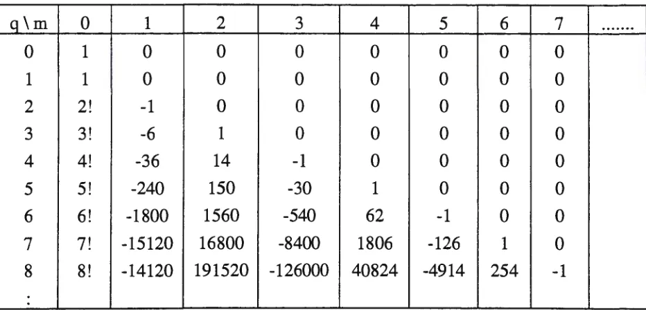
gives, after equating the right hand sides, the following

recurrence relation for the coefficients of the Maclaurin series

(13),

p(q)(o)-qp(q-l)(o) =

~c-1r-k(

q k

1

).p~q-m+k-l)(o),

q=0,1,2,

....

(16)

m m £..i

qm+

-k=O

These coefficients are demonstrated in Table 1.

q\m

0

1

2

3

4

5

6

7

'

0

1

0

0

0

0

0

0

0

1

1

0

0

0

0

0

0

0

2

2!

-1

0

0

0

0

0

0

3

3!

-6

1

0

0

0

0

0

4

4!

-36

14

-1

0

0

0

0

5

5!

-240

150

-30

1

0

0

0

6

6!

-1800

1560

-540

62

-1

0

0

7

7!

-15120

16800

-8400

1806

-126

1

0

8

8!

-14120 191520 -126000

40824

-4914

254

-1

.

Table 1 : Coefficients of p~l

(

0)

Some observations that may be made from

(16)

and table 1 are as follows:

The Polynomial

It will now be shown that the coefficients of the power series for ~m

(a)

have the following property.

Theorem:

_{The fimte sum} . _{Pm ( n) = (} (-l)"+m )

2,. (

n

-1)'

( n rn+m is a polynomial in n of ) n+m

!

r=o r

degree

m.

Proof:

From (7),

~m(a)

=

i~~+nl(O)

am+n

+

i(-l)"+m an+m t(-1Y(n)rn+m. (17)

n=l (m+n)! n=m+l (n+m)! r=O r

From (11),

m = 1,2,3, ....

(-Itam+I [

1

(m+l)a

2 (m+l)ma3(a+2) (m+l)m(m-l)a4(l+2a)

=

- +

2

+

2 3

+

3 4

(m+l)!(l-a)

l-a 2a(l-a) l2a

(l-a)

24a

(l-a)

(m+l)m(m-l)(m-2)a5(6+32a+8a2-a3) (m+l)!am ( )]

+

4(

s

+ ... +

1(

)mXa

3 ! 5 ! a l - a) 2am- 1- a

where the function

X(a)

is a polynomial in

a,

to be detennined from the particular ~m-l

(a).

That is,

( ) (-ltam+I

[c

)m-1

(m+l)a(l-at-2

(m+l)ma(a+2)(l-at-3

~ a = l-a

+

+

+

m (

m

+

1)

!(

1-

a

r+l

2 12

(m+ I)m(m-I)a(l +2a)(l-at-4 (m+ l)m(m-I)(m-2)a(

6+32a+8a

2 -a3)(I-at-s

_:.___;__.: __ _;___;,_ _________

+---~

24

3!5!

(m+l)!a

]

+ ... +

-7-+(m+1)m(m-1)(m-2)~(-l)k(m-5)[

₆

_{k+r 32 k+}2

8 k+3 _ k+4 ] (m+l)!aX(a)}

3

_{· ·}

151 .£..i

_k=O

k a + a + a a + ... . ₂

- (-1)

2m

~(n+m)

n+m+l{ m-1[ 1 m+l (m+l)m (m+l)m(m-l)(m-2) ]

-

""-'

a

a

-

+ - - - + +

(m+l)!n=O n 2 12 3!5! ....

+am-2[(m-l)- (m+ l)(m-2) + (m+ l)m(m-1) + ... ]

2

12

+ ...

.

...

ao[ ... ]}.

Thus, ~m (a) may be expressed in the form

13.

(a)=~(

n: m ){ a••2• F;(m) + a••2m-t F,(m)+ ... +a••m+t

F.

(m)}

where the ~(m),j = 1,2, .... ,m, are functions dependent on the fixed parameter m only.

The summation indices are now adjusted to obtain coefficients of common powers of a in the

following manner.

A

(a)

=

~

(n

+

1

)an+m+l

R (

m)

+

~

(n

+

2

)an+m+l

E (

m)

Pm £..i n - m

+

1 1 £..i n - m

+

2 . 2

n=m-1

n=m-2

L

oo

(n

+

m

-

l}n+m+IF ( )

Loo

(n

+

m}n+m+l F ( )

+ ...

+

1 m-1 m

+

m m '

n-

n

and SO,

+ ...

.

. .

Grouping of terms gives

A ( )

~

n+m+t[(n+l ) ( ) (n+2 ) ( (n+m-1) (n+m)

J

!-',.,. a

=

f:;,a n-m+l

F;.

m + n-m+2 Fi m)+ ... + n-1 F,,,_,(m)+ n F,.,.(m)

and SO,

~

n+m [ (

n )

(n

+

1 )

(n

+

m

-

2)

(n

+

m

-1)

.

J

~,,.(a)= nf:+~ n-m F;_(m)+ n-m+l Fi(m)+ .... + n-2 Fm_,(m)+ n-1 F,.,.(m)

m

+

_Lan+mGm+l-n(m)

(19)

n=l

where the functions

Gj(m),

like

Fj(m),

are dependent only on the fixed parameter

m.

From the right hand side of (17) and (19) it may be seen that,

m m~ m

~

A(m+n)(O)

a

-

~

m+kG

(m)

~1-'m (

)!

~a

m+I-k

n=I m+n · k=l

(20)

and equating the powers of

am+

j , where j

=

m

+

1, m

+

2, ...

(-l)"+m

~(-lY(n)r"+m

=

~(n+k

)F.

(m)

.

( +

n m .

)

,~ r=o r ~ k=O n-m+k

k+I

-9-Now since,

., (n+k n-m+k

)=

(n+k)(n+k-1) ... (n+k-m+l). _

_m.

₁

,k-0,l,2

,

... ,(m-l)

is a polynomial in n of degree m and the ~+i ( m) functions depend on the fixed parameter m,

then the right hand side of (21) is a polynomial inn of degree

m.

Hence,

Pm(n)

=

(-1r+m

f,(-1y(n)r"+m

(n+m)! r=o r

(22)

is a polynomial in n of degree m, and the theorem is proved.

Finite differences may be used to determine a specific polynomial, however the following procedure establishes a recurrence relation to determine the values of ~+i

(m)

in (21).

Relations between ~~)(O),Gk(m) and ~+

1

(m)

From (18) and (19) it can be seen that, on equating coefficients of

am+j

,j = 1,2, ... ,m gives,

and therefore

m-k(m+

jy,

Gk(m)

=

L .

j+k(m),

k

=

1,2,3, ... m.

The functions

F;(m)

;

j

=

1,2, ... :m, in (21) can now be recursively obtained from

MF=G ₍₂₃₎

where

M

is an ( m x

m)

upper triangular matrix,

F and G

are ( m x

1)

column vectors.

Similarly, from (20)

~<m+k)(O)

Gm-k+

1

(m)

=

(~+k)!

; k=l,2,3, ...

m.

Now, putting q

=

m

+

k

~(q)(O)

Gzm-q+I

(m)

=

m

'

q. q = m+I,m+2, ... 2m,

and for the counter j = 2m - q

+

1

~~m+I-j)(O)

Gj

(m)

;

j = m,m-1,m-2, ... ,3,2,I,

(2m+l-j)!

where the ~~)(O) values can be obtained from (16).

Therefore (23) may be written as

MF= ~~m+I-k)(O) I (2m+ 1-k) ! ; k

=

1,2,3, ... m, or

(~)

(m~l)

(m;z)

...

(z:=D

]\(m)

~~m)(O) I (2m) ! ~~m+l)(O) /(2m+ 1)!

(~)

( m

~

1) ...

.(2:=;)

Fz(m)

= (24)

(~)

(m~l)(m~2)

_{Fm_z(m)}

_{' ~:+}3_l(O)/(m+3)!

(~)

(m;l)

_{Fm_}

This matrix setup therefore allows a recursive evaluation of the functions

~(m);

j =

1,2,3, .... m, in terms of the coefficients ~~)(O) in the Maclaurin series (13).

From the work of the previous section

F; (m)

takes the form

(m+l)!F;(m) =-l+ m+l

(m+l)m

+O+

(m+l)m(m-l)(m-2)

_{+ ... (25)}

2

12

6!

and for a particular value of

m,

that same number of terms are used on the right hand side of (25).

1

1

1

Therefore

F; (

1) = - - ,

F; (

2) = -

,

F; (

3) = 0,

F; (

4) = - - ,

Fi (

5) = 0, ....

and because of the

2

12

6!

f01m of the polynomial in table 2, for every m;;?:: 3 and odd only, it is conjectured that

.F;(m)

= 0. Of course all

F;(m)

values can be evaluated from (24).

Examples

(A) Let m = 3 and from (21) and (22)

R()

(-lf+

3

~(-l)r(n)rn+3=~(n+k

)F. (

3)

3 n (

_{n+ .}

3) 1 "'-' r "'-' n - 3

+

k k+l

r=O k=O

From (24) and table 1,

(

3)

0

r17 3

(3) =

~~4)(0)

4!

= _

_!_.

4!' 0

(3)R (3)+

2

(4)R

1

3

(3) =

~;s)(O)

5!

-

30 .

5! '

R

2

(3) =- 10

5!

and hence

( n )

(n+l)( 10) (n+2)( 1)

n

2

(n+l)

~(n)

=

n-3

(O)+

n-2

-5!

+ n-1 -

4!

=-

2.4!

and

(-1r

:tc-1r(n)rn+3 = n

2

(B) The following example uses the idea of a multi.nominal distribution.

Consider

n

different coloured marbles in each of

(n

+

3)

bags. In how many ways can one draw a marble from each bag such that all coloured marbles are represented in the 'hand' of

(n

+

3)

marbles?

From the multinominal distribution, the total number of ways this can be done is:

= (n+

3) ![n2(n

+

1)]

2.4! (27)

From the inclusion - exclusion principle, the total number of ways can be written down as

However, from the work of the previous section

(-1)" ic-1r(n)r"+3

=~(n)=

n2(n+l)

(n+3)!

r=O r 2.4!

so that

which is equivalent to (27).

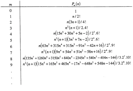
-13-Table 2, below lists the sum (22) in closed polynomial form for the values

of m = O,l,2,3,4,5,6, 7,8,9.

m

1

n/2!

n(3n+ 1)/ 4!

n2(n+l)/2.4!

n(15n3 +30n2 +5n-2)/23.6!

n2(n+1)(3n2 +7n-2)/24.6!

0 1 2 3 4 5 6 7 8 9

n( 63n5 +315n4 + 315n3 -9ln2 -42n+16) / 23• 9 !

n2

(n+1)(9n4 +54n3 +5ln2 -58n+16)/24.9!

n(135n1_+1260n6 _+3150n5 _+840n4

-2345n3 +540n2 -404n-144) /3.27 .10!

n2_(n+1)(15n6 _+165n5

+465n4-17n3 -648n2 +548n-144)/3.28.10!

Table 2 : Some examples of Pm

(n)

in closed form

These polynomials are related to the Stirling polynomials, see Graham et al. ((1989), by

n'

Pm(n) ( · ) S(n+m,n)

n+m !

where S(p, q) is the Stirling number of the second kind. From table 2, ~ ( 4)

=

513. Using

the table on page 835 of Abramowitz and Stegun (1965), S(7,4)=350 and hence

P(4)

=

4

!

.350=~.

3

7! 3

In the next section a generalization of (22) is given whereby noninteger values may be

summed.

A Generalization

Consider

Qm(n,x)

tl)'~

i<-1Y(n)(x+rt+m

n+m !r=o r

(28)

The following lemma is needed.

Lemma

R;(n)=

~(-I)'(~)e ={~-I}'n!

i=0,1

,

2

,

... ,(n-1)

(29)

z =n

Proof

From the expression

(1-y)"

=

~(~)<-1)'y',

differentiating i times gives

:ii

{(1-yf} = (-lYn(n-1) ..

.

... (n-i+l)(l-y)"..;

i

=

ic-1t(~)k

i

l-

i

;

for

i=0,1,2

,

..

..

(n-1)

,

y

k=O

and so putting y = 1, results in

Further for i

=

n ,

differentiating

n

times gives

(-l}'n!=

~(-!)'(~}·.

From (28)

Qo(n,x)

= (-l)" ic-1r(n)(x+r)"

=ii

(-lY+"

(n)(n)x"-krk

(30) n ! r=o r r=o k=O n ! r k

-Expanding and adding down columns results in

Qi(n

,

x)

=

x"

(-1)"

(n)i(-ll(n)ko

+

x"-1

(-l)"

(n)i(-l)k(n)k

1 +

x"-2

(-l)"

(n)t(-l)k(n)kz

n

! 0

k=o

k

n

! 1

k=o

k

n

! 2

k

=

o k

x

0

( -1 )"

(n) "

k

(n)

n

-15-Now, utilising the above lemma, from (29)

_xn(-IY(n)

x1

(-1Y(

n)

x

0

(-IY(n)

n

Q0

(n,x)-

₀

.O+ .

.

... +

1

.O+

.

(-1)

n!

n! n!

n-

n!

n

and hence, from (30)

Q

₀

(n,x)=

(-ir

i(-1y(n)(x+rY

=l.

n!

r=o

r

(31)

The result in (31) can be integrated m times with respect to x to produce the result

Qm(n,x)at

(28).

The closed form of (28) can now be obtained as follows, integrating (31) and using the initial

condition Q_{1 (}

n,

0)

=

Pi (

n)

=

!!:. ,

from table 2 for

m

= 1, results in

2

Q,

(n, x)

=

(-I)~

:±,

(-I)'(n)(x

+

r

y+i

=

.!.(n

+

2x)

(n+

1 !

r=o

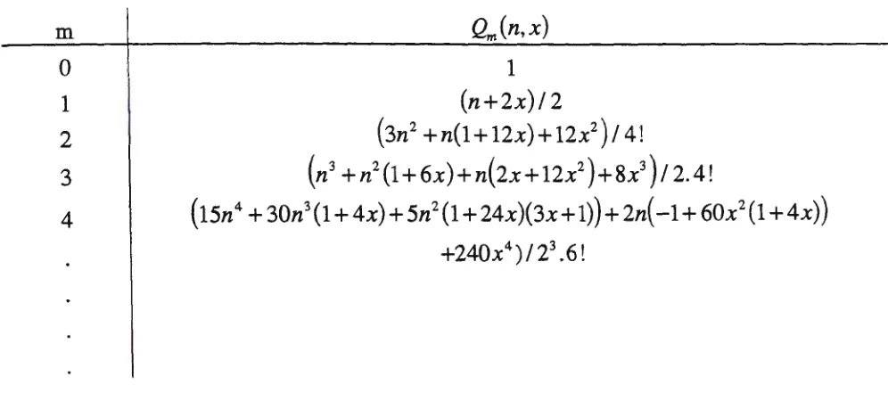
r

2

Using this procedure, table 3 below is given listing

Qm (

n, x)

which gives (28) in closed form.

From (28)

so that the coefficients of

xi

can be expressed as

a .=

(-1r+m

(n~m)i(-1Y(n)rn+m-i;0-5.j-5.(n+m),

1

_(n+m)!

₁

_r=o

_r

(32)

-16-However, from (32), a i

=

0 for m

+

1

s; j s;

n

+

m using the lemma (29), and hence

(2m

(n, x) is

a polynomial in

x

of degree

m.

From the work of the previous section and above, Qm

(n,x)

is

a polynomial in n and x of degree m for both n and x.

m

0

1

2

3

4

1

(n+2x)/2

(3n

2

+n(1+12x)+12x

2) /

4I

(n

3

+n

2

(1+6x)+n(2x+12x

2

)+8x

3

)!

2.4!

(15n

4

+30n

3

(l +4x)+5n

2

(1 +24x)(3x+ l))+ 2n(-1+60x

2

(1 +4x))

+240x

4)/23

.6!

-Conclusion

A technique has been developed whereby Binomial type sums of powers can be expressed in

closed form. An application to the multinominal distribution has been given.

Acknowledgments

The authors are indebted to Dr. D. Watson for pointing out the application of the Binomial

type series to the multinominal distribution as in example (B), and to A. Glasson for helpful discussion.

References

Abramowitz M. and Stegun I.A. (1965). Handbook of Mathematical Functions,

New York, Dover.

Bellman

R.

and Cooke

K.L.

(1963). Differential-Difference Equations, New York,

Academic Press.

Brandt A, Brandt M, and Sulanke H. (1990). A representation of a Discrete Distribution by

its Binomial Moments, J. Appl. Prob. 27, 208.

Cerone P. (1994). On Series Involving zeros of Transcendental Functions Arising from

Volterra Integral Equations, V.U.T. Technical Report, 50 MATH 8.

l

_fi

2 2 p 3 3 p 11 p p·b .

De Bruyn G.F.C. (1995). Formu as or a+a +a + ... +an , 1 onacc1

Quarterly, 33 (2), 98.

Gould H. W. (1994). A Class of Binomial Sums and a Series Transform, Utilitas Math.

45, 71.

Graham R.

L.,

Knuth

D.E.,

and Patashnik

0. (1989).

Concrete Mathematics,

Addison-Wesley, Sydney.

Prekopa A., Boros

E.

and Lih

K.

W.

(1991).

The Use of Binomial Moments for Bounding

Network Reliability, Rutcor Research Report 6.

Sofo A., and Cerone P. (To Appear) Sums of Series using the Asymptotic behaviour.

Tijms H. C. (1986). Stochastic Modelling and Analyses: A Computational Approach,