Volume 32, Number 3 (May 1979)

JOURNAL OF

RANGE

MANAGEMENT

PublIshed bimonthly-January, March, May. July, September, November-by the

Society for Range Management 2760 West Fifth Avenue Denver, Colorado 80204 Copynght 1979 by the Society for Range Management

Managing Editor

LORENZ F. BREDEMEiER 2760 West Fifth Avenue Denver, Colo. 80204

Editor

REX D. PIEPER

Dep. Animal and Range Science New Mextco State Unlvensty Las Cruces, N Mex 88003

Book Review Editor

PAT 0. CURRIE

Science & Education Admin. Livestock and Range Research Station Route 1, Box 3

Miles City, Montana 59301

Copy Editor

PATRICIA G. SMITH 2760 West Fifth Avenue Denver, Colo. 80204

Editorial Board 1977-79

JAMES 0. KLEMMEDSON, Tucson, Ariz. GEORGE W. SCOTTER, Edmonton, Alta., Canada M.J. TRLICA, Fort Collins, CO

J. ROSS WIGHT, Sidney, MT 1978-80

DONALD A. KLEBENOW, Reno, NV JAMES T. NICHOLS, North Platte, NE MICHAEL D. PITT, Vancouver, B.C., Canada RONALD E. SOSEBEE, Lubbock, TX

1979-81

ROD BOVEY, College Station, TX NEIL FRISCHKNECHT, Provo, UT MARTIN VAVRA, Union, OR HAROLD GRELEN, Pineville, LA

INDIVIDUAL SUBSCRIPTION IS by membership In the Society for Range Management.

LIBRARY or other INSTITUTIONAL SUBSCRIPTIONS, on a calendar year basis, are $22.00 postpaid to all countries. Payment from outside the United States should be remitted In US dollars by tnternational money order or draft on a New York bank.

CHANGE OF ADDRESS notices should be sent to the Managing Editor, 2760 West Fifth Ave., Denver, CO 80204, no later than the first day of the month of issue. Copies lost due to a change of address cannot be replaced unless adequate notice IS given. To assure uninterrupted service, provide your local postmaster with a Change of Address Order (POD Form 3575), Indicating thereon to guarantee forwarding postage for second class mall POSTOFFICE: Please return entire journal with address change. BUSINESS CORRESPONDENCE, concerning subscnp- tons, advertising, reprints,, back Issues, and related mat- ters, should be addressed to the Managing Editor, 2760 West Fifth Ave., Denver, CO 80204.

EDITORIAL CORRESPONDENCE, concerning manu- scripts or other edltonal matters, should be addressed to the Editor, Dep. Animal and Range Sciences, New Mexico State Univ., Las Cruces 88003.

INSTRUCTIONS FOR AUTHORS appear each year In the March Issue, copies of these InstructIons are available from the editor.

SECOND CLASS POSTAGE paid at Denver, Colorado.

TABLE OF CONTENTS:

Vol. 32, No. 3, May 1979

ARTICLES 168

171

175

179

182

185 189

194

A96

201

209

21-l

116

‘21

116

130 ‘Z’ _c _

1.38

Growth Rates of a Cheatgrass Community and Some Associated Factors by D. W. Uresk, J.F. Cline, and W.H. Rickard

Utilization Practices and the Returns from Seeding an Area to Crested Wheatgrass by E. Bruce Godfrey

Seasonal Food Habits of White-tailed Deer in the South Texas Plains by Leroy A. Arnold, Jr. and D. Lynn Drawe

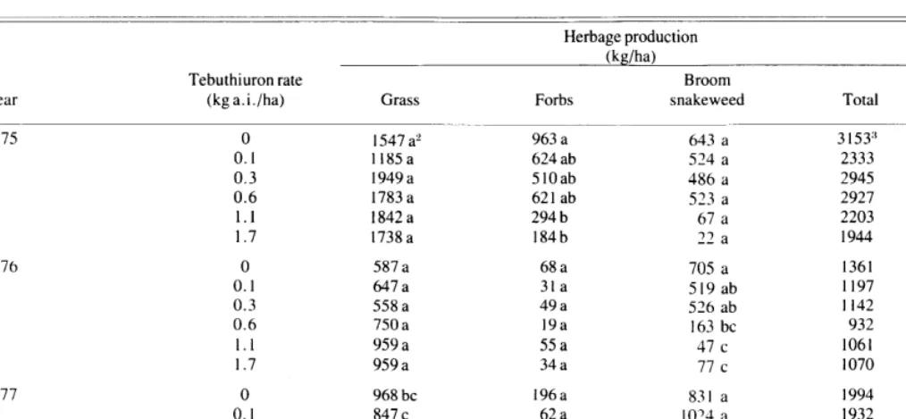
Broom Snakeweed Control with Tebuthiuron by Ronald E. Sosebee, W.E. Boyd, and C.S. Brumley

Productivity of Irrigated Tropical Grasses under Different Clipping Frequencies in the Semidesert Region of the Sudan by Ahmed E. Osman

Huisache Control by Power Grubbing O.E. Bontrager, C.J. Scifres, and D.L. Drawe Probable Impacts of Various Range Improvement Practices on Diffuse Salt Production by lradj K. Hessary and Gerald F. Gifford

Clipping of Water-stressed Blue Grama Affects Proline Accumulation and Pro- ductivity by karin Wisiol

Effects of Picloram and Tebuthiuron Pellets on Sand Shinnery Oak Communities by R.D. Pettit

An Explanation of the Bolivian Highlands Grazing * Erosion Syndrome by Allen LeBaron, Larry K. Bond, Percy Aitken S., and Leon Michaelsen

Seminal and Adventitious Root Growth of Blue Grama Seedlings on the Central Plains by A.M. Wilson and D.D. Briske

Winter Cold Damage to Bitterbrush Related to Spring Sheep Grazing by Charles H. Jensen and Philip J. Urness

Broom Snakeweed: Effect on Shortgrass Forage Production and Soil Water Depletion by Darrell N. Ueckert

Feeding Ecology of Feral Horses in Western Alberta by R. E. Salter and R. J. Hudson Forage Diversity and Dietary Selection by Wintering Mule Deer by L. H. Carpenter, O.C. Wallmo, and R.B. Gill

Assessing the Hazard of Picloram to Cutthroat Trout by D.F. Woodward Possible Impacts of the Expected Shift from Cow-Calf to Cow-Yearling Enter- prises by Suliman H. Abdalla and John P. Workman

Komondor Guard Dogs Reduce Sheep Losses to Coyotes: A Preliminary Evalu- ation by Samuel B. Linhart, Ray T. Sterner, Timothy C. Carrigan, and Donald R. Henne

TECHNICAL NOTES

111 The Literature of Range Science Based on Citations in the Journal of Range Management by John F. Vallentine

BOOK REVIEWS

Growth Rates of a Cheatgrass Community

and Some Associated Factors

D.W. URESK, J.F. CLINE, AND W.H. RICKARD

Abstract

Abiotic and biotic factors were found to be related to growth rates of a cheatgrass sward using stepwise regression analyses. Soil temperature and plant tissue nitrogen showed a strong relation with growth rates from initiation of growth to peak production. After peak production, soil temperature was related to declining growth rates. Water stored in the soil profile had a weak relationship with growth rates and plant growth was com- pleted before soil water became limiting. Equations were developed using soil temperature, nitrogen content of plant tissues, and live herbage production to estimate future production of cheatgrass.

Cheatgrass (Bromus tectorum) is common throughout the rangelands of southcentral Washington and utilized by cattle in late winter and early spring. However, production varies from year to year, depending upon weather conditions between October and June. The dynamics of cheatgrass growth as related to abiotic and biotic factors is an important aspect of short-term management of arid rangelands in the Pacific Northwest. The relationship between precipitation and peak standing crop of range forage plants has been investigated by Smoliak ( 1956), Sneva and Hyder (1962), Currie and Peterson (1966), Rauzi ( 1964), Albertson (1966), Hulett and Tomanek (1969), and S hiflet and Dietz ( 1974). Dahl ( 1963) related total yield of herbage with precipitation of the previous 2 years, evapotrans- piration, and predicted yields from soil moisture. Cable (1975) found that perennial grass production in Arizona was primarily dependent upon summer rainfall. Uresk, et al. ( 1975) related the amount of live herbage production, leaf moisture, and air temperatures to rates of growth rather than to peak standing crop for blue grama grass.

This paper examines soil water, soil temperature, and mineral content of tissues as factors showing a relationship or causative effect on the growth of cheatgrass in south-central Washington over a 5-year period, 197 1- 1975.

Study Area and Methods

The study area is an abandoned agricultural field located on the Arid Lands Ecology (ALE) Reserve on the Department of Energy’s Hanford Reservation (Cline and Rickard 1973; Rickard et al. 1976). The field supports a uniform sward of cheatgrass mixed with some minor species such as tansy mustard (Descuruiniapinnata) and tumble mustard (Sisymbrium altissimum). Prior to agricultural practices, the

Author\ are research biologist. U.S. Forest Service, Forestry Research Laboratory, South Dahota School ot Mines and Tech. Rapid City. South Dakota 57701; and senior rc\carch technologist and senior research scientist at Battelle. Pacific Northwest Labora- torlc\. RIchland. Washington 99.15’.

Thi\ worh was conducted by Battelle-Northwest Laboratories for the U.S. Department of Energy under contract E(45- I )- 1830. Thanks are extended to V. Charles, H. Sweeney, L. Kendall. M. Combs, and F. Nelson for their technical assistance.

Manuscript received April 17, 1978.

168

plant’ community was representative of the Artemisia tridentata/-

Agropyron spicutum association (Daubenmire 1970). The soi1 is

silt-loam with very few stones in the upper meter of its profile. The climate is semiarid, with an average annual precipitation of 17 cm from October to May. There has been little or no grazing by livestock since the field was abandoned in 1943.

Two sites, each 0.1 ha in size were established near the center of the field. Herbage was harvested by hand from ten randomly located 20 x 50 cm (0.1 m’) quadrats in each site. Sampling was conducted at 3-week intervals throughout the spring growing season and once during the fall. Live herbage was hand separated from the dead material by species. The herbage was oven dried for 48 hours at 6O”C, weighed, and analyzed for total nitrogen, phosphorus, and potassium (U.S. Testing Company).

Percentage soil water (dry basis) was determined gravimetrically in soil samples collected at I-dm increments to a depth of 8 dm using a barrel-type auger. Percent moisture was multiplied by bulk density to obtain soil water by volume. Soil temperature was measured by a recording thermograph with temperature sensing elements buried at 4 dm.

Statistical analyses for stepwise regression followed Draper and Smith ( 1968). Herbage data were combined over 3 years (197 1, 1972, and 1973) for these analyses, using site means by harvest dates. Regression equations related daily changes in amounts of herbage; factors were herbage weight (WT), plant nitrogen (N), phosphorus (P), potassium (K), soil temperature (T) at 4 dm depth, and soil water (W) at 1 -dm increments to 8 dm in depth. These data were separated into two periods of growth for analyses. First, regression equations were developed from the beginning of growth to peak biomass of cheatgrass and this interval is referred to as the accelerated growth period. Secondly, regression equations were determined from peak biomass to the end of growth, which is referred to as the senescent period.

The regression equations developed may be used to estimate future daily change in herbage weight of cheatgrass up to a maximum of three weeks. These equations were developed from the first three years of data and then tested on two independent years of data collected for 1974 and 1975. Only those independent variables that contributed significantly to the variation in the dependent variable (daily change in biomass) are presented in this study.

Results

The average maximum biomass production of cheatgrass during the 5 years (197 l-l 975) was 224 g/m’ (Table 1). The extreme low, 132 g/m’, occurred in 1972 while the peak high occurred in 1974 with 328 g/m”. The average rate of growth to peak biomass production was 2.9 g/m2/day for three years ( 197 1 - 1973). After peak production, the live tissues decreased at an average value of 3.8 g/m’/day. Precipitation during November to April was lowest for the 1973 season with 11 cm of water; highest November to April precipitation occurred during the 1974 growing season with 26 cm.

Table 1. Seasonal biomass values of cheat&v= @/m2h nitrogen content of tissues and soil temperature during the years 1971-1975.

Table 2. Regression equations showing the influence of biotic and abiotic factors on daily growth rates (P) of live cheatgrass from initiation of growth to peak herbage production (accelerated growth period) and

Year Herbage Nitrogen Soil temp (C”)

MO-Da XkSE’ % 4dm

post-peak herbage production (senescent period) to cessation.

Equation R2

1971

3-08 35.52 2.9 1.95 3.9

4-o 1 59.6+ 5.7 1.56 8.5

4-19 126.9+ 7.8 1.30 11.2

5-07 198.42 11.7 0.95 15.4

5-28 124.9kll.l 0.57 21.0

1 l-10’ 47.5+ 5.9 2.08 7.5

1972 3-14 4-03 4-13 4-25 5-15

56.3+ 4.1 2.31 9.8

76.42 2.6 1.48 10.3

131.7% 6.6 1.11 10.5

126.22 5.5 1.00 13.2

112.1+20.2 1.03 19.0

1973

3-06 32.02 3.2 2.25 7.8

3-26 36.42 2.3 2.10 9.5

4-06 70.42 5.2 2.14 12.8

4-23 115.1+11.3 1.83 15.5

5-07 165.8211.2 1.18 17.3

5-18 62.22 6.8 1.70 16.5

1974

3-13 78.0+ 4.7 2.04 7.0

4-l I 143.6+ 7.5 1.23 8.5

4-28 253.lkl4.1 0.64 13.0

5-22 328.0? 16.1 0.40 17.2

1975

3-20 60.02 6.8 2.60 4.8

4-28 193.02 7.6 1.13 10.0

5-13 294.5t18.6 0.54 14.1

6-06 221.4? 15.4 0.40 21.0

’ Mean c standard error. ’ Regrowth of cheatgrass.

Nitrogen content in live tissues ranged from 0.40% to a high of 2.60% (Table 1). Nitrogen content was highest early in the growing season with values exceeding 2%. Peak yield of plant nitrogen ranged from 1.5 to 2.2 g/m’ during the 5 years. Average peak yield of nitrogen in cheatgrass was 1.920.1 g/m* (+ SE). Soil temperatures at a 4-dm depth ranged from a low of 3.9” to 2 1 .O”C during the harvest periods from 197 1 to 1975 (Table I ).

In the cheatgrass community, 50% of the variation in changes during the spring period of accelerated growth was accounted for by the amount of live herbage present (WT) (Equation 1, Table 2), while the amount of live herbage accounted for48% of the variation during the senescent period (Equation 4). These equations may be used to estimate growth rates when soil temperatures or plant nitrogen are not available.

Soil temperature (T) accounted for 44% of the variation in daily growth (Equation 2, Table 2), and soil temperature and nitrogen (N) accounted for 77% of the variation (Equation 3). During the late fall of each year after soil water is replenished, soil temperature appears to influence or show a relationship with plant growth. Soil temperature may be the most reliable single factor to estimate growth rate until 11°C is reached. At temperatures above 1 l”C, nitrogen begins to influence or show a relationship with plant growth. Then Equation 3 is best used to estimate growth rates until a temperature of 15°C is obtained or approximately 0.5% nitrogen is present in the

Accelerated Growth Period

9 = 0.224 + 0.038 (0.0096)’ WT’ 0.50** 9 = -0.971 + 0.393 (0.114)T 0.44** f = 5.61 + 0.345 (0.077)

T - 3.211 (0.726)N 0.77** Senescent Period

9 = 6.68 - 0.06 (0.028) WT 0.48* ? = 13.86- 1.209(0.3887)T 0.66**

’ ( ) Standard error

’ WT = The amount of live herbage at a given time; T = Soil temperature at 4 dm;

N = Nitrogen content. * Significant at (~50. IO “* Significant at a50.01.

cheatgrass tissues. The decrease in live herbage was a function of soil temperature (Equation 5), which accounted for 66% of the variability. Soil temperature was the most highly correlated independent variable of all parameters associated with growth rates of cheatgrass during the senescent period. Soil water in the upper meter of soil profile did not contribute significantly to daily growth rates of cheatgrass biomass during both growth periods in the stepwise regression analyses.

Soil water as related to daily growth rates of cheatgrass showed differences by depth when comparing the accelerated growth and senescent periods (Table 3). Soil water showed a significant relationship with growth rates during the accelerated growth period to a depth of 9 dm. However, during the senescent period, late in the growing season, growth rates were significantly related with soil water only to a depth of 4 dm. Higher correlation coefficients (r) are shown for the senescent period; however the lower soil depths are not significant which may be due to a smaller sample size. Cline et al. (1977) showed that, in years where adequate soil moisture is available, soil water is not fully exploited by cheatgrass at the lower depths below 4 dm. During 197 I- 1973, the growth of cheatgrass had terminated before deeply stored soil water was used. However, during the drier years when soil water did not penetrate below the 5 dm soil profile, growth was limited primarily by soil water, rather than temperature and plant nitrogen.

The estimated values of biomass for the growing seasons of 1974 and 1975 were obtained from Equations 2,3, and 5, which

Table 3. Correlation coefficients (r) of soil water with growth rates of cheatgrass during the accelerated growth and senescent periods of her- bage production at I-dm increments to a depth of 10 dm.

Soil depth (dm)

Accelerated

growth period Senescent period

O-l -0.60* 0.86*

l-2 -0.59* 0.85*

3-3 -0.60* 0.77*

3-4 -0.59* 0.75*

4-5 -0.58* 0.73

5-6 -0.57* 0.72

6-7 -0.56* 0.74

7-8 -0.55* 0.73

8-9 -0.50* 0.72

9-10 -0.48 0.66

330

30

330

270

90

30

NOV DEC JAN FEB MAR APR MAY JUN JUL

Fig. 1. Abiotic and bioticfactors which were most influential in estimating the growth of cheatgrass are presented and a comparison of estimated versus actual biomass values during the 1974 and 1975 growing seasons.

were developed for years 197 1- 1973 (Table 2). Changes in herbage growth rates were predicted at future weekly intervals and these values were summed for each week to obtain total biomass. Reasonable agreement was shown between estimated and actual biomass values throughout the growing season for both years (Fig. 1).

Discussion

Temperature affects the qualitative and quantitative develop- ment of plants. The structural development and physiological processes of a plant may vary greatly with the temperature of the environment, depending on species. The annual growth of cheatgrass falls into three seasonal phases as related to soil temperatures-limited, relatively unaffected, and inhibited. The limited phase is defined as that period when temperature is not sufficient to allow optimum development of the plant. The relatively unaffected phase is that period where temperatures are favorable for optimum plant growth, while the inhibited phase is defined as that period when excessive temperatures retard or inhibit plant growth (Jarvis and Jarvis 1973). When soil temperatures were low i.e., 1.9 - 3 5°C) cheatgrass growth was initiated (limited phase). The unaffected phase of growth occurred between 3.5”C and 15°C. Above 15”C, the growth rate decreased; growth ceased at approximately 27°C (inhibited phase).

Temperature is an important factor influencing germination of cheatgrass. New seeds have the highest germination success at air temperatures of 1 O’C, seeds 4 weeks old- 15OC, 7-week

170 JOURNAL OF RANGE MANAGEMENT32(3). May 1979

old seeds-

The nitrogen content of cheatgrass tissues also appears to influence production. When nitrogen content ranges between 0.5% to 2% or even higher, optimal growing conditions prevail. Growth of cheatgrass may become arrested when tissue nitrogen is less than 0.5%. Cline and Rickard (1973) showed that cheatgrass production was low when plant tissue nitrogen was below 0.7%.

During late fall, winter, and early spring when soil moisture is available, low soil temperature is the factor regulating the growth of cheatgrass. When adequate soil moisture is available for growth, both temperature and nitrogen influence the growth rates of cheatgrass. Apparently at this site all growth was completed before soil water became a limiting factor, with soil temperature causing growth to stop.

The estimated biomass production for 1974 and 1975 com- pares favorably with actual harvest data (Fig. 1). Soil tempera- ture showed a strong relationship with growth rates of cheat- grass throughout the growing season, while plant nitrogen displayed a strong relationship when cheatgrass was vigorously growing. Soil water did not demonstrate this strong relation- ship with growth. However, during the fall, adequate moisture must be available to initiate growth and seed germination.

Literature Cited

Albertson, F.W. 1966. Ecological studies of blue grama grass (Bouteloua gracifis). Fort Hays Studies. Sci. Ser. No. 5. 37 p.

Cable, D.R. 1975. Influence of precipitation on perennial grass production in the semi-desert southwest. Ecology 56:98 I-986.

Cline, J.F., and W .H. Rickard. 1973. Herbage yields in relation to soil water and assimilated nitrogen. J. Range Manage. 26:296-298.

Cline, J.F., D.W. Uresk, and W.H. Rickard. 1977. Comparison of soil water used by a sagebrush-bunchgrass and a cheatgrass community. J. Range Manage. 30: 199-20 1.

Currie, P.O., and G. Peterson. 1966. Using growing-season precipitation to predict crested wheatgrass yields. J. Range Manage. 19:284-288.

Dahl, B.E. 1963. Soil moisture as a predictive index to forage yield for the sandhills range type. J. Range Manage. 18:94-96.

Daubenmire, R. 1970. Steppe vegetation of Washington. Wash. Agr. Exp. Sta. Tech. Bull-62 131 p.

Draper, N.R., and H. Smith. 1968. Applied Regression Analysis. John Wiley and Sons, Inc. New York. 407 p.

Hulbert, L.C. 1955. Ecological studies of Bromus tectorum and annual brome grasses. Ecol . Monogr. 25: 18 l-2 I 3.

Hulett, G.K., and G.W. Tomanek. 1969. Forage production on a clay upland site in western Kansas. J. Range Manage. 22:270-276.

Jarvis, M.S., and P.G. Jarvis. 1973. Stalfet’s Plants Ecology, Plants, the soil and man. [Transl. from Swedish] John Wiley and Sons, Inc. New York. 592 ‘p.

Rauzi, R. 1964. Late-spring herbage production on shortgrass rangeland. J. Range Manage. 17:210-212.

Rickard, W .H., D.W. Uresk, and J.F. Cline. 1976. Productivity response to precipitation by native and alien plant communities, p. 1-7. In: Proceedings of the Symposium on Terrestrial and Aquatic Ecological Studies ofthe North- west. Eastern Washington State College. Cheney. Wash.

Shiflet, T.N., and H.E. Dietz. 1974. Relationship between precipitation and annual rangeland herbage production in southeastern Kansas. J. Range Manage. 27:272-276.

Smoliak, S. 1956. Influence of climatic conditions of forage production of shortgrass rangeland. J. Range Manage. 9:89-9 1.

Sneva, F.A. and D.N. Hyder. 1962. Estimating herbage production on semiarid ranges in the Intermountain Region. J. Range Manage. 15:88-93.

Uresk, D.W ., P.L. Sims, and D.A. Jameson. 1975. Dynamics of blue grama within a shortgrass ecosystem. J. Range Manage. 28:205-208.

Utilization

Seeding

E. BRUCE GODFREY

Practices and the Returns from

an Area to Crested Wheatgrass

Abstract

Numerous studies have estimated the benefits and costs of various types of range improvements, including seedings. How- ever, the results reported have varied widely. One of the reasons why these estimates have varied is that the effect of utilization (season and amount) has generally not been explicitly considered. In an effort to provide some insight into the effect utilization has on returns, a study of the Point Springs seedings in south-central Idaho was undertaken. This study indicated that: (1) spring utilization of crested wheatgrass seedings is a necessary prere- quisite to favorable net returns; (2) grazing patterns involving heavy utilization had the shortest life, but the highest net returns; (3) fall only utilization had the lowest net returns; (4) the net returns from seeding the area were greater than the investment costs for nearly all utilization patterns considered; and (5) seeding an area to crested wheatgrass can yield returns which may be greater than the returns from investing scarce investment dollars in other range improvement alternatives.

Various types of range improvements have been studied and evaluated by members of the Society for Range Management for many years. Numerous studies ha\‘e evaluated the impact of season and intensity of use on factors such as reinvasion of sagebrush, animal gains, forage production, infiltration, and soil compaction. A large number of studies have also estimated the benefits and costs of various range improvement practices. Very little empirical work has been conducted, however, which evaluates the impact of season or intensity of use on the economic returns that might be expected from any particular type of range improvement. This report is a summary’ of one study conducted in southern Idaho which evaluated the impact of alternative utilization patterns on the returns from seeding an area to crested wheatgrass.

Study Area

The Point Springs experimental grazing area was established through a cooperative agreement among the Bureau of Land Manage- ment (BLM), a group of local ranchers, and the University of Idaho. The study area, located in the Raft River Valley of Cassia County, Idaho, near the Utah-Idaho border, is typical of much of the dryer sagebrush-grass communities found throughout the Great Basin and tl-te Snake River plains. Heavy grazing of the area by domstic livestock near the turn of the century resulted in decreased forage production. As a result. this area was seeded to crested wheatgrass (Agropyron

The author i\ associate prot&or. Utah State l’niversity. formerly on the staff at the Uni\er\q of Idaho. This study wa\ \pon\ored by The Ae and Forest, Wildlife and Range Lxperuncnt Station5 at the University of Idaho and relies primarily on the earlier work reported by Sharp (1070). This report is Idaho Agricultural Experiment Paper No. 78 I I.

Appreciation is expressed to Lee Sharp, Edgar Vichael\on. Darwin Nielsen, and two anonymous reviewers for comments received which improved the readability of this report.

Manu\crtpt received January 13. lY78.

’ Rcadcr\ dc\trtnp addtttonal detatl should consult the publication\ by Sharp (1970) or Godfrey and Sella\le (1978).

JOURNAL OF RANGE MANAGEMENT32(3), May I 979

cristutum and A. desertorum) during the fall of 1952. Grazing was

deferred until 1955, when experimental grazing trials began which were designed to evaluate the impact of different seasons and intensities of use on various parameters.

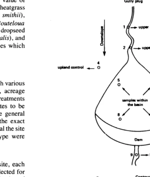
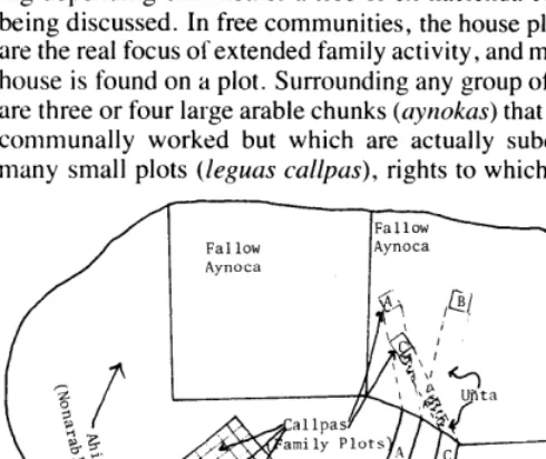
The original experimental trials consisted of grazing six !60-acre pastures during the spring or fall. In 1960 the original design was altered by dividing the !60-acre pastures in two and grazing six pastures during the spring or fall and six during the spring and fall (Fig. I). Cattle were placed in each pasture in sufficient numbers to achieve three expected levels of total utilization-light (50% utili- zation), moderate (65% utilization), or heavy (80% uti!ization)- which were generally different from the actual level of utilization which occurred. These trials continued through the 1970 grazing season, when the experiment was altered. Forage production and utilization were measured starting in 1955 and have been the basis for a number of studies conducted by personnel at the University of Idaho. Yearling cattle used during the experiment were supplied by local ranchers and were weighed on and off the pastures involved. Thus, a relatively complete data set was available that measured how alternative utilization patterns affected animal grazing, forage pro- duction, and other ecological parameters.

Records available from the Burley District (BLM) indicated that the direct seeding costs (‘36.5 I per acre) were generally of the same order of magnitude as the seeding costs of other projects that were established in southern Idaho during this period (Caton and Beringer 1960). However, the Point Springs project also included considerable fencing and water developments (wells, pipelines, troughs, and pumps which made the total investment costs ($15.57 per acre) for this project higher than that of similar seedings established in this area.

BLM personnel estimated the carrying capacity of the area to be 27 acres per AUM before the project was initiated. They also estimated that animals grazing this area were gaining I .4 pounds per day. From this basic information, it was estimated (Godfrey and Sellassie 1978) that I .6 pounds of gain per acre would have been foregone during the deferment period (1953 and 1954). It was also assumed that the I .6 pounds of gain per acre would have been obtained if these seedings had not been established (after 1954).

I4ode rate Spring

Heavy Fall

10

Moderate Fall

c

‘;:::

Spring

Heavy Spring

Light Fall

20 03

Moderate Heavy Spring Fall

Light Fall

Results and Discussion

The preceding data provided the basis for a economic evaluation of the seedings at Point Springs. While most readers recognize that range improvements that are established for various reasons, the following analysis assumes that the Point Springs project, like most similar improvements that were established during the 1950’s, was established with the primary

purpose of increasing domestic animal production.

Table 1. Total discounted (6% discount rate) net revenue per acre, Point Springs Experimental Pastures, southern Idaho, 1955-1970.

Grazing system

(stocking rates Price per pound associated with

Rank season) 15@ 30$ 4%

-

r

2

65.18 130.35 195.53

Estimated Actual Returns 61.41 122.82 184.23

The benefits obtained as a result of establishing the Point Springs seeding were determined in the following manner. The amount of animal gain (weight of animals taken off a pasture minus their “in” weight) was measured directly. This gain was then divided by the number of acres in the pasture where the animals grazed. The I .6 pounds of gain per acre that was assumed would occur “without” the seeding was then sub- tracted from these gains. The difference represented the net gain .-with” the project. These net gains were then multiplied by various prices and discounted to the beginning of 1953 for comparison with the costs incurred to seed the area involved. For example, the gains for the Point Springs pasture (Pasture 03, Fig. I ), which was used heavily during the spring, yielded gains which had a present value of Sl30.35 per acre

3

4 5

59.72 119.45 179.17

57.92 115.85 173.77

6 7

52.10 104.19 156.29

50.09 100.18 150.27

39.96 79.93 119.89

8

Heavy spring Moderate spring,

moderate fall Moderate spring,

light fall Moderate spring Light spring,

light fall Light spring Moderate spring

heavy fall Light spring,

heavy fall Light spring,

moderate fall Moderate fall Light fall Heavy fall

36.72 73.45 110.17

9

IO *I 1 12

35.16 70.33 105.49

19.65 39.29 58.92

19.19 38.38 57.56

16.68 33.35 50.03

I

30$(0- 1.6) + 30$(0- 1.6) +30$(3?.4- 1.6)+ .,.:0$(56.3- 1.6) I (I .06)’ (I .06x’ (I .06):% (1.06)” when a 6% discount rate and 30 cents per pound of gain is assumed. This present value was greater than the investment costs incurred (S15.57 per acre). Present values for the other Point Springs pastures are found in Table 1. These data indicate that when a 6% discount rate and 30 cents per pound of gain are assumed, every grazing pattern (season and intensity) yielded net returns (present value of gains with the seedings minus the present value of gains without the seeding) that were grater cate that when a 6% discount rate and 30 cents per pound greater than the investment cost (‘315.57) incurred.” Large differences in net returns exist between the grazing patterns, however. For ex- ample, pastures which were grazed only during the fall had net returns that were less than half as large as pastures which were grazed to some degree during the spring. This pattern closely parallels the results reported earlier by Currie (1970) for Colorado. This also indicates that grazing crested wheatgrass during the spring is generally a necessary condition for high net returns in the form of livestock production.

those reported by other researchers (e.g., Cordingly and Kearl 1975; Stevens and Godfrey 1976; and Nielsen and Hinkely 1975), but they also indicate the pattern of utilization (season and intensity) can have a major impact on the returns obtained. The different utilization patterns that have been implicitly assumed (e.g., take half and leave half) by other researchers probably represent one of the major reasons why the returns reported have varied widely .

While the preceding analysis indicates that the Point Springs seedings yielded net returns that were greater” than the costs incurred, this analysis is not complete. The major reason why the returns reported above are not complete is the fact that these seedings are being used at the present time-i.e., benefits continued beyond 1970. A simulation model was therefore developed which estimated the effect of other patterns of utilization and ecological parameters on forage production. These simulated amounts of forage production were then used to evaluate what returns could have occurred under circumstances which were different from the actual gains which occurred at Point Springs.

The results in Table I not only indicate that grazing during the spring results in higher net returns than grazing in the fall, but that these net returns increase with the intensity of graz- ing--i.e., net returns from heavy spring grazing were greater than moderate spring, which were, in turn, greater than light spring grazing. Returns obtained from grazing pastures during the spring and fall, however, did not follow as consistent a pattern with respect to grazing intensity as was evident for pastures which were only grazed during spring or fall. Moderate spring grazing, when combined with fall grazing, generally resulted in net returns that were higher than most alternative grazing patterns. These results not only show that some of the returns obtained at Point Springs were as large or larger than

Simulated Returns

A uniform set of data concerning forage production, utili- zation, precipitation, animal response, and other parameters was collected for each Point Springs pasture for the 1957 through 1970 grazing seasons. This data set’ was used to estimate the following forage production equation:

Y= -6489.3-5.62 X,-5.1 X,+221.1 X:,+95.54 X,+48.3 X, (5.05) (4.76) (1.17) (4.92) (1.58)

+66.32 X,+33.67 X7- 1.81 X, where (5.25) (2.86) (1.23)

- __--

.’ The crltcrlon of positive net benefits (present value of net returns minus investment co\t\) I\ only one of several criteria that could ha\!e been used. The other criteria that are ottcn uxd include benefit-cost ratios and internal rates of return. Discussions of these crltcrla and their major strengths and weaknesse\ are found in numerous sources-e.g., hIcKcan (1958). Merewitz and Sosnich (1971). LaBaron (1963). Prest and Turvey

( IO05 1.

_~_-- _ ~__--

: Scnsiti\ity analysis was performed for cattle prices as low as 15~ per pound and for Lariou5 interest rates. Only in cases where the interest rate was greater than 9% and cattle price\ Net-e 15~~ did any (heavy fall) of the net returns become less than the initial costs. ’ Xlat~y \tatlstical problems were encountered in estimating forage production and animal

re\pon\e functions from the\e data. This report contains the equations that were judged to be the most acceptable. Readers desiring additional detail regarding theseestimations should \ce Godfrey and Sellasie (1978). f values for the regression coefficients are shown m parenthesis below the respective coefficient.

Y= total amount of forage produced per acre X,=spring utilization in percent for the previous year X,=fall utilization in percent for the previous year X,,=time=year minus 1900

X,= inches of precipitation, November through March X,=inches of precipitation in April

X,,=inches of precipitation in May and June X,=inches of precipitation, July through October X,=X, squared

Thus, for example, the predicted amount of forage produced in a pasture grazed at a 50% utilization rate in the spring and a 30% rate in the fall, with the average rainfall pattern for the Point Springs area in 1967, would be 5 15.98 pounds per acre-i.e., [-6489.3 - 5.62 (50) - 5.1 (30) + 221.1 (67) + 95.5-l (3.-c-l) + 48.3 (1.06) + 66.32 (3.86) + 33.67 (3.41) -

I .81 (67)“].

Some of the regression coefficients above were not statisti- cally significant at high levels of confidence. For example, variables X:%(1= 1. I 17) and X,(t= 1.23) were not significantly different from zero at a probability level of less than 90%. While there is no statistical reason why these time variables should be retained, they were needed to simulate production over time. Variables having high t values were the variables which were expected to explain most of the variation. These were generally the same variables, primarily precipitation, that have shown high significance by other researchers (e.g., Currie and Peter- son 1966; Sneva and Hyder 1962; and Sharp 1970). In the discussion that follows, precipitation during the periods indi- cated in the above forage production equation were assumed to be normal (mean values were used), utilization was allowed to vary, and

mated.

the resultant forage production over time was esti-

After the amount of forage that would be produced under the various simulated conditions was estimated, it was necessary to convert these amounts to animal production. This was accomp- lished by multiplying the applicable forage produced by the percent consumed. These forage consumption estimates were then multiplied by 7.5 if spring grazing occurred, and by 30 if fall grazing occurred.” This yielded the expected amount of gain per acre that would be obtained. The 1.6 pounds of gain per acre that was assumed would occur without the project was then subtracted from this simulated gain. The resultant net gain was then multiplied by various beef prices to obtain net revenue. These amounts were then discounted for comparison with investment costs. These simulated net returns are shown in Table 2.

Several interesting inferences are shown by the data in Table 3 ” First whenever an area was grazed during the spring, the _.

estimate& net returns were greater than investment costs in- curred. However, if crested wheatgrass is grazed only at low rates of utilization (e.g., 20%) during the fall, the benefits in terms of animal gain may not be as great as the investment costs incurred. Second, heavy utilization, as was expected, resulted in the shortest project life (project life was determined when the simulated forage production yielded the “without” production

” Kcadcrs should reahze that these result\ could be modltied if better estimates of forage productlon over time were available, and that the simulations Involve extrapolations. These extrapolations would probably yield longer project lives if il better estima- tmp equation was available. The project lives reported in Table 1, however, are nearly ;LS long a\ most other researchers have reported.

Table 2. Estimated present value of increased net gains per acre under assumed management conditions, 1955 through end of project life.

Percent Percent spring fall utilization utilization

(X,1 (X,1

Project life (years)*

Price per pound (6% discount rate)

15@ 3Oe 4%

80 60 40 60 40 40 20 20 20 20

0 0

0 24 92.90 185.80 278.70 0 26 86.15 172.30 258.45 0 27 68.20 136.40 204.60

20 24 76.60 153.20 229.80

20 26 65.05 130. IO 195.15

40 24 59.55 119.10 178.60

0 29 38.50 77.00 115.50

20 27 42.10 84.20 126.30

40 26 43.15 86.30 129.45

60 24 41.70 83.40 125.10

80 24 23.05 46.10 69.15

60 26 20.40 40.80 61.20

40 28 15.20 30.40 45.60

20 29 7.30 14.60 21.90

ProJcct Ilte plu\ lY5-1 equals the year when the torapc production I\ pedlcted toequal the “u Ithout” Ickel of productlon. The length ot ltte ot the\e seedings 14 probably under- c\tlmutcd t-11 the equation used.

of I .6 pounds of gain per acre). Third, even though heavy utilization resulted in the shortest project life, the increased gain and resultant net returns more than offset the shorter project life. Thus, crested wheatgrass stands which are not subject to soil erosion could be used at relatively heavy rates of utilization. When productivity decreases, they could be reseeded or rested, and subsequently used at a heavy rate again. This would result in a utilization pattern similar to short rotation cycles in forest management- i.e., graze the area heavily for a relatively short period of time, reseed it, and start another cycle, versus a pattern ofutilization involving a relatively low rate of utilization, which would extend the life of the project. Fourth, seeding an area to crested wheatgrass is a relatively beneficial expenditure of funds, from an animal production point of view, if these areas are grazed during the spring by yearling cattle,’ particularly if grazed at relatively high rates. Fifth, the manner in which a seeding is grazed has, perhaps, the largest impact on returns obtained.

Conclusions

Several major conclusions can be made from the above. These conclusions also agree, in general, with those recom- mended by Sharp ( 1970), but differ to some degree from the recommendations made by Currie (1970).

1. Investments made to establish the crested wheatgrass seedings at Point Springs were relatively beneficial from an animal production point of view.

2. Grazing crested wheatgrass during the spring is a neces- sary prerequisite to high net returns.

3. Heavy utilization resulted in the highest net returns. Thus, if an area can be grazed at a high rate without destroying the’ area’s integrity (e.g., soil erosion), this will result in the greatest net returns.

-C. Grazing at heavy rates during the spring was a somewhat superior utilization pattern to spring-fall utilization.

’ The high results obtamed may not be mdlcative of other types of operations (e.g., cowcalf). The high anrmal gains reported during the spring indicate that most livestock operators would find the types of seedings reported above to be profitable, nevertheless.

5. Spring only or spring-fall use was clearly superior to a fall only utilization pattern.

0. Utilization of crested wheatgrass results in relatively low net returns in the form of domestic animal production, if crazing only occurs during the fall.

3. Variations due to differences in the pattern of utilization may be a major reason why diversified results have been reported by researchers which have evaluated the costs and rtY urns of various range improvement practices.

Range managers must therefore carefully weigh the manage- mcnt practices they advocate if maximum gains are to be achieved. Grazing practices which emphasize plant production, M.ith little consideration of the impact on animal response, may not result in highest animal gains. This may be particularly true in cases where light utilization, which favors a long project life, WI-ws heavier utilization and a shorter period is advocated. In short. season of use, as well as intensity, makes a big difference in the returns that can be expected from range improvement in\ cstments.

Bibliography

Caton, D.D., and Christopher Beringer. 1960. Costs and benefits of reseeding rangelands in southeastern Idaho. Idaho Agr. Exp. Sta. Bull. 326. 31 p.

Currie, P.O., and B. Peterson. 1966. Using growing season precipitation to predict crested wheatgrass yields. J. Range Manage. 19:284-288.

Currie, Pat 0. 1970. Influence of spring, fall and spring-fall grazing on crested wheatgrass. J. Range Manage. 23: 103-109.

Godfrey, E. Bruce, and Ephraim Sellassie. 1978. The economic returns from seeding an area to crested wheatgrass: the Point Springs experiment. Idaho Agr. Exp. Sta. Bull. (in press).

Heady, Harold F. 1975. Rangeland Management. McGraw-Hill Book Co., New York. 460 p.

Kearl, W. Gordon, and Robert V. Cordingley. 1975. Costs and returns from reseeding plains ranges in Wyoming. J. Range Manage. 28: 437-442.

LeBaron, Allen. 1963. A discussion-the internal rate of return and decisions to improve range. In: Report No. 5 of the Committee on Economics of Range Use and Development, Western Agr. Econ. Res. Count. Laramie. p. 117-127.

McKean, Roland. 1958. Efficiency in Government through Systems Analysis. Wiley. New York. 336 p.

Merewitz, L., and Stephen Sosnick. 1971. The Budget’s New Clothes. Markham Publishing Co. St Paul. 660 p.

Neilsen, Darwin B., and Stan D. Hinckley. 1975. Economic and envi- ronmental impacts of sagebrush control in Utah’s rangelands-a review and analysis. Utah Agr. Exp. Sta. Res. Rep. No. 25. 27 p.

Nielsen, Darwin B. 1977. Economics of range improvements: a rancher’s handbook to economic decision-making. Utah Agr. Exp. Sta. Bull. 466. 52 P.

Pr&, A.R., and Ralph Turvey. 1975. Benefit cost analysis: a survey. Econ. J. 75(300): 683-735.

Sharp, Lee A. 1970. Suggested management programs for grazing crested wheatgrass. Forest and Wildl. and Range Exp. Sta. Bull. No. 4, Univ. of Idaho, Moscow. 19 p.

Sneva, F.A., and D.N. Hyder. 1962. Estimating herbage production on semi- arid range in the intermountain region. J. Range Manage. 15: 88-93.

Stevens, Joe B., and E. Bruce Godfrey. 1976. An economic analysis of public range investments on the Vale project, 1960-69. Oregon Agr. Exp. Sta. Circ. of inform. 653. 19 p.

St&dart, Lawrence A., Arthur D. Smith, and Thadis W. Box. 1975. Range Management. McGraw-Hill, New York. 532 p.

FOR INFORMATION

WRITE:

Dept. EA.

University Microfilms International

300 North ZeebRoad

18

Bedford Row

Ann Arbor, Mich. 48106

London, WClR 4EJ

USA.

England

Seasonal Food Habits of White-tailed Deer

in the South Texas Plains

LEROY A. ARNOLD, JR. AND D. LYNN DRAWE

Abstract

From October 1972, through September 1974, rumen analyses were used to determine food habits of white-tailed deer on the H.B. Zachry Randado Ranch in south Texas. Sixty-nine plant taxa were identified in the diet. Year-round preferences for various forage classes were 21 .l% cactus, 32.7% browse, 26.6% forbs, 8.3% grasses, and 11.3% unknown. Cactus was heavily selected from June through September, and was consumed less but still heavily during October through January. Highest forb consumption occurred during March, April, and May. Browse usually was an important part of the diet, and grass consumption on untreated range was constantly low. A direct relationship was found between frequency with which a plant species was eaten and variability in the amount of that species consumed. Perennial plant species were more important as forage than annual species. Application of 2, 4-D herbicide caused grass consumption to increase 30 times over nonsprayed areas.

The increasing economic potential of white-tailed deer on private lands in Texas indicates a need for more detailed information about deer habitat requirements. Especially needed is information on the amounts of forage deer require and kinds they prefer, the seasonality of their feeding habits, and the effects on deer foods following control of rangeland vegetation. Identifying desirable deer forage could be of primary impor- tance in land-use planning that is compatible with production of quality deer.

Everitt (1972) indicated that the feeding habits of white- tails vary widely from herd to herd and often change with season of the year. Differences in ecological types, plant associations, land use, and density of deer populations account for many variations reported between herds (Korschgen 1962). This has

been verified in local studies by Halloran ( 1943), Davis ( 195 1 ), McMahan ( 1964)) Chamrad and Box ( 1968), Kelly ( 1970), and Everitt (1972). Seasonal variations in diet have been linked to changes in abundance, phenology , and nutrient quality of range plants during the year (Short 1971).

The tendency of deer diets to be highly localized puts a greater demand on landowners to establish individual manage- ment programs. This demand also is increased by the fact that in Texas access to game ranges is controlled by landowners. Controlled access, for all practical purposes, has put game animals in custody of the landowner instead of the state (Teer and Forrest 1968). This situation theoretically should allow the

greatest income from deer to be gained by ranches with good deer management.

This paper reports results of a study of seasonal food habits of white-tailed deer on the H.B. Zachry Randado Ranch in the western portion of the South Texas Plains. This study was conducted in an effort to expand on spring feeding habits examined by Everitt ( 1972). Objectives of this study were: ( 1) to

determine and compare seasonal food preferences of white- tailed deer on the ranch, (2) to establish a relative importance rating of foods eaten by deer on the ranch, and (3) to make recommendations for improved management of the deer herd based on food habits on this ranch and the surrounding area.

Study Area

The H.B. Zachry Randado Ranch consists of 3,045 ha in Jim Hogg and Zapata Counties in the South Texas Plains vegetational region (Gould 1975). It consists of rolling brushland intersected by gravel hills and gulleys. Eight soil types and six range sites lie within the ranch. The major portion of the ranch is a sandy loam site made up of fine sandy loam and loam soil types (Higginbotham 1975). Most sites on the ranch have been placed in fair range condition (Higginbotham

1975).

Both mechanical and chemical vegetation control have been practiced on the ranch. Approximately 810 ha were sprayed with 2,4,5-T during the spring of 1969 and 1970 primarily to control honey mesquite (Prosopis glandulosa). A large portion of this same area was sprayed with 2,4-D in April to control goldenweed (Isocoma corono- puolia). Also, areas of the ranch have been rootplowed or bulldozed and terraced in strips and patterns. The mosaic pattern of the several range sites and different control measures make vegetation of the ranch very diverse.

During the study approximately 200 head of cows and calves were managed on a one-herd, three-pasture, prescription grazing system. Deer had free access to the entire ranch, but movement off the ranch is limited by a 2.44-m “deer-proof” fence. The population of mature white-tailed deer on the ranch fluctuates around 400 animals annually. There is approximately a 1 to 1 buck:doe ratio as determined by helicopter census annually.

Methods

Food habits were determined by rumen analysis of 73 deer collected from October 1972 through September 1974. One to nine deer were collected monthly. Of these deer, 11 were bucks and 61 were does. After a deer was killed, the entire rumen contents were removed. A 0.95-liter randomly selected sample of solid matter was mixed with 10% formalin solution and placed in a plastic container. Strained samples, randomly selected from throughout the contents remaining on a #20 sieve, were analyzed by the point-frame method described by Chamrad and Box (1964) and Chamrad (1966).

Individual plant parts were identified to species and ordered into five classes: (1) cactus, (2) browse, (3) forbs, (4) grasses, and (5)

unknown material. Though cacti usually are reported as part of the browse class, it became apparent in this study, as well as the previous food habits study by Everitt (1972), that cacti are a highly important part of the diet on this ranch. Thus the Cactaceae have been considered separately.

Table 1. Ranking of the top 40 species found in deer diets on the H.B. Zachry Randado Ranch, 1972 to 1974, based on preference value Percent Frequency x Percent Volume).

Each species found in the diet was ranked by its preference value: percent frequency of occurrence multiplied by percent volume in the diet over 2 years (Chamrad and Box 1968).

Taxon

% Frequency

% Volume

Preference value’

Part of the ranch was sprayed with 2,4-D in April 1974, to control goldenweed. Rumen contents of four deer killed in the sprayed area were compared to rumen contents of eight deer killed on nonsprayed areas to determine if the application of 2,4-D had changed deer diet.

Data were transformed according to Ostle (1966) to correct for inherent bias in the raw data recorded as percentages. One-way analysis of variance was used to determine if statistical differences existed among months and selected groupings of sequential months for each plant class. By using all possible sequential monthly groupings, (i.e., 2 months, 3 months, etc.), it was possible to determine statistically which plant class was preferred and how long that class was preferred over another. Scheffe’s multiple contrast test for lack of fit was used to analyze the relationship between frequency of specific plants occurring in the diet and the variance with which they occurred (Steel and Torrie 1960).

Results and Discussion

Overall Food Preferences

Based on rumen analysis of 63 white-tailed deer collected outside the sprayed area, year-round preferences for various forage classes were 2 1.2% cactus, 32.7% browse, 26.6% forbs, 8.3% grasses, and 1 1.3% unknown material. The diet consisted of 69 identifiable plant taxa. There were 2 cacti, 32 browse, 34 forb, and 1 grass species identified in the year-round diet.

Pricklypear cactus (Opuntia lindheimeri) had the highest percent volume and frequency of any single species found in the diet (Table 1). It comprised 20.9% volume of the diet and had a frequency of 70.1%. It was the only species of cactus other than tasajillo (Opuntia leptocaulis) eaten by these deer. After de- leting deer that did not consume cactus, deer that consumed pricklypear had an average of 29.8% volume in their diet.

The second most heavily preferred species, a forb, was perennial lazy daisy (Aphunostephus riddeffii), which had an average volume of 6.5% and a frequency of 43.3%. Other species found to be heavily preferred, having a frequency of over 20%, were annual lazy daisy (A. kidderi), la coma

(Burnelia celustrina), granjeno (Ceftis pallida), prostrate euphorbia (Euphorbia prostrata), desert lantana (Lantana mucropodu var. ulbijloru), and honey mesquite (Table 1).

Deer on the ranch can best be described as browsing animals

Opuntis lindheimeri 70.1 20.9 1,463.g

Aphunostephus riddellii 43.3 6.5 279.6

Prosopus glandulosa 26.9 5.8 156.9

Aphunostephus kidderi 25.4 6.1 154.8

Bumelia celastrina 22.4 3.4 75.7

Celtis pullida 23.9 3.0 71.6

Commelina erecta 17.9 2.5 52.5

Acacia greggii 14.9 3.5 45.1

Lantuna macropoda var. albijlora 20.9 2.1 43.0

Zunthoxylum jagara 16.4 2.2 36.8

Porlieria angustijolia 28.4 1.2 32.9

Castela texana 17.9 1.6 27.9

Leucophyllum jrutescens 17.9 1.2 21.7

Euphorbia prostrata 20.9 1.0 21.3

Colubrinu texensis 14.9 1.3 19.1

Schue#eria cuneijolia 14.9 1.1 16.1

Xunthisma texanum 10.4 1.3 14.0

Physalis viscosa 11.9 0.9 11.1

Ambrosia psilostachya 11.9 0.9 10.7

Pithecellobium_flexicaule 7.5 1.3 9.5

Trisis rudiulis 8.9 1.1 9.4

Diospyros texana 9.0 1.0 9.0

Prosopis replans var. cinerascens 10.4 0.8 7.8

Menodora heterophylla 4.5 1.5 6.9

Cynanchum barbigerum 11.9 0.5 6.2

Ziziphus obtusijolia 10.4 0.5 5.3

Parthenium conjertum 8.9 0.5 5.0

Phorudendron sp . 5.9 0.5 3.1

Acuciu rigidula 7.5 0.4 2.8

Solanum triquetrum 5.9 0.4 2.7

Cocculus diversijolius 5.9 0.4 2.6

Psilostrophe gnaphlodes 4.5 0.5 2.1

Krumeria ramosissima 9.0 0.2 2.0

Ephedru antisyphilitica 6.0 0.2 1.4

Eysenhurdtia texana 6.0 0.2 1.3

Rutibidu columnaris 3.0 0.4 1.3

Opuntiu leptocaulis 6.0 0.2 1.3

Acleisanthes obtusa 4.5 0.3 1.1

Gauru brachycarpu 1.5 0.7 1.0

Zexmeniu hispida 4.5 0.2 0.8

’ L’alucs may not calculate: exactly because of rounding-oft.

and cactus consumption was found in this study, but there was an indication that it is eaten heavily during periods of high temperature.

when cactus is added to this class. Cactus and browse species combined made up approximately 53.8% volume of the diet on a year-round basis.

Cactus Consumption

Cactus consumption could not be linked directly to the availability of other plants. Many plants for which deer showed high preference during spring remained available into the summer when cactus consumption increased. Mesquite beans were preferred when available, from June through September, but even then cactus was selected highly.

There were significant seasonal fluctuations in the consump- tion of cactus based on statistical analyses (Table 2). The most significant change in cactus consumption of the monthly groupings tested was the 4-month grouping beginning in February. Cactus was heavily selected during June through September, making up 32.9% volume of the diet. It was selected less but still heavily during October through January, making up 26.7% volume of the diet. Minimal consumption of cactus occurred during February, March, April, and May, when it made up only 5 .O% volume of the diet.

Forbs, Browse and Grass Consumption

The pattern of forb consumption did not follow exactly the pattern found for cactus. There was an indication that the highest amounts of forbs are consumed when cactus is low in the diet (Table 2). Statistical analyses indicated the monthly group- ing which best demonstrates the forb consumption pattern would be the 3-month grouping beginning in March. Highest forb consumption occurred during March, April, and May, whereas the lowest was during September through February. Cactus, because of its low nutritive value, was classically Amounts of browse and grass in the diet remained relatively assumed a source of water for deer. No pattern between rainfall stable all year with no significant shifts in the amount consumed