1 1
Medium-range probabilistic forecasts of wind power
2
generation and ramps in Japan based on a hybrid ensemble
3
4
5
6
7
8
9
10
11
12
13
14
Masamichi Ohba, Shinji Kadokura, Daisuke Nohara
Environmental Science Research Laboratory,
Central Research Institute of Electric Power Industry
1646 Abiko, Abiko, Chiba, 270-1194, Japan
September 2018
15
16
Corresponding author: Masamichi Ohba
17
Central Research Institute of Electric Power Industry (CRIEPI)
18
Environmental Science Research Laboratory
19
1646 Abiko, Abiko, Chiba 270-1194, Japan
20
E-mail: [email protected]
21
22
2 ABSTRACT 23
24
This study shows the application of self-organizing maps (SOMs) to probabilistic 25
forecasts of wind power generation and ramps in Japan. SOMs are applied to atmospheric 26
variables obtained from atmospheric reanalysis over the region, thus deriving classified 27
weather patterns (WPs). Probabilistic relationships are established between the synoptic-28
scale atmospheric variables over East Japan and the generation of regionally integrated 29
wind power in East Japan. Medium-range probabilistic wind power predictions are 30
derived by SOM, as analog ensembles based on the WPs of the multi-center ensemble 31
forecasts. As this analog approach handles stochastic uncertainties effectively, 32
probabilistic wind power forecasts are rapidly generated from a very large number of 33
forecast ensembles. 34
The use of a multi-model ensemble provides better results than a one-forecast model. 35
The hybrid ensemble forecasts further improve the probabilistic predictability skill of 36
wind power generation, as compared with non-hybrid methods. It is expected that long-37
term wind forecasts will provide better guidance to transmission grid operators. The 38
advantage of this method is that it can include an interpretative analysis of meteorological 39
factors for variations in renewable energy. 40
41
Keywords: Self-organizing maps; Weather patterns; Synoptic circulation; Multi-model 42
ensemble; Wind power 43
3
1. Introduction
45
Wind energy is receiving increasing attention due to reasons ranging from climate 46
change to its status as the fastest growing energy source globally. Global production of 47
wind energy has significantly increased in recent decades [40]. Despite this rapid change, 48
wind energy technology is still considered imperfect. The main factor is the fluctuation 49
in wind energy production that can result in significant and rapid changes in power 50
generation over a short period, known as the “ramp” phenomenon [1]. As large-scale wind 51
energy ramp events lead to an increase in power grid instability, they must be balanced 52
by other power sources or storage systems, such as pumped-storage hydroelectricity. 53
Forecasting the timing of ramp events can help grid operators avoid unexpected electricity 54
imbalances. Even with the imminent need for ramp forecasts from power grid operators, 55
obtaining highly accurate ramp forecasts remains an important challenge from a practical 56
point of view. 57
Deterministic forecasting, based on numerical weather prediction, is one of the tools 58
that can provide useful information for decision-making by grid operators. However, 59
imperfect boundary conditions, initial conditions, and model formulation (e.g., dynamic 60
core, physics) result in nonlinear error propagation during model integration. To quantify 61
forecast uncertainty, more precise knowledge of the plausible future conditions is 62
required for decision-making. In recent decades, ensemble forecast techniques have been 63
developed as a tool for probability forecasting to generate a set of plausible future 64
atmospheric conditions. Medium-range (1 or 2 week) ensemble forecasts are a crucial 65
4
more time for preparation and decision-making than short-range (i.e., a few days) 67
forecasts. It is conceivable that probabilistic medium-range ensemble forecasts can be 68
useful to create weekly system operation plans of electric power and then increase the 69
capability of renewable energy ramps, adding value to power grid management by 70
providing more confidence (and less uncertainty) than deterministic forecasts. 71
In addition to ensemble methods, statistical post-processing is also necessary to 72
calibrate model output. Statistical/empirical post-processing techniques for numerical 73
weather forecasts are frequently-used, powerful approaches that improve the impacts of 74
model error or initial-boundary conditions. These techniques are now used in various end-75
user applications, including estimates of renewable energy production. A promising post-76
processing technique is the analog approach, in which, based on the assumption that if 77
forecasted current (synoptic) weather conditions are similar to that in the past, such as 78
spatial-time series of wind speed and direction, the local weather can be similar to that of 79
the past. Several studies have explored the use of analog-based methods for producing 80
both deterministic and probabilistic weather predictions [2,3,4,5,6,7]. Delle Monache et 81
al. [7] showed that the analog approach is useful only to calibrate raw numerical forecasts 82
and to generate probabilistic information from a purely deterministic forecast. Some 83
studies have discussed the application of an analog ensemble (AnEn) to regional 84
renewable energy forecasting [41,42]. 85
As a very large amount of forecast data is provided in medium-range ensemble 86
forecasts, efficient tools are required to extract useful information. The self-organizing 87
5
techniques, capable of projecting high-dimensional nonlinear features onto a visually 89
comprehensible two-dimensional map. Attempting to overcome the problem of 90
downscaling a large number of ensemble forecasts, recent studies [5,9,10,11] have 91
proposed the use of a SOM-based analog technique to estimate the local weather 92
condition from ensemble forecasts. However, no study has addressed the specific 93
application of using SOMs for medium-range wind power forecasts. 94
The goal of this study is to evaluate the ability of multi-model ensemble forecasts, 95
in combination with SOM-based analog methods, to forecast probabilities of area-96
integrated wind power and ramps for medium-range lead times. We applied SOMs to 97
analyzing an area for weather patterns (WPs) over East Japan, while using the analog 98
approach for ensemble forecasts to predict wind power generation for individual time 99
steps over the course of up to one week ahead. This method could be categorized as a 100
hybrid ensemble method, as suggested by Eckel and Delle Monache [19], that is skillful, 101
compared with that based on a single deterministic forecast. This hybrid ensemble 102
forecast (combined application of a multi-model ensemble and analog ensemble post-103
processing) offers relatively good prediction skill for wind power generation and its 104
climatological/meteorological interpretation. It is implied that the application of fast 105
techniques will increase decision-making capabilities in the user community, such as 106
electric power transmission system operators. This study is organized as follows. Section 107
2 provides a description of the dataset and the methods used in this study. Section 3 shows 108
6
multi-model ensemble in improving renewable energy predictability skill. Finally, 110
Section 4 provides a summary of the conclusions of this study. 111
112
2. Data and method
1132.1. Data
114
Three-hourly instantaneous values of atmospheric data for the period 1977–2010 were 115
obtained from the Japanese 55-year Reanalysis (JRA-55) [13].We used sea level pressure 116
(SLP) and surface wind at 10 m. These atmospheric variables were available at a 117
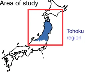
horizontal resolution of approximately 0.5°. This study focuses solely on integrated wind 118
power generation in the Tohoku region (blue region in Fig. 1), where the production of 119
wind-generated power is the highest in Japan. However, the time-window of wind power 120
observation is limited to only two years (FY2011/2012, i.e., April 2011 to March 2013). 121
In this study, we used the reconstructed wind power supply data from Ohba et al.[12], 122
from 1977 to 2010, for training our post-process model. This wind power data is 123
historically reconstructed using long-term observational data obtained from weather 124
stations in Japan, called the Automated Meteorological Data Acquisition System 125
(AMeDAS). In this study, a wind power variation that produces >30% change in wind 126
power generation over ≤ 6 h is defined as a “wind ramp event,” similar to previous study 127
[12]. The positive and negative quick change qualifies as a “ramp up and ramp down”, 128
respectively. 129
130
2.2 Ensemble forecasts
7
We also used past operational medium-range ensemble forecasts from five weather 132
prediction centers: JMA, NCEP, UKMO, CMC, and ECMWF. The ensemble forecast 133
data for 6-hourly values of sea level pressure and surface wind at 10 m are obtained from 134
the TIGGE (THORPEX Interactive Grand Global Ensemble) portal at ECMWF from 135
April 2011 to March 2013. As part of the THORPEX research program, this dataset is 136
currently available for non-commercial research purposes only at a two-day delay. The 137
forecast length used was 216 h, while the total ensemble size was 168. Only the ensemble 138
forecasts initialized at 12:00 UTC were used here to compare the products, while creating 139
a multi-model (i.e., multi-forecast center) ensemble based on the data from the five 140
weather prediction centers. 141
142
2.3 SOM technique
143
To establish links between various WPs and their impacts on regionally integrated 144
wind power, artificial neural network learning mechanisms were used in this study. SOMs, 145
developed by Kohonen [8], are one of the most commonly used nonlinear pattern 146
recognition techniques. SOMs project high-dimensional data to a visually 147
comprehensible two-dimensional map. Since SOMs provides a spatially organized set of 148
patterns of data variability, this technique has already been used in many synoptic 149
climatological analysis (readers can refer to Ohba et al. [14]). Patterns are topologically 150
ordered across the SOM array based on pattern similarity such that the farthest point of 151
the array contain patterns with the largest dissimilarity. As described in previous studies 152
8
In this study, we applied SOMs to the atmospheric variables derived from JRA55 154
around the Tohoku region (135°E-145°E, 35°N-44°N). The SOM projects these input 155
vectors onto regularly arranged two-dimensional arrays. Each of the arrays, referred to as 156
a node, has one reference vector. For example, a 50 × 50 grid SOM comprises 2500 157
reference vectors, which project onto a map composed of 2500 nodes. The reference 158
vector represents a generalized pattern of input vectors. For more details, refer to other 159
recent studies [11]. To train the SOM, we used SLP, surface wind vector, and surface 160
wind speed that showed high correlation to the wind power generation time series. We 161
used the torus-type SOM, instead of the conventional SOM, as it has no edges in the map 162
[16]. The SOM was applied on a three-month basis for the period 1977–2010, i.e., boreal 163
spring (March-April-May: MAM), summer (June-July-August: JJA), fall (September-164
October-November: SON), and winter (December-January-February: DJF). We mainly 165
present the winter results, during which high wind power generation are observed in Japan 166
[12]. 167
168
2.4 SOM based analog ensemble
169
A SOM is used in this study to estimate wind energy variation in the region by first 170
creating a relationship between atmospheric fields and local wind power generation. Each 171
node in SOM defines the wind power generation corresponding to each analog WP. Based 172
on this link between the SOM-obtained WPs (represented by reference vectors) and the 173
corresponding regionally integrated wind energy, we obtained a forecast PDF of wind 174
9
be regarded as an alternative to conventional analog [2,3] or analog-ensemble [7] 176
techniques presented in previous studies. While original analog-ensemble compare past 177
forecast with past forecast, this method compares past forecast with past analysis. The 178
SOM establishes a nonparametric relationship between predictor (WPs) and predictands 179
(wind power), subsequently requiring some statistical assumptions. In this study, the 180
forecast PDF is estimated using a set of past historical power generation data 181
corresponding to the best analogs (atmospheric reanalysis) for the current multi-model 182
ensemble forecast. The observational data for each analog is a member of the analog 183
ensemble [7]. One advantage may be to significantly lower the computational expense by 184
compressing the analogs using SOMs. While the original analog ensemble method[7,17] 185
generally uses a fixed number of analogs (such as 25 in [18]), the number of analogs (i.e., 186
number of best match) here are determined by the SOM, leading to a difference among 187
the SOM nodes in this method. To capture the spatial-time evolution of weather patterns, 188
±3 h time WP (i.e., 6 h time window for the analog trend) is also included in the input 189
vector, with all three WPs equally weighted. The predictor variables are also treated 190
equally. 191
To train the SOM, the same variables are extracted from the TIGGE ensemble data 192
for a particular region. Based on their distance from the reference vectors, each WP of 193
the ensemble forecasts is assigned to its best-match node. 168 forecast patterns are 194
available at 6-hour intervals. The ±3 h WPs for analog trends are obtained by linear 195
interpolation. Finally, the predicted composited PDF is obtained from the PDF, assigning 196
10
previous studies to provide greater detail in the atmospheric patterns relevant to wind 198
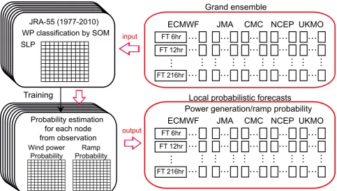
power variability. A schematic diagram of the algorithm of the downscaling technique is 199
shown in Fig. 2 and summarized below. 200
(1) Nine SOMs are applied to the atmospheric variables (top-left panel). 50 × 50, 201
80 × 80, 100 × 100 SOMs are used. Each SOM is trained separately with absolute 202
wind speed, wind vector, and SLP, i.e., a total of nine SOMs was used. 203
(2) PDFs of wind power generation and ramp probability are estimated (obtained 204
from observational data; bottom-left panel) for each node of (1). 205
(3) Using the SOMs obtained in (1), the node that best matches the output of the 206
multi-model ensemble forecasts (top-right panel) is selected from the SOM maps, 207
respectively. 208
(4) Wind power PDFs are derived by compositing the individual results of ensemble 209
forecasts obtained in (3) (bottom-right panel). 210
(5) The ensemble composited PDF of wind power generation for the targeted region 211
is obtained from (4). 212
The use of a 50 × 50 SOM results in a mean number of analogs of approximately 10, 213
but the 80 × 80 yielded about 4, and the 100 × 100 yielded about 2.5. We decided to use 214
three different SOM sizes since numbers of analog is important parameters of the analog 215
ensemble. This method could be regarded as a SOM-based hybrid multi-model analog 216
ensemble [11]. This analog ensemble is sensitive to the selection of parameters, such as 217
SOM dimension size and atmospheric variables. Sensitivity to the choice of input was 218
11
example, previous studies [18,17]on wind power generation suggest that wind speed and 220
direction are important for wind power forecasts. The selection of the variables in this 221
study is consistent with the results of previous studies. 222
223
3. Wind ramp prediction based on multi-model ensemble forecast
224
3.1. Estimated wind power and ramp
225
Generally, synoptic WPs, in relation to large-scale atmospheric conditions, are 226
important for comprehending wind power variations, since they affect near-surface wind 227
[20,21,22,23]. Therefore, they can be good predictors [24,25,26,27,28,39]. For example, 228
a frontal system passage, a low-level jet, and a planetary boundary layer growth can be 229
major factors in wind power variations [29]. Wind power ramps in Japan are mainly 230
caused by large fluctuations in wind speed in relation to the time-evolution of synoptic 231
circulation over East Asia [12] that always affects the load generation balance. 232
Since regional wind power variations can have various atmospheric origins, in 233
addition to being nonlinearly related to various meteorological factors, the classification 234
of synoptic-scale weather background conditions could be useful not only for 235
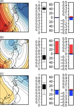
understanding weather factors, but also for improving wind power forecasts. First, in this 236
section, we present the results of a SOM-based WP classification. Three examples of WPs 237
are presented in Fig. 3. The mean atmospheric condition corresponds to the reference 238
vector derived from the 50 × 50 SOM analysis for SLP during DJF (i.e., the 3 h by 3 h 239
WPs, classified into 2500 nodes). The SOM analysis uses the 24480 (8 day-1 × 90 days in
240
12
removing the regional mean SLP values from the original data at each time step. Red and 242
blue shading indicate relatively high and low SLPs, respectively. We have also showed 243
the corresponding wind power generation, ramp up and down rates, and the node-mean 244
maximum increase and decrease in wind power generation over a period ≤ 6 h 245
corresponding with each WP. The patterns are selected as representative WPs that can 246
lead to relatively strong wind power generation or ramp, consistent with the dominant 247
wind power variation patterns in Japan, as discussed in previous studies [12]. 248
During winter, East Asian winter monsoons dominantly affect Japan’s climate and 249
local weather conditions, which is characterized by cold air outbreaks originating from 250
the negative zonal pressure gradients between the Aleutian Low and the Siberian High. 251
Two typical cyclone tracks are observed around Japan in winter, the southern coastal 252
cyclone track and the Japan Sea cyclone track. In Fig. 3, we see the impact of WPs on the 253
regional wind power generation. Corresponding to the distribution of SLP, the regional 254
wind power generation responses to the WPs are significantly different. For example, the 255
WP at the top of Fig. 3a, in eastern Japan, is covered by a strong zonal SLP gradient. The 256
SLP gradient is very effective at stably producing wind power over the region, with 257
variations ≤ 6 h being significantly weaker. However, low pressure systems approaching 258
the region from the northwest can cause more frequent ramp-ups (Fig. 3b). A meridional 259
SLP gradient covers the Tohoku region, associated with the low-pressure system located 260
at the north of the region (Fig. 3b), which can result in a rapid increase in surface wind 261
speeds within several hours. The cold front in relation to the mid-latitude cyclone passes 262
13
due to a reduction of high SLP over southwest Japan, resulting in more frequent ramp-264
downs. These results imply that different WPs can result in differences in wind power 265
generation and its subsequent stability. 266
An example of the relationships between WPs and wind power variations (node-267
mean) on the SOM lattice is presented in Fig. 4a. In this figure, a relatively strong wind 268
power generation (i.e., exceeding 0.7-0.8 p.u.) is observed in the bottom-right on the SOM. 269
We find strong contrast between nodes. This implies that integrated wind power 270
generation in this region is strongly dependent on synoptic WPs. The SOM analysis of 271
wind power variability over a 6 h time zone also allows us to estimate average wind power 272
variations. The occurrence rates of ramp-up and ramp-down events are also shown in Fig. 273
4a. It is clear that the nodes denoting a higher occurrence rate of ramp events are 274
separately concentrating in the SOM, implying that both, wind power generation and 275
ramps, are highly dependent on synoptic WPs. As denoted by Ohba et al. [12] many nodes 276
share probability of a ramp-up/down event. 277
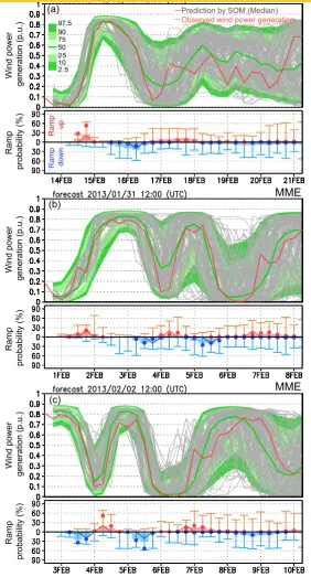
Figure 5 shows four examples of probabilistic forecasts of wind power generation 278
(top) and ramp (bottom), obtained from the multi-model ensembles (MME) of TIGGE 279
through SOM analysis. Gray lines represent the ensemble spread of the 50th percentile
280
output, obtained from the multi-model ensembles, while the green shading represents the 281
PDF of wind power generation, obtained from the hybrid (multi-model analog) ensemble 282
method. In these cases, throughout the period, the predicted wind power generation is in 283
close agreement with the observational result. The PDF covers the observed wind power 284
14
As for the second half of the period, the predicted wind power generation generally 286
captures the high risk of ramp events relatively well. As the best estimates (50th
287
percentile) of each ensemble member gradually extend, they approach the climatological 288
PDF with reductions in the day-to-day difference. 289
Probabilistic ramp forecasts are represented by red up) and blue (ramp-290
down) dots and bars in Fig. 5. The ramp probability obtained from the SOM node is 291
represented by a bar, which is the mean of the estimated value of 168 ensembles. The 292
error bar indicates the maximum and minimum values in the nine SOMs. We additionally 293
estimated the ramp probability using the 50th percentile value of each ensemble
294
(represented by the gray line in Fig. 5), denoted by a dot. The defined ramp-up and down 295
events seen in the observed wind power generation (i.e., actual ramp events) are 296
represented by red and blue lines. In these cases, ramp events are forecasted some number 297
of days before the occurrence. 298
Figure 4b shows the footprints of the multi-model ensembles on the SOM lattice 299
(Fig. 4a), predicted from 31 January 2013 (corresponding to Fig. 5b). The black line box 300
in Fig. 4b shows the actual WP seen in the SOM (i.e., the best-matching node of the 301
reanalysis). The frequency of occurrence of each SOM pattern results from mapping 168 302
ensembles × 4 times (in one day) to the SOM. If the forecasts are “perfect,” a very dark 303
square is identical to the solid black box, indicating that all forecast ensembles matched 304
the observations. The spread of the colored boxes indicates the range of skill of the 305
ensemble members, which varies by forecast days. The frequencies of WP in the multi-306
15
case, the multi-model ensemble forecast captures the atmospheric conditions of the actual 308
state relatively well for forecast day eight (except for forecast day four, which could be 309
related to an underestimation of rapid decrease in wind power in Fig. 5b). The expanse of 310
forecasts on the SOM can be an effective way to visually grasp the broadening of 311
ensembles and the reliability of prediction. 312
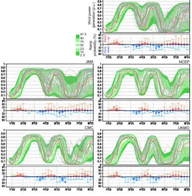
As an example of the inter-model difference, we also show the results of the individual 313
forecast centers separately in Fig. 6. We find a relatively large diversity of wind power 314
forecasts among the models. In this case, the UKMO model captures the ramp-up and 315
down that occurred on 4 February well. However, two days later, most of the models 316
capture both, the ramp-up (on 4 February) and down (on 5 February) well, as seen in Fig. 317
5c. In this case, the ensemble spread is relatively small in the UKMO and NCEP models. 318
319
3.2
Forecast skill of wind power variations
320
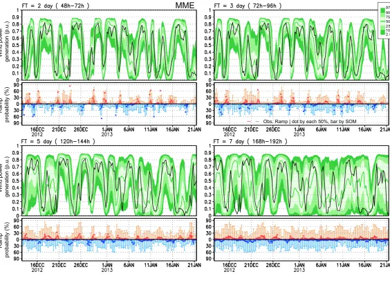
This subsection evaluates the predictability of wind power generations derived from 321
this method, based on the ensemble forecasts for FY2011/2012. Figure 7 shows the 322
forecasted PDF of wind power generation and ramp probability, obtained from the hybrid 323
multi-model-analog ensemble during mid-December to January of 2012/2013. The 324
forecasted PDF for each forecast day (2, 3, 5, and 7-day lead times) is shown separately. 325
The green shading in this Fig. shows the obtained PDF of the wind power generation, 326
while the dot at the bottom indicates the ramp probability. Moreover, the ramp probability 327
obtained from the ensemble means of SOM nodes are represented by the dots and bars. 328
16
region, the predicted wind power generation by the hybrid ensemble is relatively accurate 330
(i.e., most of the observed wind power generation is included in the 95th percentile),
331
especially for forecast day 2. The forecast skill decreases gradually, while the extent of 332
the PDF increases with respect to the forecast length, which could be regarded as a 333
convergence of the PDF towards the climatological PDF. The forecast uncertainty varies 334
substantially from day to day after forecast day 3. As for the longer range (forecast day 335
7), we find wide variations in the predictability/uncertainty, which is known as windows 336
for “forecasts of opportunity” [30,31,32,33] in relation to planetary-scale teleconnections. 337
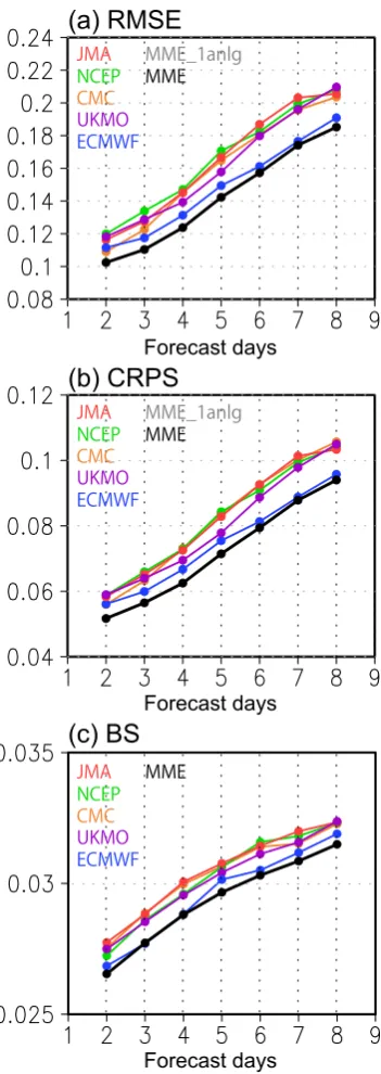
We have shown the root mean square error (RMSE) for each ensemble forecast 338
between the median of the probabilistic forecast and observations (Fig. 8a) to measure 339
the average forecast error. The ensemble forecast aims to construct the uncertainty 340
information. As a metric of probabilistic forecast verification, we have also included the 341
continuous ranked probability score (CRPS) [34], one of the measures of integrated 342
squared difference of the cumulative distribution function (CDF) of the forecasts (Fig. 343
8b) from observations. CRPS is commonly used to assess the respective accuracy of 344
probabilistic forecasts. The RMSE and CRPS of the wind power forecasts are shown for 345
the multi-model and each 5 ensemble forecasts for 2-8 days’ lead time. The results of 346
CRPS and RMSE are relatively similar to each other. Both, CRPS and RMSE, show that 347
the ECMWF ensemble forecasts have the best skill in the five models, while the UKMO 348
has the second-best skill. The remaining models have a similar level of accuracy. The 349
effect of combining the single-model systems can be seen in MME. The RMSE and CRPS 350
17
In addition to the forecasts of wind power generation, we also assessed the forecast 352
of wind ramp events provided from the hybrid ensemble forecasts in probabilistic form. 353
Commonly used verification methods for probabilistic forecasts are Brier score (BS) and 354
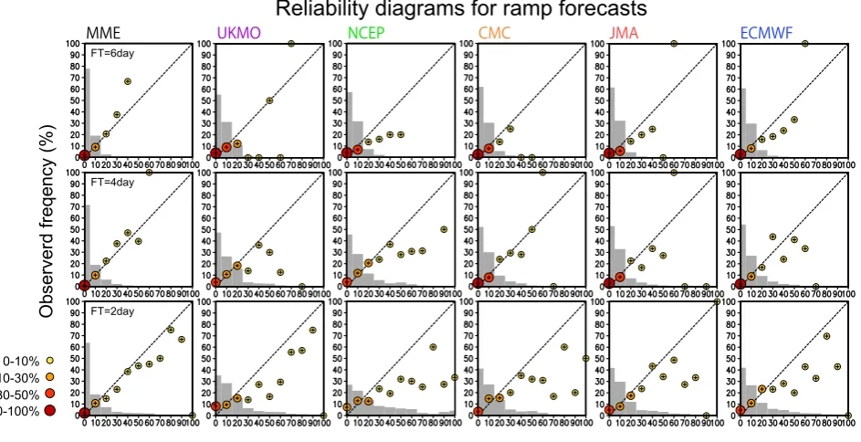
reliability diagrams. To check the skill of the wind power forecasts, we used BS (Fig. 8c) 355
and reliability diagrams obtained from the multi- and single-center ensembles for 356
FY2011/2012. Figure 9 presents the reliability diagrams for probabilistic forecasts of 357
wind power ramps over the region for that period. The centers of circles in the upper-left 358
and lower-right of the diagonal line indicate underestimation and overestimation of the 359
risks, respectively. Most of the single-center ensemble forecasts tend to overestimate the 360
risks, even with a lead forecast time of two days. The MME forecasts are significantly 361
more reliable than the other weather center’s ensembles for most lead times. The BS 362
shows that the ECMWF has the best, while the UKMO has the second-best performance. 363
From the BS and slopes of the reliability diagrams, the multi-model ensemble 364
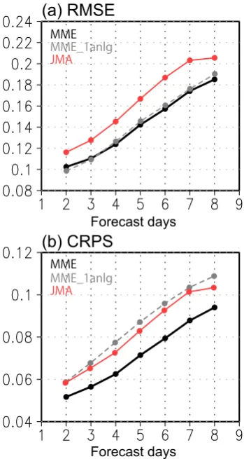
shows relatively good skill compared to the single-center ensemble forecasts for almost 365
all lead times. The construction of multi-model ensembles can improve reliability 366
throughout the forecast periods. The MME plots nearly diagonally at lead times of two to 367
four days, while showing improved forecast skill for the ramp events for all lead times 368
compared with the single model. 369
The improvement in wind ramp forecasts using the multi-model ensemble can be 370
attributed to the increase in ensemble spread. A particular single-center forecast cannot 371
always show the best performance in predicting ramp events, since the ensemble forecasts 372
18
ramp events, the other single-center ensemble forecasts do not necessarily show similarly 374
high probabilities. In this case, the MME will result in low probabilities of occurrence. 375
However, if most of the models are in good agreement regarding the occurrence of ramp 376
events, it can lead to the improvement of reliability with high forecast probabilities. 377
In addition to the effect of multi-model ensemble, we have also shown the effect of the 378
analog ensemble. The results of the single ensemble method for the JMA ensemble 379
forecasts and single-control forecast are presented in Fig. 10. To evaluate the skill of the 380
hybrid ensemble forecasts, we have also shown the forecast skill obtained from the 381
conventional (non-hybrid) scheme, namely, the nearest-neighbor single analog method. 382
The single analog method was carried out for comparing the results obtained from only 383
one single analog dataset (MME 1 analog). Instead of the use of SOM method, MME 1 384
analog predicted by picking up the reconstructed wind power data corresponding with the 385
highest similarity in the atmospheric variables among the reanalysis data. We used 386
Euclidean distance to measure similarity of the weather pattern and pick up one WP 387
presenting the highest similarity. We compared the results obtained from the MME 1 388
analog for the JMA forecast and the full MME. 389
The resulting RMSE increases with increasing forecast lead time for all approaches, 390
as shown in Fig. 10a. We see a relative improvement in RMSE when using the multi-391
model ensembles. Interestingly, the difference in RMSE of the median between the SOM 392
analog ensemble and the single ensemble is very small. This seems to be related to a 393
decrease in the number of valid analogs near the outer edge of the weather attractor. 394
19
Compared to RMSE, the prediction accuracy tends to be better in the analog ensemble 396
method in CRPS (Fig. 10b). Despite the decrease in computational cost, the SOM-based 397
analog ensemble method improves the skill versus conventional methods. This change 398
could be attribute to the effect of the analog ensemble, which makes a more realistic 399
forecasted PDF by obtaining nearby sample points. 400
401
4. Discussion and conclusions
402
In addition to evaluating the wind power potential [35], forecasting the variability of 403
wind power is one of most important challenges in the energy sector [1]. In this study, we 404
present the application of a SOM-based analog ensemble method for medium-range wind 405
power generation/variation forecasts by using multi-center ensemble forecast data, to 406
support system operation for transmission grid operators. As discussed in a previous study 407
of wind power and climate in Japan [12], the wind ramp events in East Japan are largely 408
affected by synoptic circulation. Most ramp-up events in Japan are due to approaching 409
extra-tropical cyclones, while most ramp-downs are due to reduced gradients of surface 410
pressure corresponding to the cover of anticyclonic highs. The complex relationships 411
between synoptic-scale WPs and regionally integrated wind power generation were 412
studied to obtain synoptic scale weather information around Japan by SOMs. We have 413
shown the applications of the SOM, not only for analyzing multi-model ensemble 414
forecasts, but also for the probabilistic forecasting of wind power generation and ramp 415
events. The skill of the wind power forecasts based on the hybrid multi-model analog 416
20
the results, we showed that regionally-integrated wind power production and variability, 418
in relation to synoptic-scale WPs, can be predicted days in advance. The medium-range 419
wind power forecast over Japan is relatively skillful. The skill predictability of multi-420
center ensembles improves that of single-center ensembles significantly when using the 421
perfect prognosis approach. We confirmed that the SOM-compressed analog ensemble 422
improves the forecasts and can then be an effective estimation method when a very large 423
number of ensemble members (i.e., multi-center ensemble) and historical local data are 424
used. The information obtained about predictive uncertainty can be fruitful as an 425
information source for decision-making in transmission grid operation. 426
The multi-model ensemble surpasses that of the single-model for both deterministic 427
and probability forecasts [36]. As the multi-center ensemble cancels individual systematic 428
errors in each model, it can provide more realistic estimates than individual forecast 429
systems [37,38]. Since the hybrid ensemble method presented in this study needs SOM 430
analysis in advance, it is computationally expensive and complicated method. However, 431
this method can be an alternative method when we cannot use long-term wind power data. 432
The hybrid ensemble method presented in this study have a potential to provide more 433
realistic PDF. Moreover, it can be employed rapidly, with a very large number of 434
ensemble forecasts outputs from medium-range (weekly) to long-range (seasonal). While 435
it cannot include various feedback processes at a local scale, our method is particularly 436
advantageous from a computational cost perspective, as it quickly provides a first-order 437
estimation of weather impacts on regional wind power resources. 438
21
Acknowledgements
440
This research was supported by the “Research and development projects on power 441
system output fluctuation-related technology” of the New Energy and Industrial 442
Technology Development Organization (NEDO). The authors express their gratitude to 443
the Ogimoto Lab at the Institute of Industrial Science, the University of Tokyo for 444
providing the observed area-integrated wind power generation data, derived from a 445
collaborative research project between the lab and the Japan Wind Power Association 446
(JWPA). Part of this work was supported by the JSPS KAKENHI Grant Number JP 447
17K18426. 448
22
References
450
1. Marquis, M.; Wilczak, J.; Ahlstrom, M.; Sharp, J.; Stern, A.; Smith, J.C.; Calvert, S. 451
Forecasting the wind to reach significant penetration levels of wind energy. Bull.
452
Amer Meteor Soc. 2011, 92, 1159–1171. 453
2. Lorenz, E.N. Atmospheric predictability as revealed by naturally occurring analogs. 454
J Atmos Sci. 1969, 26, 639–646. 455
3. Zorita, E.; von Storch, H. The analog method as a simple statistical downscaling 456
technique: comparison with more complicated methods. J. Clim. 1999, 12, 2474– 457
2489. 458
4. Timbal, B.; McAvaney, B.J. An analogue-based method to downscale surface air 459
temperature: application for Australia. Clim. Dyn.. 2001, 17, 947–963. 460
5. Gutierrez, J.M.; Cofino, A.S.; Cano, R.; Sordo, C. Analysis and downscaling multi-461
model seasonal forecasts in Peru using self-organizing maps. Tellus A.2005, 57, 435– 462
447. 463
6. Garcia-Morales, M.B.; Dubus, L. Forecasting precipitation for hydroelectric power 464
management: how to exploit GCM’s seasonal ensemble forecasts. Int J Climatol. 465
2007, 27, 1691–1705. 466
7. Delle Monache, L.; Eckel, T.; Rife, D.; Nagarajan, B. Probabilistic weather 467
23
8. Kohonen, T. Self-organized formation of topologically correct feature maps. 469
BiologicalCybernetics. 1982, 43, 59–69. 470
9. Hewitson, B.C.; Crane, R.G. Consensus between GCM climate change projections 471
with empirical downscaling: precipitation downscaling over South Africa. Int J
472
Climatol. 2006, 26, 1315–1337. 473
10. Borah, N.; Sahai, A.K.; Chattopadhyay, R.; Joseph, S.; Abhilash, S. et al. Self-474
organizing map-based ensemble forecast system for extended range prediction of 475
active/break cycles of Indian summer monsoon. J Geophy Res Atmos. 2013, 118, 1– 476
13. 477
11. Ohba, M.; Nohara, D.; Kadokura, S.; Toyoda, Y. Rainfall Downscaling of Weekly 478
Ensemble Forecasts using Self-Organizing Maps. Tellus A. 2016, 68, 29293. doi: 479
10.3402/tellusa.v68.29293. 480
12. Ohba, M.; Nohara, D.; Kadokura, S. Impacts of Synoptic Circulation Patterns on 481
Wind Power Ramp Events in East Japan. Renewable Energy. 2016, 96, 591–602. 482
13. Kobayashi, S.; Ota, Y.; Harada, Y.; Ebita, A.; Moriya, M.; Onoda, H. et al. The JRA-483
55 Reanalysis: General specifications and basic characteristics. J Meteor Soc Japan
484
2015, 93, 5–48. 485
14. Ohba. M.; Kadokura, S.; Nohara, D.; Toyoda, Y. Anomalous Weather Patterns in 486
Relation to Heavy Precipitation Events in Japan during the Baiu Season. Journal of
487
24
15. Reusch, D.B.; Alley, R.B.; Hewitson, B.C. North Atlantic climate variability from a 489
self-organizing map perspective. J Geophys Res. 2007, 112, D02104. doi: 490
10.1029/2006JD007460. 491
16. Ito, M.; Miyoshi, T.; Masuyama, H. The characteristics of the torus self-organizing 492
map. Proc 16th Fuzzy System Symp Akita Japan Society for Fuzzy and Systems 2000, 493
373–374. 494
17. Alessandrini, S.; Delle Monache, L.; Sperati, S.; Nissen, J. Short-term wind power 495
forecasting with an analog ensemble. Renewable Energy. 2015, 76, 768–781. 496
18. Vanvyve, E.; Delle Monache, L.; Monaghan, A.J.; Pinto, J. Wind resource estimates 497
with an analog ensemble approach. Renewable Energy. 2015, 74, 761–773. 498
19. Eckel, F.A.; Delle Monache, L. A hybrid NWP-analog ensemble. Monthly Weather
499
Review. 2016, 144, 897–911. 500
20. Klink, K. Atmospheric circulation effects on wind speed variability at turbine height. 501
J Appl Meteorol Climatol. 2007, 46, 445–456. 502
21. Cutler, N.J.; Outhred, H.R.; MacGill, I.F.; Kepert, J.D. Predicting and presenting 503
plausible future scenarios of wind power production from numerical weather 504
prediction systems: a qualitative ex ante evaluation for decision making. Wind Energy
505
2012, 15, 473–488. 506
22. Hamlington, B.D.; Hamlington, P.E.; Collins, S.G.; Alexander, S.R.; Kim, K.Y. 507
25
Geophys Res Lett. 2015, 42, 145–152. 509
23. Gibson, P.B.; Cullen, N.J. Synoptic and sub-synoptic circulation effects on wind 510
resource variability – A case study from a coastal terrain setting in New Zealand. 511
Renewable Energy. 2015, 78, 253-263, doi:10.1016/j.renene.2015.01.004. 512
24. Pryor, S.C.; Schoof, J.; Barthelmie, R.J. The impact of non-stationarities in the 513
climate system on the definition of a 'normal wind year': A case study from the Baltic. 514
Int J Climatol. 2005, 25, 735–752. 515
25. Davy, R.; Milton, J.; Russel, C.; Coppin, P. Statistical downscaling of wind variability 516
from meteorological fields. Bound Layer Meteorol. 2010, 135, 165-175. 517
26. Peña, J.C.; Aran, M.; Cunillera, J.; Amaro, J. Atmospheric circulation patterns 518
associated with strong wind events in Catalonia. Nat. Hazards Earth Syst Sci. 2011, 519
11, 145–155. 520
27. Brayshaw, D.J.; Troccoli, A.; Fordham, R.; Methven, J. The impact of large scale 521
atmospheric circulation patterns on wind power generation and its potential 522
predictability: a case study over the UK. Renewable Energy. 2011, 36, 2087–2096. 523
28. Ely, C.R.; Brayshaw, D.J.; Methven, J.; Cox, J.; Pearce, P. Implications of the North 524
Atlantic Oscillation for a UK-Norway renewable power system. Energy Policy. 2013, 525
62, 1420–1427. 526
29. Deppe, A.J.; Gallus, W.A.; Takle, E.S. A WRF ensemble for improved wind speed 527
26
30. Marshall, A.G.; Hudson, D.; Hendon, H.H.; Pook, M.J.; Alves, O.; Wheeler, M.C. 529
Simulation and prediction of blocking in the Australian region and its influence on 530
intra-seasonal rainfall in POAMA-2. Clim Dyn. 2014, 42, 3271–3288. 531
31. Hudson, D.; Alves, O.; Hendon, H.H.; Marshall, A.G. Bridging the Gap between 532
Weather and Seasonal Forecasting: Intraseasonal Forecasting for Australia. Q J R
533
Meteor Soc. 2011, 137, 673–689. 534
32. White, C.J.; Hudson, D.; Alves, O. ENSO, the IOD and the intraseasonal prediction 535
of heat extremes across Australia using POAMA-2. Clim Dyn. 2014, 43, 1791–1810. 536
537
33. Johnson, N.C.; Collins, D.C.; Feldstein, S.B.; L'Heureux, M.L.; Riddle, E.E. Skillful 538
wintertime North American temperature forecasts out to four weeks based on the 539
state of ENSO and the MJO. Wea Forecasting. 2014, 29, 23–38. 540
34. Hersbach, H. Decomposition of the continuous ranked probability score for ensemble 541
prediction systems. Wea. Forecasting. 2000, 15, 559–570. 542
35. Archer, C.L.; Jacobson, M.Z. Evaluation of global wind power. J Geophys Res Atmos. 543
2005, 110, D12110. 544
36. Park, Y.Y.; Buizza, R.; Leutbecher, M. TIGGE: Preliminary results on comparing and 545
combining ensembles. Q J R Meteorol Soc. 2008, 134, 2051–2066. 546
37. Matsueda, M., Tanaka, H.L. Can MCGE outperform the ECMWF ensemble? SOLA. 547
27
38. Johnson, C.; Swinbank, R. Medium-range multimodel ensemble combination and 549
calibration. Q J Roy Meteorol Soc. 2009, 135, 777–794. 550
39. Gibson, P.B.; Cullen, N.J. Regional variability in New Zealand’s wind resource 551
linked to synoptic-scale circulation: implications for generation reliability. Journal
552
of Applied Meteorology and Climatology. 2015, 54, 944-958. 553
40. International Energy Agency World energy outlook: 2016. OECD/IEA. 2016, 684. 554
41. Junk, C.; Delle Monache, L.; Alessandrini, S.; von Bremen, L.; Cervone, G. 555
Predictor-weighting strategies for probabilistic wind power forecasting with an 556
analog ensemble. Meteorologische Zeitschrift. 2015, 24, 361-379. 557
42. Davò, F.; Alessandrini, S.; Sperati, S.; Delle Monache, L.; Airoldi, D.; Vespucci, M.T. 558
Post-processing techniques and principal component analysis for regional wind 559
28
List of Figures
561
562
Figure. 1. Area of study in East Japan (red solid box) used to define the atmospheric 563
patterns. The blue shading represents the Tohoku region (served by Tohoku 564
Electric Power Co., Inc.), Japan. 565
566
Figure. 2. Schematic of the hybrid ensemble using SOM. The multiple SOM 567
classifications of WP are based on the three atmospheric variables during 1977– 568
2011 (top, left). Based on the SOM lattices, the PDF of wind power generation 569
and ramp probability are estimated for each node (bottom, left). By using the SOM 570
lattice, the forecasted wind power generation and variation are obtained (bottom, 571
right) from the 168 members of the multi center ensemble forecasts (top, right). 572
573
Figure. 3. (a)–(c) Three examples of WPs (SLP) derived from the 50 × 50 SOM non-574
linear classification (hPa: red and blue shading). Right panels show the WP-575
related wind power generation (p.u. black error bar for 5th, 25th, 75th, and 95th
576
percentiles), frequency occurrence rate (%) of ramp-up (red) and down (blue), 577
and maximum up (red) and down (blue) of wind power generation (p.u.) over ≤ 578
6 hours for each SOM node. 579
580
Figure. 4. (a) The median values of wind power generation (left), frequency occurrence 581
29
Each bottom-left figure show the correspondence with Figs. 3a-c, respectively. 583
(b) SOM frequency (best-matched) of the 168 multi-center ensemble members 584
on the 50 x 50 SOM lattice for forecast days 1–8 initiated from 1st January 2013.
585
Solid black box represents the actual state. 586
587
Figure. 5. Forecasted 6-h wind power forecasts obtained from the single center ensembles 588
with SOM-based analog-ensemble, initiated from (a) 13th February 2012, (b) 1st
589
January 2013, and (c) 2nd February 2013, at 12:00 UTC, as examples of the
590
forecast results. Red line represents the observed wind power generation. PDFs 591
of wind power generation obtained from the hybrid ensemble are represented by 592
green shading. Gray line represents median values of each ensemble member 593
(total 168 lines). Each figure at the bottom shows the forecasted ramp probability 594
obtained from the SOM nodes and the medians of each ensemble are represented 595
by red and blue bars and dots, respectively, with the error bar. Observed ramp up 596
and ramp down events (actual state) are represented by the red and blue lines, 597
respectively. 598
599
Figure. 6. Same as Fig. 5, except it is obtained from the five single-center ensembles with 600
SOM-based analog-ensemble initiated from 1st January 2013, at 12:00 UTC.
601
602
Figure. 7. Forecasted 6-h wind power generation obtained from the hybrid ensemble for 603
2-day, 3-day, 5-day, and 7-day forecasts around 1st January 2013. Black line
30
represents the observed wind power generation. Forecasted PDFs of wind power 605
generation obtained from the hybrid ensemble are represented by green shading. 606
Each figure at the bottom shows the forecasted ramp probability obtained from 607
the SOM nodes and the medium of each ensemble, represented by red and blue 608
bars and dots, respectively. Observed ramp up and ramp down events (actual 609
state) are represented by the red and blue lines, respectively. 610
611
Figure. 8. (a) RMSE, (b) continuous ranked probability score, and (c) Brier score for wind 612
power generation forecasts by CMC (orange), ECMWF (blue), JMA (red), 613
NCEP (green), UKMO (purple), and MME (black) for the targeted region from 614
Apr 2011 to May 2013. 615
616
Figure. 9. Reliability diagrams for 2-day, 4-day, and 6-day forecasts of wind ramp events 617
in the Tohoku region from Apr 2011 to May 2013, obtained from the MME and 618
five single-center ensembles. Frequency histograms are represented by gray bars 619
and dot colors. 620
621
Figure. 10. Same as Fig.8a and 8b, except for wind power generation forecasts, using 622
single analog method for MME (gray). JMA (red) and MME (black) are the same 623
as in Fig. 8. 624
Area of study
Tohoku region
Fig. 1. Area of study in East Japan (red solid box) used to define the atmospheric patterns.
The blue shading represents the Tohoku region (served by Tohoku Electric
WP classification by SOM
Probability estimation for each node from observation Grand ensemble input output JRA-55 (1977-2010) Ramp Probability
Local probabilistic forecasts Training SLP Wind power Probability JMA ECMWF
FT 216hr
…
FT 6hr FT 12hr
…
…
…
…
CMC NCEP UKMO
…
…
…
…
…
…
…
…
…
…
…
…
…
…
…
…
…
…
…
…
JMA ECMWFFT 216hr
…
FT 6hr FT 12hr
…
…
…
…
CMC NCEP UKMO
…
…
…
…
…
…
…
…
…
…
…
…
…
…
…
…
…
…
…
…
Power generation/ramp probability
FIG. 2. Schematic diagram of the hybrid ensemble by using SOM. The multiple different
1
SOM classifications of the WP are based on the three atmospheric variables
2
during 1977-2011 (top left). Based on the SOM lattices, the PDF of wind power
3
generation and ramp probability are estimated for each node (bottom left). By
4
using the SOM lattice, the forecasted wind power generation and variation are
5
obtained (bottom right) from the 168 members of the multi center ensemble
6
forecasts (top right).
(a)
(b)
(c)
FIG. 3. (a)-(c) Three examples of WPs (SLP) derived from the 50 x 50 SOM non-linear
1
classification (hPa: red and blue shading). Right panels show the WP-related
2
wind power generation (p.u. black error bar for 5th, 25th, 75th and 95th percentiles),
3
frequency occurrence rate (%) of ramp-up (red) and down (blue), and maximum
4
up (red) and down (blue) of wind power generation (p.u.) over a period ≤ 6 hours
5
for each SOM node.
Wind power generation(a) Relationships between WPs and wind power variations on SOM Ramp up rate Ramp down rate
(b) Footprints of multi center grand ensembles on SOM
Fig. 4. (a) The median values of wind power generation (left), frequency occurrence rate
1
(%) of ramp-up (middle) and ramp-down (right) within each SOM node. Each
2
bottom-left figures show the correspondence with Fig. 3a-c, respectively. (b)
3
SOM frequency (best-matched) of the 168 multi-center ensemble members on
4
the 50 x 50 SOM lattice for forecast days 1–8 initiated from 1st January 2013.
5
Solid black box represents the actual state.
MME
MME
(b)
(c)
Wind power
generation (p.u.)
Ramp
probability (%)
Wind power
generation (p.u.)
Ramp
probability (%)
Wind power
generation (p.u.)
Ramp
probability (%)
Ramp up
Ramp down
2.5
FIG. 5. Forecasted 6-h wind power forecasts obtained from the single center ensembles
with SOM-based analog-ensemble initiated from (a) 13 February 2012, (b) 1
January 2013, and (c) 2 February 2013 12:00 UTC as examples of the forecast
results. Red line represents the observed wind power generation. PDFs of wind
power generation obtained from the hybrid ensemble are represented by green
shading. Each bottom figure shows the forecasted ramp probability obtained
from the SOM nodes (medium of each ensemble) are represented by red and blue
bars (dots) with the error bar. Observed ramp up and ramp down events (actual
JMA NCEP
UKMO CMC
generation (p.u.)
Ramp
probability (%)
97.5 90 75 50 25 10 2.5
Ramp up
Ramp down
FIG. 6. Same as Fig. 5 except for that is obtained from the five single-center ensembles
MME
Wind power
generation (p.u.)
Ramp
probability (%)
97.5 90 75 50 25 10 2.5
Wind power
generation (p.u.)
Ramp
probability (%)
- - Obs. Ramp | dot by each 50%, bar by SOM
FIG. 7. Forecasted 6-h wind power generation obtained from the hybrid ensemble for
2-1
day, 3-day, 5-day, and 7-day forecasts around 1 January 2013. Black line
2
represents the observed wind power generation. Forecasted PDFs of wind power
3
generation obtained from the hybrid ensemble are represented by green shading.
4
Each bottom figure shows the forecasted ramp probability obtained from the
5
SOM nodes (medium of each ensemble), represented by red and blue bars (dots).
6
Observed ramp up and ramp down events (actual state) is represented by the red
7
and blue lines, respectively.
Forecast days Forecast days
(a) RMSE
(b) CRPS
(c) BS
Forecast days
FIG. 8. (a) Root mean square error, (b) continuous ranked probability score, and (c) Brier
score for wind power generation forecasts by CMC (orange), ECMWF (blue),
JMA (red), NCEP (green), UKMO (purple), and MME (black) for the targeted
FT=2day FT=4day FT=6day
Reliability diagrams for ramp forecasts
Observerd freqency (%)
Forecast probability (%)
50-100% 0-10% 10-30% 30-50%
FIG. 9. Reliability diagrams for 2-day, 4-day, and 6-day forecasts of wind ramp events in
1
the Tohoku region from Apr 2011 to May 2013 obtained from the MME and five
2
single-center ensembles.
Forecast days Forecast days
(a) RMSE
(b) CRPS