Tanja Lange1, Christine van Vredendaal1,2, and Marnix Wakker2
1 Department of Mathematics and Computer Science Eindhoven University of Technology
P.O. Box 513, 5600 MB Eindhoven, The Netherlands
[email protected], [email protected]
2
Brightsight B.V.
Delftechpark 1, 2628 XJ Delft, The Netherlands
Abstract. Side-channel attacks are a powerful tool to discover the cryp-tographic secrets of a chip or other device but only too often do they require too many traces or leave too many possible keys to explore. In this paper we show that for side channel attacks on discrete-logarithm-based systems significantly more unknown bits can be handled by using Pollard’s kangaroo method: ifbbits are unknown then the attack runs in 2b/2 instead of 2b. If an attacker has many targets in the same group and thus has reasons to invest in precomputation, the costs can even be brought down to 2b/3.
Usually the separation between known and unknown keybits is not this clear cut – they are known with probabilities ranging between 100% and 0%. Enumeration and rank estimation of cryptographic keys based on partial information derived from cryptanalysis have become important tools for security evaluations. They make the line between a broken and secure device more clear and thus help security evaluators determine how high the security of a device is. For symmetric-key cryptography there has been some recent work on key enumeration and rank estimation, but for discrete-logarithm-based systems these algorithms fail because the subkeys are not independent and the algorithms cannot take advantage of the above-mentioned faster attacks. We present-enumeration as a new method to compute the rank of a key by using the probabilities together with (variations of) Pollard’s kangaroo algorithm and give experimental evidence.
Keywords: Side-channel attacks, template attacks, key enumeration, rank estimation, discrete logarithms, Pollard-kangaroo method, precom-putation
1
Introduction
In security evaluations it is important to investigate how well cryptographic implementations fare against side-channel attacks (SCA’s). Numerous of these
This work was supported by the Netherlands Organisation for Scientific Re-search (NWO) under grant 639.073.005. Permanent ID of this document:
attacks are known: In this paper we will be most interested in the Template Attacks introduced by Chari, Rao and Rohatgi [3]. These attacks are among the strongest possible attacks in the sense that they extract all possible information of the samplesS measured from a secret-key operation. They assume access to an identical device as used by the target and use it to produce precise multi-variate characterizations of the noise of encryptions with different keys. By a process of iterative classification they then attempt to derive the key used when measuringS. At each iteration a few bits are added to the templates. Each set of a few bits is called a subkey.
In [3] iterative classification was performed until only a few candidates for the key were left. We however accept being left with a larger number of possibilities of which we are 100% sure that they are the likeliest keys according to our at-tack results and then continue to enumerate the remaining keys. This might be faster than continuing to attack and hoping to get more significant results. The motivation for this approach is the guy in the security evaluation lab. He starts his template attack and if he were to spend a long enough time he might find the key. However if he is able to enumerate 2b keys, then the lab guy might as well stop the measurements after reducing the space of the remaining keys to an interval of size 2b. By pruning the space further he will only risk throwing out the actual key even though he could have enumerated it. Another motivation for our approach is that there are some implementations where it does not matter how long the guy stays in the lab, the power traces will not give away more information. In this case we will still have a (larger) space of possibilities we need to enumerate based on all the information we were able to get.
When we have the results of such a SCA we can take two approaches. The first is the black-box approach of key enumeration. A key enumeration algorithm takes the SCA results as input and return keyskin order of likelihood. The position of a k in such an ordering is called its rank r. For symmetric-key cryptogra-phy some research has been done on this subject. Pan, van Woudenberg, den Hartog and Witteman [10] described a sub-optimal enumeration method with low storage requirements and an optimal method that required more storage. Veyrat-Charvillon, G´erard, Renauld, and Standaert [17] improved the optimal algorithm to require less storage and be able to enumerate more keys faster. The second way of looking at a SCA result is the white-box approach of rank es-timation. This method is particularly relevant for security evaluation labs. Using modern technology it is feasible to enumerate 250 to 260 keys, but when a key is ranked higher, we can only say that its rank is higher than∼260 (the rank at which the memory is exceeded). For security evaluations of the encryption algorithm however more accuracy is required. A rank estimation algorithm is able to extract information about the rank rof k without enumerating all the keys. For symmetric cryptography like AES such an algorithm was put forth by Veyrat-Charvillion, G´erard and Standaert in [18].
Diffie-Hellman Key Exchange, k might be recovered by enumerating the most likely candidates. Contrary to the assumptions in the previously mentioned algorithms, the information on the subkeys is not independent for ECC and therefore we can-not use the existing algorithms. On the bright side, in ECC we are working with cyclic groups and we can use this structure to speed up enumeration. This way, enumeration can be interpreted as finding the solution to the Discrete Logarithm Problem (DLP) by using partial information on the subkeys. We present our own algorithm which utilizes Pollard’s kangaroo methods (see [11], [12], [5], [14], [16]) to enumerate with an error margin. In trade for this error margin we are able to enumerate a space of `keys inO(√`) group operations.
If we make use of a precomputation table like was proposed in [1] we can reduce the expense per key toO(√3
`) operations. This improvement of Pollard’s meth-ods lends itself particularly well to use in side-channel attacks. The creation of the precomputation table costsO(√3`2) group operations and a specific table can only be used to speed up solving of DLPs in one particular group and interval length. So creating the table is only useful if we want to perform an attack a lot of times on the same length interval of a certain subgroup, but this is a fairly common scenario since many smart card vendors implement the NIST P-256 curve for which the curve equation and the base point are standardized. This means that security evaluation labs can create the most commonly needed tables beforehand and re-use them every time an attack is performed on an implemen-tation for this curve.
We end this introduction with noting that even though the results in this paper are posed in the setting of elliptic curves, the techniques are applicable to solving a DLP in any cyclic group.
2
Background
This section gives a short description of methods to solve the Discrete Loga-rithm Problem (DLP) in a group of prime order n. The “square-root methods” solve this problem on average in O(√n) group operations. We will use additive notation since the main application is to is to solve the DLP on an elliptic curve
E over a finite fieldFp but the methods work in any group. Let P, Q∈E(Fp) be in a cyclic group; the goal is to find an integerksuch thatQ=kP.
2.1 A Short History of Discrete Logarithm Algorithms
A well known method is Shanks’ Baby-Step-Giant-Step (BSGS) method [13]. It uses a table to find collisions between baby steps 0P, P, . . . ,(m−1)P and giant stepsQ−0P, Q−mP, Q−2mP, Q−3mP, . . ., wherem≈√n. This finds
k=k0+k1mas the collision ofk0PandQ−k1mP inO(m) steps. A drawback of this method it that it has a storage requirement ofmelements, which is a more serious limitation thanO(m) computation. If the discrete logarithm kis known to lie in an interval [a, b] of length `then choosing m ≈√` gives a runtime of
The Pollard-ρ method [11] gives a solution to the storage problem. It uses a deterministic random walk on the group elements with the goal of ending up in a cycle (which can be detected by Floyd’s cycle finding algorithm). The walk is defined in such a way that the next step in the walk depends solely on the representation of the current point and that a collision on the walk reveals the discrete logarithm k. Van Oorschot and Wiener [16] introduced a parallel version of the Pollard-ρmethod which gives a linear speed-up in the number of processors used. They use distinguished points: a point is a distinguished point if its representation exhibits a certain bit pattern, e.g., has the top 20 bits equal to zero. Whenever one of the parallel random walks reaches such a point it is stored on a central processor. A collision between two of these distinguished points almost surely reveals the value of the key. This method is an improvement over BSGS in that the storage requirements are minimal, but the algorithm is probabilistic and it cannot be adapted to search an interval efficiently.
Pollard’s kangaroo method solves the latter problem. It reduces the storage to a constant and is devised to search for the solution of a DLP in an interval of length`. The mathematical ingredients, the algorithm and improvements are the topic of the remainder of this section.
2.2 Mathematical Aspects of Kangaroos
To adequately explain Pollard’s kangaroo method we first have to dive into the notion of a mathematical kangaroo. We define a kangaroo by the sequence of its positions Xi ∈ hPi. Its starting point is X0 = s0P for a certain starting values0 and the elements that follow are a pseudo-random walk. The steps (or rather jumps) of a kangaroo are additions with points from a finite set of group elementsS={s1P, . . . , sLP}.
The step sizessiare taken such that their average iss=β
√
`for some scalar
β. To select the next step we use a hash function H : hPi → {1,2, . . . , L} and we compute the distance by definingd0= 0 and then updating it for every step as follows
di+1=di+sH(Xi), i= 0,1,2, . . . ,
Xi+1=Xi+sH(Xi)P, i= 0,1,2, . . . .
This results in a kangaroo which afterijumps has travelled a distance ofdi and has value (s0+di)P.
2.3 Pollard’s Kangaroo Method
kangaroo. The trap consists of the endpointXN = (b+dN)P and the travelled distance dN. Then a second, wild, kangaroo W is let loose at the unknown starting pointX00 =Q=kP following the same instructions determining jumps. The crucial fact upon which this algorithm is based is that if at any point the path of the wild kangaroo crosses with that of the tame one, meaning that they land on the same point, their remaining paths are the same. So if the wild kangaroo starts jumping and crosses the tame one’s path, then there is a jumpM at which
XM0 =XN. From this we have (k+d0M)P = (b+dN)P andk =b+dN −d0M and we will detect this collision sinceXM0 +j =XN+j, so the wild kangaroo will eventually meet the tame one.
Van Oorschot and Wiener [16] also presented a parallel version of this al-gorithm which even for just two kangaroos gives an improvement. Here instead of one trap, multiple traps are set: a fraction 1/w of the group elements which satisfy a certain distinguishing propertyDare defined as the distinguished set. Here w is taken to be α√`, where α is some small constant (usually smaller than 1). A central server then records the distance and location of any kangaroo reaching a point in D. We again have a wild and a tame kangaroo. Instead of starting at the end of the interval however, the tame kangaroo now starts in the middle at some pointcP. Instead of finishing their entire paths, the kangaroos now jump alternately. Whenever one of them jumps to a distinguished point, their relevant information (position, distance, offset of starting point, kangaroo type) = (Xi, di, ci, Y) is recorded in a hash table which hashes on theXi. When two kangaroos of different types have been recorded in the same entry of the hash table, we can derive the answer to the DLP.
Let us analyze this algorithm. The distance between the two kangaroos at the starting position is at most (a−b+ 1)/2 =`/2 and on average`/4. If we take
s = β√`, then the average number of jumps needed for the trailing kangaroo to catch up to the starting point of the front kangaroo is `/4s. Now we use that the probability of missing the front kangaroo’s trail after passing its start-ing point for i steps is (1−1/s)i ≈e−i/s (we can use this approximation ass is large) and get that it takes s steps on average to hit the trail. Lastly, both kangaroos have to hop far enough to hit a distinguished point. If 1/w is the fraction of group elements that are distinguished, then w steps are needed on average before hitting a distinguished point. The total average number of steps is the 2(`/4s+s+w) = 2(α+β+ 1/4β)√`, in whichαandβ can be optimized experimentally.
This algorithm can be improved even further by using 3 or 4 kangaroos (see [5]), but in this paper we consider the 2-kangaroo version.
2.4 Pollard’s kangaroo method with precomputation
when we are ready to send in the wild kangaroo we really want to trap we already know where he is most likely to fall in.
The algorithm works as follows. In the precomputation phase we start a lot of walks from random values yP and continue these walks until they reach a distinguished point at (y+d)P. We record (y+d,(y+d)P) in the precomputation table T. We keep starting new walks until T different distinguished points are found (or sample for longer and keep the most popular ones). As [1] notes, these walks should be independent fromQ.
In the main computation phase we start random walks that are dependent on
Q. We let a kangaroo onX00 =Qhop until it reaches a distinguished point. If this point is in the table we have solved our DLP. If not we start a new walk at
Q+xP for some small randomx. For each new walk we use a new randomization ofQand continue this way until a collision is found.
If enough DLPs in this group need to be solved so that precomputation is not an issue — or if a real-time break of the DLP is required — they propose to useT ≈√3
`precomputed distinguished points, walk lengthw≈αp`/T, i.e.,
w≈α√3
`, withαan algorithm parameter to be optimized, and a random step set S with mean s ≈ `/4w. This means that the precomputed table T takes
O(√3
`2) group operations to create but can be stored in≈√3
`. This reduces the number of group operation required to solve a DLP toO(√3
`) group operations, essentially a small number of walks.
3
-Enumeration
Now that we have the mathematical background covered, we continue to enu-meration in side-channel attacks. Our goal is to enumerate through SCA results and give a rank estimation for a key similar to what was done in [17] and [18] for SCAs on implementations of symmetric cryptography. To do this we first have to model the result of SCA on ECC.
3.1 The Attack Model
We will assume a template attack like Chari, Rao and Rohatgi performed in [3]. In this attack we use our own device to make a multivariate model for each of the possibilities for the first bits of the key. When we then get a power sample of the actual key, we compute the probability of getting this shape of power sample given the template for each possible subkey. These probabilities will be our SCA results.
We can iterate this process by taking a few bits more and creating new templates, but making these requires a lot of storage and work. At the same time, they will either confirm earlier guesses or show that the wrong choice was made. At each iteration we only include the most likely subset of the subkeys from the previous iteration. Discarding the other possibilities creates a margin of error that we want to keep as small as possible.
Our goal is to minimize the overall attack time — the time for the measurements plus the time for testing (and generating) key candidates. We do not require to only be left with a couple of options at the end of the attack of which one is correct with a high probability. We accept ending the experiments being left with a larger number of possibilities of which we are close to 100% sure that they are the likeliest keys according to our attack results. After this we wish to enumerate them in the order of their posterior probabilities. We show how this can be faster than continuing to measure and hoping to get more significant results.
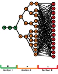
The results of the measurement and evaluation can be visualized as depicted in figure 1.
Fig. 1.The graphical representation the SCA result
We will call this visualization the enumeration tree. It consists of three sec-tions. The first section consists of the subkey bits that we consider recovered. After the iterations of the template attack all options but one were discarded. Section II consists of the subkeys that we have partial information on, but not enough to reduce the number of likely subkeys to one. The last section consists of the subkeys that we have very little to no information on. It contains all possible subkeys per layer.
The idea is that each node ni,j in the representation is located in thei’th level (starting with 1 at the root) and corresponds to the j’th choice for subkeys
ki,1, ki,2. . . ,. For each nodeni,j there is an associated subkey ki,j and a poste-rior probability qi,j. This is the probability that subkey iis equal toki,j given that the path up to its parent node is correct. So if the nodes on the path to
ni,j aren1,x1, n2,x2, . . . , ni−1,xi−1, ni,j, then the probabilityqi,j associated with this node is
qi,j= Pr[ki=ki,j|k1=k1,x1, k2=k2,x2, . . . , ki−1=ki−1,xi−1]. (1)
nodes leading up to it (including itself). This probability is then
pi,j=qi,j· i−1
Y
h=1
q1,xh. (2)
In sections I and II the subkeys that were discarded during the attack and are not in the model might have a combined small probability p. We assume that these probabilities are negligible (otherwise more nodes should be included in section II or the transition between section I and II should have moved closer to the root) and thus assume that the sum of the probabilitiespi,j of each level of the tree is 1.
3.2 Enumeration in an Interval
The brute-force approach an attacker could take to enumerate the keys is to sort the nodes of the rightmost layer of section II by posterior probability pij and then for each choice brute-force all the options in section III. However using the algorithms from Sections 2.3 and 2.4 we can do better. Enumerating section III of a node is equivalent to computing the keys in an interval. Therefore we can use the Pollard-kangaroo algorithms to speed up the enumeration. The downside of this approach is that without searching the whole interval we can never say with 100% certainty that the key is not in the interval. However, in return we are able to speed up enumeration in an interval of size ` to O(√`) group operations or even to O(√3
`) if we have the luxury of a precomputation table. We do have to note that even though we will call this process of searching the interval enumeration, it is a different kind than the enumeration in [17]. In that algorithm each key enumerated had to be checked for correctness against the encryption in an exhaustive-search manner. Using the kangaroo algorithms means that we search for a collision between group elements and only after this happens we can compute and double-check correctness against the public key of the cryptosystem attacked. This is much more sophisticated and much faster than the brute-force approach of having to check every key. The rankrofknow reflects the number of group operations required to find kafter the end of the experimental session. It also means that we have onlyO(√`) ranks and they are dependent on the parameters used in the algorithm. To accurately reflect the uncertainty in this kind of enumeration, we introduce the following definition.
Definition 1. Let the keyˆkthat we wish to find have rankrˆ. In an-enumeration
we check keys in such a way that when we have enumerated up to rank r, then there is a(1−)probability that ˆr > r.
Theorem 1. Assume that the private keykˆlies in the interval of size`. Let the average step size of the kangaroos be s =β√`. Let the probability of hitting a distinguished point be θ=c/√`and assume the distinguished points are spread uniformly over the whole group. Lastly we assume that the hash function H
and the step set in the improved Pollard-kangaroo algorithm of Section 2.3 is sufficiently random. Then forx > `/(4s)the average probability of not findingˆk
in2xsteps, i.e.xhops per kangaroo, of that algorithm is
(x) =e−xs+4`s2 + (eθ(4`s+2−x)−e2θ− 1 s(x−
`
4s))/(s−se(θ− 1
s)). (3)
Proof. Recall that in this algorithm we had 2 kangaroos placed in the interval and they alternate their jumps. In this proof we analyze thexsteps of the back kangaroo and compute the average probability that it does not collide with the front kangaroo even though they were both placed in the same interval. First the back kangaroo needs to catch up to the front one. The number of steps to do this is on average `/4s. Given that the back kangaroo takes xsteps we now have y=x−`/(4s) steps left on average. To avoid a recorded collision in these remainingysteps we either have to avoid the trail of the front kangaroo, or hit it afteristeps and avoid distinguished points for the nexty−isteps. We assumed the hash function H to be sufficiently random, so the average probability of avoiding the trail is (1−1/s) for each step taken and the chance of missing a distinguished point is (1−θ) in each step. Thus we have the average approximate probability of avoiding detected collisions as follows
1−1
s
x−4`s
+ x−`
4s−1
X
i=0
1−1
s
i
1
s(1−θ)
x−` 4s−i−2.
We can approximate the second part of this equation as follows
x−` 4s−1
X
i=0
1−1
s
i1
s(1−θ)
x−`
4s−i−2≈1
s
x−` 4s−1
X
i=0
e−is e−θ(x− `
4s−i−2) = e θ(`
4s+2−x)
s
x−` 4s−1
X
i=0
e−is eθi.
This in turn then evaluates to
eθ(4`s+2−x)
s
x−` 4s−1
X
i=0
eθ−1s
i
=e θ(`
4s+2−x)
s ·
1−e(θ−1s)(x− ` 4s)
1−e(θ−1s)
=e θ(`
4s+2−x)−e2θ− 1 s(x−
` 4s)
s−se(θ−1s)
.
So indeed we have our average probability of
(x) =
1−1
s
x−4`s +e
θ(`
4s+2−x)−e2θ− 1 s(x−
` 4s)
s−se(θ−1s)
≈e−xs+ ` 4s2+e
θ(`
4s+2−x)−e2θ− 1 s(x−
` 4s)
s−se(θ−1s)
.
Note that this equation is only valid for values ofx > 4`s, otherwise(x) = 1. We now analyze the situation of using Pollard’s kangaroo algorithm with a precomputation table. For this we make a hypothesis on the distribution of distinguished points and the number of points covered by each walk: Let the precomputation tableT consist of the first foundT different distinguished points
Di=tiP. Let the average walk length bew=α
p
`/T and the average step size of the kangaroos be s ≈ `/(4w) such that the average distance of a walk is
≈`/4. Since the points in T are different their paths are disjoint. They cover on average T wpoints. Assume that these points are uniformly distributed over
{P,2P, . . . , γ`P} for some value of γ. In Section 4 we will present experiments showing thatγ= max
1≤i≤Tti/`−1≤mini≤Tti/`is a good fit.
Theorem 2. Let ˆk lie in an interval of size `. Let the average walk length be
w =αp`/T and the average step size of the kangaroos be s ≈`/(4w). Under the hypothesis made above, T represents tW points distributed uniformly over
{P,2P, . . . , γ`P} for some value ofγ. The average probability that the Pollard-kangaroo algorithm with precomputation (Section 2.4) does not findˆkiny inde-pendent walks of the algorithm is
(x) =e−α
2y
γ . (4)
Proof. Under the hypothesis the probability of the wild kangaroo hitting the trail of one of the table points’ kangaroos is on average (T w)/(γ`) =α2/(γw) at each step. Since the walk takes on averagewsteps the probability of avoiding a collision is
1−α2/(γw)w
≈e−α
2 γ .
We assume independent walks, so we have that the probability that aftery
walks we have not found a collision is
y
Y
i=1
e−α
2 γ =e
−α2y γ .
which is the result we desired. ut
3.3 Further Considerations and Optimizations
separately is not searched because it is not part of some large combined inter-val. We therefore only combine intervals if they also have subsequent posterior probabilities. For the precomputation case of the algorithm we also have to take the availability of tables into account. We only combine intervals if we have a table and step set corresponding to that newly created interval length.
Restarts We described the general kangaroo algorithm to have the kangaroos continue along their paths after finding a distinguished point. For the standard rho method [2] show the benefits of restarting walks after a distinguished point is found. If we do not use a precomputation table then doing restarts means redoing the initial phase of the two kangaroos catching up to each other and the error function will decrease at a slower rate. This is only advantageous if the kangaroos ended up in a loop they cannot get out. If we detect such a loop, the kangaroo(s) can be restarted. If`n the probability of ending in a loop is very small. On the other hand, we do not have the problem of the initial catching up phase. Therefore we restarted walks if they exceeded 20wsteps. An advantage of using the improved Pollard-kangaroo algorithm without precomputation tables is that there is a probability of finding the solution of a DLP in an adjacent interval because the kangaroos naturally venture out in the direction of larger discrete logarithms. This is also an argument against doing restarts. Even though the current interval was chosen for the good reason of having the highest posterior probability among those not considered, yet, it is an added benefit that one might accidentally find a solution in another interval. If the tame kangaroo is started in intervalI1of size`, but the key was actually in adjacent intervalI2, then after a longer initial catch-up phase there is a probability of collisions. We could estimate this probability with an error function like we did forI1to reduce search time, but the longer the kangaroos jump the bigger the variance gets and the less accurate the error function is going to be. Therefore we do not advise to include this extra probability into the considerations.
Parallelization There are two levels at which the-enumeration method can be parallelized: One level is the underlying kangaroo algorithm using distinguished points; the second level is dividing the intervals over the processors used, i.e., we could simply place one interval search on each processor, or we could have all processors search one of the intervals, or use a combination of the two. Us-ing multiple processors for a sUs-ingle interval only makes sense if the interval is sufficiently large and many walks are needed (so rarely with precomputation) and if the posterior probability is significantly higher. If a lot of intervals have a similar probability it might be better to search them in parallel.
subkey in the enumeration tree with their probabilities. They are however not included in new templates, so the corresponding branch of the enumeration tree will not grow any more. After finishing the measurement we can determine with the error function for each interval with a higher posterior probability than the one that contains ˆkhow many steps we would (on average) take in this interval. The sum of these quantities is then an estimated lower bound for the rank of ˆk. We can use a similar method to determine an estimated upper bound.
4
Experimental Results
This section presents representative examples of our implementations. We ran our experiments on a Dell Optiplex 980 using one core of an Intel Core i5 Proces-sor 650 / 3.20GHz. We re-used parts of the Bernstein/Lange kangaroo C++ code used for [1]. Our adaptations will be posted athttp://www.scarecryptow.org/ publications/sckangaroos. For ease of implementation we used the groupF∗p as was used in [1], which uses a “strong” 256-bit prime (strong meaning that p−12 is also prime) and a generatorg, which is a large square modulop. Although in the previous sections we focussed on elliptic curves, both those andF∗pare cyclic groups and thus these results hold for both. We set the interval size to `= 248 and at each run took a randomhin the interval for a new DLP.
For the experiments without precomputation we made use of distinguished points to find the collision, which were recorded in a vector table that was searched each time a new distinguished point was found. We chose the probability of landing in a distinguished point to be 2−19 = √25
` by defining a point as distinguished if the least-significant 19 bits in its representation were zero, i.e., if the value modulo w= 219 was zero. The step function selected the next step based on the value modulo 128, the 128 step sizes were taken randomly around
√
`.
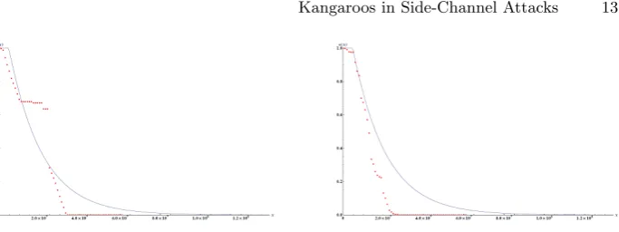
Step sets The goal of this paper is not to find the optimal parameters for the kangaroo algorithm. The choice of step set is however relevant for usability of the error function of Theorem 3. As can be seen equation 3 only uses the mean of the step set and not its actual values, so it is possible to create one that will not adhere to the error function at all. Even if we choose the step set randomly it can contain dependencies and this makes the error function less accurate. We can see this in the top graph of figure 2.
Fig. 2.The theoretic function(x) for the kangaroo method without precomputations and the experimental results using two random step setsS1 and S2 withβ≈1. Top: β= 0.978. Bottom:β= 0.971
set we found S2 which behaved nicely according to our expectations as can be observed in the bottom graph of figure 2. For concrete attacks it is advisable to run a few tests to check the quality of the step function.
Combining intervals We were able to find similar results for intervals where we combined two adjacent intervals of length 248to one of size 249. We observed the same problem of good and bad step sets. With trying three step sets, we got a step set that had the error function as an upper bound for the experiments. These graphs are similar to the graphs before and therefore ommitted. They did confirm that by combining the intervals we can search twice the keyspace in approximately √2 times the steps.
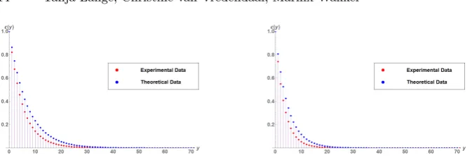
Using precomputation We again searched for DLPs in an interval of length 248. Our 128 step sizes however were now uniformly chosen between 0 and`/4w
instead of aroundβ√`for someβ. Each DLPh=gy was chosen randomly and each walk starting from it was randomized in the interval between y−240 and
y+ 240. For the precomputation we used a table of size N = T = √3
` = 216. We used the first T distinguished points found as table points and computed
γ= 1.923 as max
1≤i≤Tti/`−1≤mini≤Tti/`, for theT table elements of the formg ti. We
used an average walklength ofw= 215such thatα= 0.5. Using 2097152 experi-ments we got the results on the top of figure 3. We see that the error function is a good upper bound for the experimental results. We continued with the same ex-periment for an interval of length`= 250. We used a table ofT = 104032≈√3
`
table points and foundγ= 1.853. We used an average step set ofw= 216 such thatα≈0.630. Using 2097152 experiments we got the results on the bottom of figure 3. We again see that the error function is a good approximation for the experiments.
Fig. 3.The theoretic function(y) for the kangaroo method with precomputation and the experimental results using a step set withs≈ `
4w. Top:`= 2 48
. Bottom:`= 250.
mean, nor on how often distinguished points were found but it relies on the hypothesis that the table covers about wT points and these are uniformly dis-tributed over{P,2P, . . . , γP}.
Considerations about the step set are even more relevant when preparing the precomputation table by making N > T walks and selecting for T the T
points with the largest number of ancestors (longest walks leading up to them, distinguished points found with multiplicity).
For the-enumeration we suggest to include a parameterσin the exponent of the error function(y) =eσα2y/γthat is determined experimentally. After de-termining the step set and table we can run the algorithm on different randomly chosen DLPs, much like we did in our experiments, and determine a value for
σ. After this the error function is ready to be used in a security evaluation.
-Enumeration The result is that according to our best found results we can
-enumerate in an interval of length`in the steps displayed in table 1.
Table 1.Required group operations for-enumeration
1.0·10−1 1.0·10−31.0·10−5 1.0·10−71.0·10−9 N=T= 0, σ= 1 4.2·√` 10.8·√` 17.6·√` 24.3·√` 31.0·√` N=T=√3`, σ= 1 18·√3
` 54·√3
` 89·√3
` 124·√3
` 160·√3 ` N=T=√3`, σ= 1.12 16·√3
` 48·√3
` 79·√3
` 111·√3
` 142·√3 ` N= 2T = 2·√3
`, σ= 1 5·√3
` 14·√3
` 23·√3
` 32·√3
` 41·√3 ` N= 2T = 2·√3
`, σ= 1.28 4·√3
` 11·√3
` 18·√3
` 25·√3
` 32·√3 ` N= 8T = 8·√3
`, σ= 1 5·√3
` 14·√3
` 23·√3
` 31·√3
` 40·√3 ` N= 8T = 8·√3
`, σ= 1.40 4·√3
` 10·√3
` 16·√3
` 23·√3
` 29·√3 `
set. The results might thus be improved with optimal parameters. We observe that the higherN is relative to T, the fewer group operations are necessary to drop below the margin of error. Increasing the value ofNimproves the function-ality of the algorithm more than the variablesαandγreflect. This is seen in the experimental values ofσ. It increases asN increases. We also see that increasing
N from T to 2T makes a big difference in the required group operations. The effect of increasingN even further to 8T does not have the same magnitude.
Although even small speed-ups are always nice, we also have to take the time it takes to create the tables into account. ForN =T it took us just over 9 billion group operations and under 19 minutes to create the table. This is equal to 1.4√3
`2 multiplications. When we increased N to 2T it took about 50 minutes and 3.8√3
`2group operations. Finally, when we tookN up to 8T it took approximately 9 hours and 2.5 million walks of in total 161544244922≈37.6√3`2 group operations. This is doable for evaluation companies, even if they have to make a lot of tables, but doing many more might not have enough yield for the time it takes.
We see that we can determine how many group operations we have to do on average for different degrees of confidence. If we increase the confidence by a factor 100 the constantcinc√`orc√3
`increases linearly. This means that if we use theN = 8T precomputation table and we do 170√3`steps in an interval of length 248we can 2−128-enumerate it in less than 223.5group operations. This is a massive improvement over brute-force enumerating all 248keys in an interval. The new ranking method that is induced by such an enumeration is also a much more accurate measure of the security of a device. Security evaluation labs could more confidently estimate how secure an implementation is.
5
Comparison and Conclusion
This is the first paper studying key enumeration and rank estimates for public key cryptosystems. Gopalakrishnan, Th´eriault, and Yao [8] studied key recovery for ECC if a side-channel attack only provided some bits of the key. In contrast to our model they assume that the known bits are absolutely correct and do not discuss the possibility that we might have partial information on a subkey. If we were to make an enumeration tree of such a result it would solely consist of sections I and III. Although their assumption makes enumeration a lot easier it is not very realistic. Often there are too few bits fully recovered to make searching the remaining key space feasible. Using not only fully recovered bits but also the partial information we can search an interval smartly and possibly recover the solution to the DLP where [8] could not. Finally, they do not consider enumeration and rank computation.
5.1 Comparison
are adjacent and start from the most significant bits. This is true for the very common case of implementations using windowing methods (including signed and sliding) starting from the most significant bits. However, we can adjust our method to the scenarios considered in [8] as we will now discuss.
The first scenario in their paper is that contiguous bits of the key are re-vealed. These bits can be the most significant bits, the least significant bits or be somewhere in the middle. So far we considered the first case but our model can be easily adapted to the others:
– If the least significant bits are revealed, then our tree would get inverted. Searching section III would then require a slight adaptation of the algorithms used on it. Searching it with for instance Pollard kangaroo would require searching in equivalence classes instead of an interval. This adaptation means the probability of finding our solution ‘accidentally’ in a neighboring interval becomes zero. Creating tables in the Bernstein/Lange precomputation is still possible; we would shift each instance of the DLP to the same equivalence class.
– If bits somewhere in the middle are revealed the model would become more complicated. We would get a bow-shaped model with 2 sections II and III. There are 5 sections; the third contains known bits, on the second and fourth we have partial information and we have no information on the remaining sections. Enumerating through the sections III would become more compli-cated, though not impossible.
The second scenario [8] poses is that the information is not on any specific bits, but on the square-and-multiply chain. In this case the enumeration tree of figure 1 would become a binary tree. Searching the sections is the same as before.
an error function for these algorithms, but expect results similar to Theorems 1 and 2.
Lastly, it was pointed out to us by a kind anonymous reviewer that there are attacks on ECC where in fact the subkeys are independent (see e.g. [4,19,20]). In this case the rank estimation algorithm of [18] is applicable. The methods in this paper can then still be used as a comparison method; it is more realistic to compare dependent subkey attacks to independent ones with a-rank than the brute-force rank.
5.2 Conclusion
In summary, we showed that kangaroos can be very useful in making SCA on ECC more efficient:
– Once section III is below 80 bits and section II not too wide there is no point in letting the lab guy do further measurements since a standard PC can casually do the 240 group operations to break the DLP.
– In cases where measurements cannot be pushed further by physical limita-tions (restricted number of measurements, limits on what templates can be measured) our improvements allow retrieving the key in some situations in which previous methods could not.
– Theoretical kangaroos can be used to estimate the rank of the key in white-box scenarios to determine whether a sufficiently motivated attacker could mount the attack to break the system and we present error functions to use in-enumeration.
References
1. Daniel J. Bernstein and Tanja Lange. Computing small discrete logarithms faster. In Steven D. Galbraith and Mridul Nandi, editors,INDOCRYPT, volume 7668 of Lecture Notes in Computer Science, pages 317–338. Springer, 2012.
2. Daniel J. Bernstein, Tanja Lange, and Peter Schwabe. On the correct use of the negation map in the pollard rho method. In Dario Catalano, Nelly Fazio, Rosario Gennaro, and Antonio Nicolosi, editors,Public Key Cryptography, volume 6571 of Lecture Notes in Computer Science, pages 128–146. Springer, 2011.
3. Suresh Chari, Josyula R. Rao, and Pankaj Rohatgi. Template attacks. In Burton S. Kaliski Jr., C¸ etin Kaya Ko¸c, and Christof Paar, editors,CHES, volume 2523 of Lecture Notes in Computer Science, pages 13–28. Springer, 2002.
4. Christophe Clavier, Benoit Feix, Georges Gagnerot, Myl`ene Roussellet, and Vin-cent Verneuil. Horizontal correlation analysis on exponentiation. In Miguel So-riano, Sihan Qing, and Javier L´opez, editors, Information and Communications Security - 12th International Conference, ICICS 2010, Barcelona, Spain, Decem-ber 15-17, 2010. Proceedings, volume 6476 ofLecture Notes in Computer Science, pages 46–61. Springer, 2010.
6. Steven D. Galbraith and Raminder S. Ruprai. An improvement to the Gaudry-Schost algorithm for multidimensional discrete logarithm problems. In Matthew G. Parker, editor,IMA Int. Conf., volume 5921 ofLecture Notes in Computer Science, pages 368–382. Springer, 2009.
7. Pierrick Gaudry and ´Eric Schost. A low-memory parallel version of Matsuo, Chao, and Tsujii’s algorithm. In Duncan A. Buell, editor,ANTS, volume 3076 ofLecture Notes in Computer Science, pages 208–222. Springer, 2004.
8. K. Gopalakrishnan, Nicolas Th´eriault, and Chui Zhi Yao. Solving discrete log-arithms from partial knowledge of the key. In K. Srinathan, C. Pandu Rangan, and Moti Yung, editors,INDOCRYPT, volume 4859 ofLecture Notes in Computer Science, pages 224–237. Springer, 2007.
9. Darrel Hankerson, Alfred J. Menezes, and Scott Vanstone.Guide to Elliptic Curve Cryptography. Springer-Verlag New York, Inc., Secaucus, NJ, USA, 2003. 10. Jing Pan, Jasper G. J. van Woudenberg, Jerry den Hartog, and Marc F. Witteman.
Improving DPA by peak distribution analysis. In Alex Biryukov, Guang Gong, and Douglas R. Stinson, editors,Selected Areas in Cryptography, volume 6544 ofLecture Notes in Computer Science, pages 241–261. Springer, 2010.
11. John M. Pollard. Monte Carlo methods for index computation (mod p). Mathe-matics of Computation, 32:918–924, 1978.
12. John M. Pollard. Kangaroos, monopoly and discrete logarithms. J. Cryptology, 13(4):437–447, 2000.
13. Daniel Shanks. Class number, a theory of factorization, and genera. In Donald J. Lewis, editor,1969 Number Theory Institute, volume 20 ofProceedings of Symposia in Pure Mathematics, pages 415–440, Providence, Rhode Island, 1971. American Mathematical Society.
14. Andreas Stein and Edlyn Teske. The parallelized Pollard kangaroo method in real quadratic function fields. Math. Comput., 71(238):793–814, 2002.
15. Ernst G. Straus. Addition chains of vectors (problem 5125). American Mathe-matical Monthly, 70:806–808, 1964. URL: http://cr.yp.to/bib/entries.html# 1964/straus.
16. Paul C. van Oorschot and Michael J. Wiener. Parallel collision search with crypt-analytic applications. J. Cryptology, 12(1):1–28, 1999.
17. Nicolas Veyrat-Charvillon, Benoˆıt G´erard, Mathieu Renauld, and Fran¸cois-Xavier Standaert. An optimal key enumeration algorithm and its application to side-channel attacks. In Lars R. Knudsen and Huapeng Wu, editors,Selected Areas in Cryptography, volume 7707 ofLecture Notes in Computer Science, pages 390–406. Springer, 2012.
18. Nicolas Veyrat-Charvillon, Benoˆıt G´erard, and Fran¸cois-Xavier Standaert. Security evaluations beyond computing power. In Thomas Johansson and Phong Q. Nguyen, editors,EUROCRYPT, volume 7881 ofLecture Notes in Computer Science, pages 126–141. Springer, 2013.
19. Colin D. Walter. Sliding windows succumbs to big mac attack. In Proceedings of the Third International Workshop on Cryptographic Hardware and Embedded Systems, CHES ’01, pages 286–299, London, UK, UK, 2001. Springer-Verlag. 20. Marc F. Witteman, Jasper G. J. van Woudenberg, and Federico Menarini.