Recursive Principal Components Analysis Using Eigenvector Matrix Perturbation

(1)

Recursive Principal Components Analysis

Using Eigenvector Matrix Perturbation

Deniz Erdogmus

Department of Computer Science and Engineering, CSE, Oregon Graduate Institute, Oregon Health & Science University, Beaverton, OR 97006, USA

Email:[email protected]

Yadunandana N. Rao

Computational NeuroEngineering Laboratory (CNEL), Department of Electrical & Computer Engineering (ECE), University of Florida, Gainesville, FL 32611, USA

Hemanth Peddaneni

Anant Hegde

Jose C. Principe

Received 4 December 2003; Revised 19 March 2004; Recommended for Publication by John Sorensen

Principal components analysis is an important and well-studied subject in statistics and signal processing. The literature has an abundance of algorithms for solving this problem, where most of these algorithms could be grouped into one of the following three approaches: adaptation based on Hebbian updates and deflation, optimization of a second-order statistical criterion (like reconstruction error or output variance), and fixed point update rules with deflation. In this paper, we take a completely diﬀ er-ent approach that avoids deflation and the optimization of a cost function using gradier-ents. The proposed method updates the eigenvector and eigenvalue matrices simultaneously with every new sample such that the estimates approximately track their true values as would be calculated from the current sample estimate of the data covariance matrix. The performance of this algorithm is compared with that of traditional methods like Sanger’s rule and APEX, as well as a structurally similar matrix perturbation-based method.

Keywords and phrases:PCA, recursive algorithm, rank-one matrix update.

1. INTRODUCTION

Principal components analysis (PCA) is a well-known statis-tical technique that has been widely applied to solve impor-tant signal processing problems like feature extraction,

sig-nal estimation, detection, and speech separation [1,2,3,4].

Many analytical techniques exist, which can solve PCA once

the entire input data is known [5]. However, most of the

analytical methods require extensive matrix operations and

hence they are unsuited for real-time applications. Further, in many applications such as direction of arrival (DOA) tracking, adaptive subspace estimation, and so forth, signal statistics change over time rendering the block methods vir-tually unacceptable. In such cases, fast, adaptive, on-line so-lutions are desirable. Majority of the existing algorithms for

PCA are based on standard gradient procedures [2,3,6,7,

8,9], which are extremely slow converging, and their

(2)

subspace methods have been explored [10, 11, 12]. How-ever, many of these subspace techniques are computation-ally intensive. The recently proposed fixed-point PCA

algo-rithm [13] showed fast convergence with little or no change

in complexity compared with gradient methods. However, this method and most of the existing methods in literature rely on using the standard deflation technique, which brings in sequential convergence of principal components that po-tentially reduces the overall speed of convergence. We re-cently explored a simultaneous principal component

extrac-tion algorithm called SIPEX [14] which reduced the gradient

search only to the space of orthonormal matrices by using Givens rotations. Although SIPEX resulted in fast and simul-taneous convergence of all principal components, the

algo-rithm suﬀered from high computational complexity due to

the involved trigonometric function evaluations. A recently proposed alternative approach suggested iterating the eigen-vector estimates using a first-order matrix perturbation for-malism for the sample covariance estimate with every new

sample obtained in real time [15]. However, the performance

(speed and accuracy) of this algorithm is hindered by the general Toeplitz structure of the perturbed covariance ma-trix. In this paper, we will present an algorithm that under-takes a similar perturbation approach, but in contrast, the covariance matrix will be decomposed into its eigenvectors and eigenvalues at all times, which will reduce the pertur-bation step to be employed on the diagonal eigenvalue ma-trix. This further restriction of structure, as expected,

allevi-ates the diﬃculties encountered in the operation of the

pre-vious first-order perturbation algorithm, resulting in a fast converging and accurate subspace tracking algorithm.

This paper is organized as follows. First, we present a brief definition of the PCA problem to have a self-contained paper. Second, the proposed recursive PCA (RPCA) algo-rithm is motivated, derived, and extended to non-stationary and complex-valued signal situations. Next, a set of com-puter experiments is presented to demonstrate the conver-gence speed and accuracy characteristics of RPCA. Finally, we conclude the paper with remarks and observations about the algorithm.

2. PROBLEM DEFINITION

PCA is a well-known problem and is extensively studied in the literature as we have pointed out in the introduction. However, for the sake of completeness, we will provide a brief definition of the problem in this section. For simplicity, and without loss of generality, we will consider a real-valued

zero-mean,n-dimensional random vectorxand itsnprojections

y1,. . .,y_nsuch thaty_j=wT_jx, wherew_j’s are unit-norm

vec-tors defining the projection dimensions in then-dimensional

input space.

The first principal component direction is defined as the solution to the following constrained optimization problem,

whereRis the input covariance matrix:

w1=arg max

w

wTRw subject towTw=1. (1)

The subsequent principal components are defined by includ-ing additional constraints to the problem that enforce the or-thogonality of the sought component to the previously dis-covered ones:

wj=arg max

w w

T_Rw_, _s.t._wT_w₌_1,_wT_w_l₌_0, _{l < j.} ₍₂₎

The overall solution to this problem turns out to be

the eigenvector matrix of the input covariance R. In

par-ticular, the principal component directions are given by the

eigenvectors ofRarranged according to their corresponding

eigenvalues (largest to smallest) [5].

In signal processing applications, the needs are diﬀ

er-ent. The input samples are usually acquired one at a time (i.e., sequentially as opposed to in batches), which necessi-tates sample-by-sample update rules for the covariance and its eigenvector estimates. In this setting, this analytical solu-tion is of little use, since it is not practical to update the in-put covariance estimate and solve a full eigendecomposition problem per sample. However, utilizing the recursive struc-ture of the covariance estimate, it is possible to come up with a recursive formula for the eigenvectors of the covariance as well. This will be described in the next section.

3. RECURSIVE PCA DESCRIPTION

Suppose a sequence ofn-dimensional zero-mean wide-sense

stationary input vectorsx_kare arriving, wherekis the sample

(time) index. The sample covariance estimate at timekfor

the input vector is1

R_k=1

Λ denote the orthonormal eigenvector and diagonal

eigen-value matrices, respectively. Also defineαk=QT_k₋₁xk.

Substi-tuting these definitions in (3), we obtain the following

recur-sive formula for the eigenvectors and eigenvalues:

QkkΛkQT_k =Qk−1

(k−1)Λk−1+αkαT_k

QT_k₋₁. (4)

Clearly, if we can determine the eigendecomposition of the

matrix [(k−1)Λ_k−1+αkαT_k], which is denoted byVkDkVT_k,

whereVis orthonormal andDis diagonal, then (4) becomes

Q_kkΛ_kQT_k =Q_k−1VkDkVT_kQT_k−1. (5)

1_{In practice, if the samples are not generated by a zero-mean process, a}

(3)

By direct comparison, the recursive update rules for the eigenvectors and the eigenvalues are determined to be

Qk=Qk−1Vk,

Λk=D_{k .}k

(6)

In spite of the fact that the matrix [(k−1)Λk−1+αkαT_k] has a

special structure much simpler than that of a general

covari-ance matrix, determining the eigendecompositionV_kD_kVT_k

analytically is diﬃcult. However, especially ifkis large, the

problem can be solved in a simpler way using a matrix per-turbation analysis approach. This will be described next.

3.1. Perturbation analysis for rank-one update

Whenkis large, the matrix [(k−1)Λk−1+αkαT_k] is strongly

diagonally dominant; hence (due to the Gershgorin theorem) its eigenvalues will be close to those of the diagonal portion

(k−1)Λ_k−1. In addition, its eigenvectors will also be close to

identity (i.e., the eigenvectors of the diagonal portion of the sum).

In summary, the problem reduces to finding the

eigen-decomposition of a matrix in the form (Λ+ααT), that is, a

rank-one update on a diagonal matrixΛ, using the following

approximations:D=Λ+P_ΛandV=I+PV, wherePΛand

PVare small perturbation matrices. The eigenvalue

perturba-tion matrixPΛis naturally diagonal. With these definitions,

whenVDVTis expanded, we get

VDVT =I+PV

The orthonormality ofVbrings an additional equation that

characterizesPV. SubstitutingV=I+PVinVVT =I, and

assuming thatPVPTV≈0, we havePV= −PTV.

Combining the fact that the eigenvector perturbation

matrix PV is antisymmetric with the fact that PΛ and D

are diagonal, the solutions for the perturbation matrices are

found from (8) as follows: theith diagonal entry ofPΛisα2_i

and the (i,j)th entry ofPVisαiαj/(λj+α2j−λi−α2i) ifj=i,

and 0 if j=i.

3.2. The recursive PCA algorithm

The RPCA algorithm is summarized inAlgorithm 1. There

are a few practical issues regarding the operation of the algo-rithm, which will be addressed in this subsection.

(1) InitializeQ0andΛ0.

(2) At each time instantkdo the following. (a) Get input samplexk.

(b) Set memory depth parameterλk. (c) Calculateαk=QTk−1xk.

(d) Find perturbationsPVandPΛcorresponding to

1−λkΛk−1+λkαkαTk.

(e) Update eigenvector and eigenvalue matrices:

(f) Normalize the norms of eigenvector estimates byQk=QkTk, whereTkis a diagonal matrix containing the inverses of the norms of each column ofQk.

(g) Correct eigenvalue estimates byΛk=ΛkT−k2, whereT−2

k is a diagonal matrix containing the squared norms of the columns ofQk.

Algorithm1: The recursive PCA algorithm outline.

Selecting the memory depth parameter

In a stationary situation, where we would like to weight each individual sample equally, this parameter must be set to

λk=1/k. In this case, the recursive update for the covariance

matrix is as shown in (3). In a nonstationary environment, a

first-order dynamical forgetting strategy could be employed

by selecting a fixed decay rate. Settingλk=λcorresponds to

the following recursive covariance update equation:

Rk=(1−λ)Rk+λxkxT_k. (9)

Typically, in this forgetting scheme,λ ∈(0, 1) is selected to

be very small. Considering that the average memory depth of

this recursion is 1/λsamples, the selection of this parameter

presents a trade-oﬀbetween tracking capability and

estima-tion variance.

Initializing the eigenvectors and the eigenvalues

The natural way to initialize the eigenvector matrixQ0and

the eigenvalue matrixΛ0is to use the firstN0samples to

ob-tain an unbiased estimate of the covariance matrix and

de-termine its eigendecomposition (N0 > n). The iterations in

step (2) can then be applied to the following samples. This

means in step (2)k =N0+ 1,. . .,N. In the stationary case

(λk =1/k), this means in the first few iterations of step (2)

the perturbation approximations will be least accurate (com-pared to the subsequent iterations). This is simply due to

(1−λk)Λk−1+λkαkαT_k not being strongly diagonally

dom-inant for small values ofk. Compensating the errors induced

in the estimations at this stage might require a large number of samples later on.

This problem could be avoided if in the iteration stage

(step (2)) the index k could be started from a large initial

(4)

to the estimates, one needs to use a large number of

sam-ples in the initialization (i.e., choose a large N0). In

prac-tice, however, this is undesirable. The alternative is to per-form the initialization still using a small number of samples

(i.e., a smallN0), but setting the memory depth parameter to

λk = 1/(k+ (τ−1)N0). This way, when the iterations start

at samplek=N0+ 1, the algorithmthinksthat the

initializa-tion is actually performed usingγ=τN0samples. Therefore,

from the point of view of the algorithm, the data set looks like

The corresponding covariance estimator is then naturally bi-ased. At the end of the iterations, the estimated covariance matrix is

that the bias introduced to the estimation by tricking the

al-gorithm can be asymptotically diminished (asN→ ∞).

In practice, we actually do not want to solve for an eigen-decomposition problem at all. Therefore, one could simply

initialize the estimated eigenvector to identity (Q0 =I) and

the eigenvalues to the sample variances of each input entry

overN0samples (Λ0=diagRN0). We then start the iterations

over the samplesk=1,. . .,Nand set the memory depth

pa-rameter toλk=1/(k−1 +γ). Eﬀectively this corresponds to

the following biased (but asymptotically unbiased asN→ ∞)

covariance estimate:

R_N,biased=_NN

+γRN+

γ

N+γΛ0. (12)

This latter initialization strategy is utilized in all the com-puter experiments that are presented in the following

sec-tions.2

In the case of a forgetting covariance estimator (i.e.,λk=

λ), the initialization bias is not a problem, since its eﬀect

will diminish in accordance with the forgetting time constant any way. Therefore, in the nonstationary case, once again, we

suggest using the latter initialization strategy: Q0 = I and

Λ0 =diagRN0. In this case, in order to guarantee the

accu-racy of the first order perturbation approximation, we need

to choose the forgetting factorλsuch that the ratio (1−λ)/λ

is large. Typically, a forgetting factorλ < 10−2_{will yield}

ac-curate results, although if necessary values up toλ = 10−1

could be utilized.

2_{A further modification that might be installed is to use a time-varying}

γvalue. In the experiments, we used an exponentially decaying profile for γ,γ=γ0exp(−k/τ). This forces the covariance estimation bias to diminish

even faster.

3.3. Extension to complex-valued PCA

The extension of RPCA to complex-valued signals is triv-ial. Basically, all matrix-transpose operations need to be re-placed by Hermitian (conjugate-transpose) operators. Be-low, we briefly discuss the derivation of the complex-valued RPCA algorithm following the steps of the real-valued ver-sion.

The sample covariance estimate for zero-mean complex data is given by

Rk=1_k

the eigenvalues are still real-valued in this case, but the

eigen-vectors are complex eigen-vectors. Definingα_k =QH_k₋₁x_k and

fol-lowing the same steps as in (4) to (8), we determine that

PV = −PHV. Therefore, as opposed to the expressions

de-rived in Section 3.1, here the complex conjugation ∗ and

magnitude| · |operations are utilized. Theith diagonal

en-try ofP_Λis found to be|αi|2and the (i,j)th entry ofPVis

αiα∗j/(λj+|αj|2−λi− |αi|2) ifj=i, and 0 ifj=i. The

algo-rithm inAlgorithm 1is utilized as it is except for the

modifi-cations mentioned in this section.

4. NUMERICAL EXPERIMENTS

The PCA problem is extensively studied in the literature and there exist an excessive variety of algorithms to solve this problem. Therefore, an exhaustive comparison of the pro-posed method with existing algorithms is not practical. In-stead, a comparison with a structurally similar algorithm (which is also based on first-order matrix perturbations)

will be presented [15]. We will also comment on the

per-formances of traditional benchmark algorithms like Sanger’s rule and APEX in similar setups, although no explicit de-tailed numerical results will be provided.

4.1. Convergence speed analysis

In the first experimental setup, the goal is to investigate the convergence speed and accuracy of the RPCA algorithm. For

this, n-dimensional random vectors are drawn from a

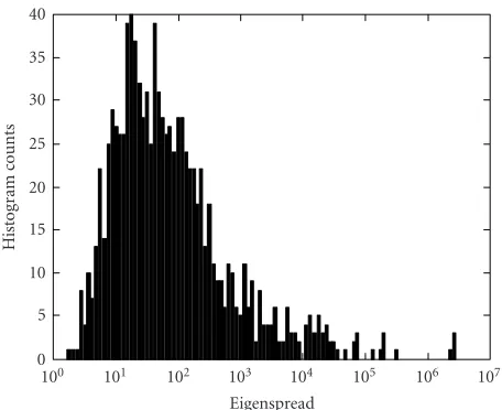
nor-mal distribution with an arbitrary covariance matrix. In par-ticular, the theoretical covariance matrix of the data is given

byAAT, whereAis ann×nreal-valued matrix whose

en-tries are drawn from a zero-mean unit-variance Gaussian distribution. This process results in a wide range of

eigen-spreads (as shown inFigure 1), therefore the convergence

re-sults shown here encompass such eﬀects.

Specifically, the results of the 3-dimensional case study are presented here, where the data is generated by 3-dimensional normal distributions with randomly selected covariance matrices. A total of 1000 simulations (Monte Carlo runs) are carried out for each of the three target eigen-vector estimation accuracies (measured in terms of degrees

between the estimated and actual eigenvectors): 10◦, 5◦, and

(5)

100 ₁₀1 ₁₀2 ₁₀3 ₁₀4 ₁₀5 ₁₀6 ₁₀7

Figure1: Distribution of eigenspread values forAAT, whereA3×3

is generated to have Gaussian distributed random entries.

of iterations it takes the algorithm to converge to the target eigenvector accuracy in all eigenvectors (not just the princi-pal component). The histograms of convergence times (up to 10000 samples) for these three target accuracies are shown in

Figure 2, where everything above 10000 is also lumped into the last bin. In these Monte Carlo runs, the initial eigenvector estimates were set to the identity matrix and the randomly selected data covariance matrices were forced to have eigen-vectors such that all the initial eigenvector estimation errors

were at least 25◦. The initialγvalue was set to 400 and the

decay time constant was selected to be 50 samples. Values in this range were found to work best in terms of final accuracy and convergence speed in extensive Monte Carlo runs.

It is expected that there are some cases, especially those with high eigenspreads, which require a very large number of samples to achieve very accurate eigenvector estimations, especially for the minor components. The number of iter-ations required for convergence to a certain accuracy level is also expected to increase with the dimensionality of the prob-lem. For example, in the 3-dimensional case, about 2% of the

simulations failed to converge within 10◦in 10000 on-line

it-erations, whereas this ratio is about 17% for 5 dimensions. The failure to converge within the given number of iterations

is observed for eigenspreads over 5×104_.

In a similar setup, Sanger’s rule achieves a mean conver-gence speed of 8400 iterations with a standard deviation of 2600 iterations. This results in an average eigenvector

direc-tion error of about 9◦with a standard deviation of 8◦. APEX

on the other hand converges rarely to within 10◦. Its

aver-age eigenvector direction error is about 30◦with a standard

deviation of 15◦.

4.2. Comparison with first-order perturbation PCA

The first-order perturbation PCA algorithm [15] is

struc-turally similar to the RPCA algorithm presented here. The

main diﬀerence is the nature of the perturbed matrix: the

former works on a perturbation approximation for the

com-plete covariance matrix, whereas the latter considers the per-turbation of a diagonal matrix. We expect this structural re-striction to improve performance in terms of overall algo-rithm performance. To test this hypothesis, an experimental

setup similar to the one inSection 4.1is utilized. This time,

however, the data is generated by a colored time series us-ing a time-delay line (makus-ing the procedure a temporal PCA case study). Gaussian white noise is colored using a two-pole filter whose poles are selected from a random uniform distri-bution on the interval (0, 1). A set of 15 Monte Carlo simula-tions was run on 3-dimensional data generated according to this procedure. The two parameters of the first-order

pertur-bation method were set toε=10−3_/₆_._{5 and}_δ ₌₁₀−2_{. The}

parameters of RPCA were set toγ0 =300 andτ =100. The

average eigenvector direction estimation convergence curves

are shown inFigure 3.

Often, signal subspace tracking is necessary in signal pro-cessing applications dealing with nonstationary signals. To illustrate the performance of RPCA for such cases, a piece-wise stationary colored noise sequence is generated by filter-ing white Gaussian noise with sfilter-ingle-pole filters with the fol-lowing poles: 0.5, 0.7, 0.3, 0.9 (in order of appearance). The

forgetting factor is set to a constantλ =10−3_{. The two}

pa-rameters of the first-order perturbation method were again

set toε =10−3_/₆_._{5 and}_δ ₌ ₁₀−2_{. The results of 30 Monte}

Carlo runs were averaged to obtainFigure 4.

4.3. Direction of arrival estimation

The use of subspace methods for DOA estimation in sensor

arrays has been extensively studied (see [14] and the

refer-ences therein). In Figure 5, a sample run from a computer

simulation of DOA according to the experimental setup

de-scribed in [14] is presented to illustrate the performance of

the complex-valued RPCA algorithm. To provide a bench-mark (and an upper limit in convergence speed), we also

performed this simulation using Matlab’seigfunction several

times on the sample covariance estimate. The latter typically converged to the final accuracy demonstrated here within 10–20 samples. The RPCA estimates on the other hand take

a few hundred samples due to the transient in theγ value.

The main diﬀerence in the application of RPCA is that typical

DOA algorithm will convert the complex PCA problem into a structured PCA problem with double the number of dimen-sions, whereas the RPCA algorithm works directly with the complex-valued input vectors to solve the original complex PCA problem.

4.4. An example with 20 dimensions

(6)

0 5000 10000

Figure2: The convergence time histograms for RPCA in the 3-dimensional case for three diﬀerent target accuracy levels: (a) target error =10◦, (b) target error=5◦, and (c) target error=2◦.

0 1000 2000 3000 4000 5000 6000 7000 8000 9000 10000 Iterations

Figure3: The average eigenvector direction estimation errors, de-fined as the angle between the actual and the estimated eigenvectors, versus iterations are shown for the first-order perturbation method (thin dotted lines) and for RPCA (thick solid lines).

competing structural properties of the eigenspace makes a

compromise from one or the other increasingly diﬃcult.

Specifically, these two characteristics are the eigenspread

(maxλi/minλi) and the distribution of ratios of consecutive

eigenvalues (λ_n/λ_n−1,. . .,λ2/λ1) when they are ordered from

Figure4: The average eigenvector direction estimation errors, de-fined as the angle between the actual and the estimated eigenvectors, versus iterations for the first-order perturbation method (thin dot-ted lines) and for RPCA (thick solid lines) in a piecewise station-ary situation are shown. The eigenstructure of the input abruptly changes every 5000 samples.

(7)

100 ₁₀1 ₁₀2 ₁₀3

Figure5: Direction of arrival estimation in a linear sensor array using complex-valued RPCA in a 3-source 6-sensor case.

to the same reason, smaller and previously acceptable eigen-spread values too become undesirable because consecutive eigenvalues approach each other. This causes the discrim-inability of the eigenvectors corresponding to these eigen-values diminish as their ratio approaches unity. Therefore,

the trade-oﬀbetween small and large eigenspreads becomes

significantly diﬃcult. Ideally, the ratios between consecutive

eigenvalues must be identical for equal discriminability of all subspace components. Variations from this uniformity will result in faster convergence in some eigenvectors, while

oth-ers will suﬀer from almost spherical subspaces

indiscrim-inability.

InFigure 6, the convergence of the 20 estimated eigenvec-tors to their corresponding true values is illustrated in terms of the angle between them (in degrees) versus the number of on-line iterations. The data is generated by a 20-dimensional jointly Gaussian distribution with zero mean, and a covari-ance matrix with eigenvalues equal to the powers (from 0

to 19) of 1.5 and eigenvectors selected randomly.3 _This

re-sult is typical of higher-dimensional cases where major com-ponents converge relatively fast and minor comcom-ponents take much longer (in terms of samples and iterations) to reach the same level of accuracy.

5. CONCLUSIONS

In this paper, a novel approximate fixed-point algorithm for subspace tracking is presented. The fast tracking capability is enabled by the recursive nature of the complete eigenvec-tor matrix updates. The proposed algorithm is feasible for real-time implementation since the recursions are based on well-structured matrix multiplications that are the conse-quences of the rank-one perturbation updates exploited in

3_{This corresponds to an eigenspread of 1}_.₅19_≈_2217.

0 0_.5 1 1_.5 2 2_.5 3 3_.5 4 4_.5 5

Figure6: The convergence of the angle error between the estimated eigenvectors (using RPCA) and their corresponding true eigenvec-tors in a 20-dimensional PCA problem is shown versus on-line iter-ations.

the derivation of the algorithm. Performance comparisons with traditional algorithms as well as a structurally simi-lar perturbation-based approach demonstrated the advan-tages of the recursive PCA algorithm in terms of convergence speed and accuracy.

ACKNOWLEDGMENT

This work is supported by NSF Grant ECS-0300340.

REFERENCES

[1] R. O. Duda and P. E. Hart, Pattern Classification and Scene Analysis, John Wiley & Sons, New York, NY, USA, 1973. [2] S. Y. Kung, K. I. Diamantaras, and J. S. Taur, “Adaptive

prin-cipal component extraction (APEX) and applications,” IEEE Trans. Signal Processing, vol. 42, no. 5, pp. 1202–1217, 1994. [3] J. Mao and A. K. Jain, “Artificial neural networks for feature

extraction and multivariate data projection,” IEEE Transac-tions on Neural Networks, vol. 6, no. 2, pp. 296–317, 1995. [4] Y. Cao, S. Sridharan, and A. Moody, “Multichannel speech

separation by eigendecomposition and its application to co-talker interference removal,” IEEE Trans. Speech and Audio Processing, vol. 5, no. 3, pp. 209–219, 1997.

[5] G. H. Golub and C. F. Van Loan,Matrix Computations, Johns Hopkins University Press, Baltimore, Md, USA, 1983. [6] E. Oja, Subspace Methods for Pattern Recognition, John Wiley

& Sons, New York, NY, USA, 1983.

[7] T. D. Sanger, “Optimal unsupervised learning in a single-layer linear feedforward neural network,” Neural Networks, vol. 2, no. 6, pp. 459–473, 1989.

[8] J. Rubner and K. Schulten, “Development of feature detectors by self-organization: a network model,”Biological Cybernetics, vol. 62, no. 3, pp. 193–199, 1990.

[9] J. Rubner and P. Tavan, “A self-organizing network for principal-component analysis,” Europhysics Letters, vol. 10, no. 7, pp. 693–698, 1989.

(8)

[11] B. Yang, “Projection approximation subspace tracking,”IEEE Trans. Signal Processing, vol. 43, no. 1, pp. 95–107, 1995. [12] Y. Hua, Y. Xiang, T. Chen, K. Abed-Meraim, and Y. Miao,

“Natural power method for fast subspace tracking,” inProc. IEEE Neural Networks for Signal Processing, pp. 176–185, Madison, Wis, USA, August 1999.

[13] Y. N. Rao and J. C. Principe, “Robust on-line principal component analysis based on a fixed-point approach,” in Proc. IEEE Int. Conf. Acoustics, Speech, Signal Processing, vol. 1, pp. 981–984, Orlando, Fla, USA, May 2002.

[14] D. Erdogmus, Y. N. Rao, K. E. Hild II, and J. C. Principe, “Si-multaneous principal-component extraction with application to adaptive blind multiuser detection,”EURASIP. J. Appl. Sig-nal Process., vol. 2002, no. 12, pp. 1473–1484, 2002.

[15] B. Champagne, “Adaptive eigendecomposition of data co-variance matrices based on first-order perturbations,” IEEE Trans. Signal Processing, vol. 42, no. 10, pp. 2758–2770, 1994.

Deniz Erdogmusreceived his B.S. degrees in electrical engineering and mathematics in 1997, and his M.S. degree in electrical engineering, with emphasis on systems and control, in 1999, all from the Middle East Technical University, Turkey. He received his Ph.D. in electrical engineering from the University of Florida, Gainesville, in 2002. Since 1999, he has been with the Computa-tional NeuroEngineering Laboratory,

Uni-versity of Florida, working with Jose Principe. His current research interests include information-theoretic aspects of adaptive signal processing and machine learning, as well as their applications to problems in communications, biomedical signal processing, and controls. He is the recipient of the IEEE SPS 2003 Young Author Award, and is a Member of IEEE, Tau Beta Pi, and Eta Kappa Nu.

Yadunandana N. Raoreceived his B.E. de-gree in electronics and communication en-gineering in 1997, from the University of Mysore, India, and his M.S. degree in elec-trical and computer engineering in 2000, from the University of Florida, Gainesville, Fla. From 2000 to 2001, he worked as a de-sign engineer at GE Medical Systems, Wis. Since 2001, he has been working toward his Ph.D. in the Computational

NeuroEngi-neering Laboratory (CNEL) at the University of Florida, under the supervision of Jose C. Principe. His current research interests in-clude design of neural analog systems, principal components anal-ysis, generalized SVD with applications to adaptive systems for sig-nal processing and communications.

Hemanth Peddanenireceived his B.E. de-gree in electronics and communication en-gineering from Sri Venkateswara University, Tirupati, India, in 2002. He is now pursu-ing his Master’s degree in electrical engi-neering at the University of Florida. His re-search interests include neural networks for signal processing, adaptive signal process-ing, wavelet methods for time series anal-ysis, digital filter design/implementation, and digital image processing.

Anant Hegdegraduated with an M.S. de-gree in electrical engineering from the Uni-versity of Houston, Tex. During his Mas-ter’s, he worked in the Bio-Signal Anal-ysis Laboratory (BSAL) with his research mainly focusing on understanding the pro-duction mechanisms of event-related po-tentials such as P50, N100, and P300. Hegde is currently pursuing his Ph.D. research in the Computational NeuroEngineering

Lab-oratory (CNEL) at the University of Florida, Gainesville. His focus is on developing signal processing techniques for detecting asym-metric dependencies in multivariate time structures. His research interests are in EEG analysis, neural networks, and communication systems.

Jose C. Principeis a Distinguished Profes-sor of Electrical and Computer Engineering and Biomedical Engineering at the Univer-sity of Florida, where he teaches advanced signal processing, machine learning, and ar-tificial neural networks (ANNs) modeling. He is BellSouth Professor and the Founder and Director of the University of Florida Computational NeuroEngineering Labora-tory (CNEL). His primary area of interest