R E S E A R C H
Open Access
Initial condition for efficient mapping of level
set algorithms on many-core architectures
Gábor János Tornai
*and György Cserey
Abstract
In this paper, we investigated the effect of adding more small curves to the initial condition which determines the required number of iterations of a fast level set (LS) evolution. As a result, we discovered two new theorems and developed a proof on the worst case of the required number of iterations. Furthermore, we found that these kinds of initial conditions fit well to many-core architectures. To show this, we have included two case studies which are presented on different platforms. One runs on a graphical processing unit (GPU) and the other is executed on a cellular nonlinear network universal machine (CNN-UM). With the new initial conditions, the steady-state solutions of the LS are reached in less than eight iterations depending on the granularity of the initial condition. These dense iterations can be calculated very quickly on many-core platforms according to the two case studies. In the case of the proposed dense initial condition on GPU, there is a significant speedup compared to the sparse initial condition in all cases since our dense initial condition together with the algorithm utilizes the properties of the underlying
architecture. Therefore, greater performance gain can be achieved (up to 18 times speedup compared to the sparse initial condition on GPU). Additionally, we have validated our concept against numerically approximated LS evolution of standard flows (mean curvature, Chan-Vese, geodesic active regions). The dice indexes between the fast LS evolutions and the evolutions of the numerically approximated partial differential equations are in the range of 0.99±0.003.
Introduction
The use of level-set (LS)-based curve evolution has become an interesting research topic due to its versatility and accuracy. These flows are widely used in various fields like computational geometry, fluid mechanics, image pro-cessing, computer vision, and materials science [1]. In general, the method entails that one evolves a curve, sur-face, or image with a partial differential equation (PDE) and obtains the result at a point in the evolution. There is a subset of problems where only the steady state of the LS evolution is of practical interest like segmentation and detection. In this article, only this subset is considered. In addition, we do not form any operator or speedfield (F) for driving the evolution of the LSs. However, two theoretical worst-case bounds of the required number of iterations are proposed to reach the steady state for a well-defined class of LS-based evolution. These bounds depend only
*Correspondence: [email protected]
Faculty of Information Technology and Bionics, Pázmány Péter Catholic University, Práter str. 50/a, Budapest 1083, Hungary
on the initial condition. Furthermore, the bounds only allow an extremely small number of iterations if the evolu-tion is calculated with a properly chosen initial condievolu-tion. These kinds of evolutions are calculated very quickly on many-core devices.
The subject of this paper is both theoretical and practi-cal. The theoretical side is clearly the two new theorems on the worst case of the required number of iterations of the Shi LS evolution [2]. This evolution omits the numerical solution of the underlying PDE and success-fully approximates it with a rule-based evolution. It is based on the sign of the driving forces (F) normal to the curves to be changed. The first theorem gives a general bound, and the second one assumes a special kind of dis-crete convexity defined in subsection ‘Basic definitions’. The practical side is presented through two case studies, namely, the LS evolution of Shi is mapped in a straightfor-ward way on two completely different many-core archi-tectures. With a lot of small curves in the initial condition, which would be infeasible on a conventional single-core processor, the proposed theorems ensure small number
of iterations. Additionally, with the change in the initial condition (instead of one curve, a lot of small curves are used), the computing width of the many-core platform are utilized.
The first successful method to speed up the LS evolution was introduced in [3]. A local method was proposed in [4] with better characteristics. These methods are labeled as narrow banding methods. However, we are not present-ing any PDE operators and do not design any speedfield. Instead, we direct the reader to the work of Sapiro [5] who gives a detailed picture from the art of PDE operator design for a given purpose. Furthermore, there are several results [6-9] regarding region- and model-based evolu-tions. In [10] the authors used Sobolev norm instead of the
standard inner-product-basedL2norm and showed that
this norm allows new energies to implement otherwise considered infeasible.
There are multiple results reporting successful mapping of LS evolution to many-core platforms. An interactive 3D solver for GPU is presented in [11]. This realization uses a graphics application programming interfaces (API) (OpenGL) and the rendering pipeline. Two later works [12,13] applied the computing-unified device architecture (CUDA) of NVIDIA (NVIDIA Corporation, Santa Clara, CA, USA). Both papers worked with 3D volumes. In [12] the authors mapped a sparse solver, while in [13] a higher-order scheme was used to evolve the LSs. Cellular neural networks (CNN) [14] proved to be an inspiring construct. There have been results regarding the mapping of LS-like evolutions to CNN [15-17]. Cserey et al. [15] successfully mapped the nonlinear histogram modification to CNN. A later work [17] realized an online boundary detection algorithm based on LS curve evolution to extract the vol-ume of the right atrium. These papers and results indicate that various LS evolutions can be mapped and used on different many-core platforms. In this paper, not a new numerical variant or many core, parallel implementation of the narrow band algorithm is presented. Instead, we are focusing on the given type of evolution on many-core devices and for this evolution, we give two theorems upperbounding the required number of iterations of the evolution process.
This paper is organized as follows. The next section summarizes the theory for curve evolution realized as LS motion, then some definitions follow and the two theorems on worst-case bound of the required number of iterations with their proofs close the theoretical part. Section ‘Many-core hardware platforms’ describes the hardware platforms used in the two case studies. Section ‘Experiments’ presents the experimental results. In section ‘Validation,’ we validate our method against three numerically solved PDE of LS flows. It is followed by section ‘Discussion’ in and the last section concludes our paper. moves normal to itself, with a given speed functionF. If there are no restrictions on the sign ofF, then the motion ofγ can be complex. Furthermore, it is hardly trackable by curve-based (Lagrangian) methods since these methods cannot handle topological changes and become unstable near singularities. However, the initial curveγ (s,t = 0) can be embedded as the zero LS of a higher dimensional function so the evolution of this function is linked to the propagation of the front through the time evolution of this initial value problem. This family of methods is called level set methods (LSM). The evolution equation of these methods is as follows:
∂φ
∂t =F|∇φ| (1)
γ is embedded into a function that is called LS func-tion. It is denoted byφ. The uniformly sampled domain ofφ is denoted byDand a pointx ∈ Dis characterized by its coordinates (x = (x1, ..xk)). The region enclosed
by γ is referred to as the object region and is denoted by. Similarly, the region outsideγ is referred to as the
background region and is denoted by . Let∗ and∗
denote the true object region and true background region, respectively.φis chosen to be negative insideand pos-itive in . The zero LS is represented implicitly by φ. The LS evolution process of [2] is used throughout in this work. In the neighborhood of the zero LS, two sets are defined uniquely with respect to the selected discrete neighborhood:
Lin= {x|φ(x) <0 and∃y∈N(x)thatφ(y) >0} (2) Lout= {x|φ(x) >0 and∃y∈N(x)thatφ(y) <0} (3)
where N(x) is the selected neighborhood defined by
Equation 4, but can be any discrete neighborhood known from discrete topology.
The setsLinandLoutare referred to as active front, andφ
is defined as an approximated signed distance function:
φ(x)=
geodesic active contour, geodesic active region (GAR) -gaussian mixture model (GMM), nonparametric mixture model, etc.). It is (re)calculated in each cycle for the active front, but its sign at every point of the active front deter-mines the action on these points. Furthermore, from an implementation point of view, both sets of the active front are realized as two separate lists. The motion of the active front is realized by two local switch operators, one for out-ward and one for inout-ward motion. By applyingswitch_in()
to any points inLouthaving positive signFat that point,
the active front is moved outward one grid point from that location. Namely, the point is moved fromLouttoLin, its
exterior neighbors are put toLout, and its interior
neigh-bors are deleted from Lin. The switch_out() procedure
operates similarly in the other direction.
One iteration of the evolution of the algorithm per-forms four scans. Firstly, it scans Lout for switch_in()
then it scans Lin for elements that are not in the active
front any more (all neighbors reside in ), afterwards,
Linis scanned forswitch_out(). Lastly,Loutis scanned for
elements that are not in the active front any more. Basi-cally, the algorithm makes one step inward or outward according to the sign of the speed function. If it contains a curvature-dependent smoothing term, then sharpened gaussian filtering (shock-filtered heat diffusion) can be applied just on the active front itself in a different cycle after a given number of evolution cycles. For further details see [2,18,19].
Basic definitions
A pathpbetweenxandyis a sequence of pointsxl(l =
0, 1,. . .,L)∈ Dsubject toxl ∈ N(xl+1)andx= x0and y=xL. A set of pointsAforms a connected region if and
only if there exists a pathpbetween everyx,y ∈Asubject to∀xl ∈pis an element ofA.
The length of a path is a non-negative integer (L) and
L = |p| −1, where |.| denotes the number of points in the path. A minimum pathpminis a shortest path meaning
there are no shorterppaths betweenxandy. Minimum path is usually not unique and can depend on the chosen discrete neighborhood. The distance betweenxandyis a non-negative integer that is exactly the length of a mini-mum path between the two points. This is a real metric and is going to be referred to asdd.
Within a connected regionA, a minimal pathpbetween xandyis minimal if and only ifA∩p=pand there are no shorterppaths withinAbetweenxandy. Like the mini-mum path, the minimal path may not be unique and may
depend on the chosen neighborhood. The diameterBof
a connected region is the longest minimum path having at least its endpoints within the connected region. A con-nected region is considered as convex if all minimal paths are minimum paths at the same time. A configuration
C= {D×φ}is the actual state of the LS function, namely,
the shape of the zero LS and the connected regions
(p,q) composing the object and the background
region.
Now we have all the necessary tools to establish proper worst-case bounds on the number of iterations required by the Shi LSM to converge.
Theoretical results: worst-case bounds
Theorem 1(General bound). Let the true object region ∗ be composed of P-connected regions∗
p (where p = iterations, where|.|denotes the number of elements in the region.
Theorem 2 (Convex bound). If either ∗ or ∗ is convex, then the Shi LSM converges to ∗ in Nit ≤
max(maxi(Bi), maxj(Bj))iterations, where B denotes the
diameter of the given region.
Proof of Theorem 1 on general bound. Leta=∗∩=
P
p=1ap. These are fixed sets and will not change during
the evolution process. Furthermore,F(xk) >0,∀xk∈a
which ensures thata⊆asevolves.
At initialization for eachitwo cases are possible. First
case:i∩∗ = ∅. Therefore,i ⊆ ∗so,F(x) <0. On
the boundary ofi,Lin,i, aswitch_outoperation is applied
so the diameter ofibecomes smaller with two in every
iteration. Second case:i∩∗= ∅. Therefore, the longest
possible path inigives the upperbound of the number of
iterations that is obviously upperbounded by the number of points ini. Following similar arguments, we can also
show this forj. Taking the maximum of the upperbounds
completes the proof of Theorem 1.
Proof of Theorem 2 on convex bound. Obviously, the first case of the proof of Theorem 1 obeys the desired bound. The second case is as follows. Since∗is convex, the length of the longest path is bounded by the diame-ter ofi. In worst case,i∩∗ is one of the endpoints
of the diameter. Following similar arguments, we can also show this forj. Taking the maximum of the diameters in
each initial and background region completes the proof of
Theorem 2.
Theorem 1 gives a general upperbound on Nit, and
the iteration cycle checking the stopping condition is not necessary if the number of iteration has reached this upper bound. This worst-case bound is approached if
∗ or∗ are degenerated in some sense (see Figure 1D
Figure 1Example of initial condition and test objects.(AandB) Initial conditions belonging ton=1, 2. This chessboard-like initial pattern partitions the domain to several convex pieces. It ensures the theoretical bounds to decrease asnincreases.(C)Convex test object. (D)Concave test object. Required number of iterations are presented for(C)and(D)in Table 1.
the worst-case bound is a quantity derived from the initial condition.
The possibility of choosing the initial shape of the regions i andj is essential to minimize the required
number of iterations. It shall be noted that according to the Shi LSM, all calculations are done in the active front that have direct connection with the initial shape
of the aforementioned regions. Making both i andq
smaller, the smaller the worst-case bounds can be. This statement leads us to section ‘Experiments’, namely, how to construct initial conditions that are minimal in the sense of worst-case bounds and can be mapped and pro-cessed efficiently on a many-core architecture. It should be noted that the presentation above does not depend on the dimensionality of the data so the theorems are general from this point of view and the dimension can be arbitrary.
Many-core hardware platforms CNN universal machine
The CNN universal machine (CNN-UM) [20] is a virtual machine construct like the Turing machine. It is Turing complete and it is universal in the sense that a CNN-UM can present all the behaviors that a predefined CNN dynamics can show. A CNN consists of nonlinear dynam-ical systems called cells. Each cell has a state, an input, and an output that is a nonlinear function of the state. The cells are arranged in a rectangular grid and each cell is connected to its (nearest) neighbors within a given range (Nr). The connections are weighted and these weights are
called templates. The templates define the operator that is applied on the input and the state, hence, they define the output dynamics.
d
dtxij(t)= −xij(t)+
kl∈Nr
Akl,ijykl(t)+
kl∈Nr
Bkl,ijukl(t)+zij
(6)
Herexij,uij,yijstand for the state, input, and output of
the cellij, respectively;A,B,zare the template parameters:
Afor feedback, Bfor input, and zij for bias. The
CNN-UM, in addition to the standard CNN, contains memories and control units to allow performing series of template operations and branching.
The experiments were done on an Eye-RIS v1.3 vision system (VS) (Anafocus Ltd., Seville, Spain). It consists of a Q-Eye, Altera NIOS-II 32-b RISC microprocessor and on chip RAM. The Q-Eye is a quarter common intermedi-ate format (QCIF) monochrome image sensor processor with 7- to 8-bde factoaccuracy. It is a fine-grain CNN-UM implementation with nearest neighborhood capable operations. The microprocessor handles the memory, the I/O ports and organizes the execution. The consumption of the complete VS is below 750 mW.
GPU
Recent GPUs are feasible for nongraphic operations as well and programmable through general purpose APIs like C for CUDA [21] or OpenCL [22]. In this paper, OpenCL nomenclature is used. The description below is a brief
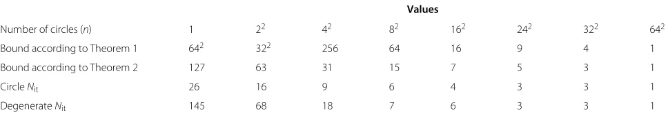
Table 1 Experimental validation of the theorems
Values
Number of circles (n) 1 22 42 82 162 242 322 642
Bound according to Theorem 1 642 322 256 64 16 9 4 1
Bound according to Theorem 2 127 63 31 15 7 5 3 1
CircleNit 26 16 9 6 4 3 3 1
DegenerateNit 145 68 18 7 6 3 3 1
overview of GPUs and, in addition to the basics, gives only those details that have great influence on the LS evolution. A function that can be executed on the GPU is called a kernel. Any call to a kernel must specify an NDRange for that call. This defines not only the number of work-items to be launched, but also the arrangement of groups of work-items to work-groups and work-groups to the NDRange. The dimensionality of a work-group can be one, two, or three.
Physically, the elementary computing element is the computing element. A few computing element together with a given amount of SDRAM, scheduling unit, and spe-cial function unit forms a computing unit (CU). A device consists of several CUs and a global memory (off-chip).
The experiments were done on an NVIDIA 780 GTX GPU. It has 12 CUs, 192 computing elements, and 48KB shared memory in each CU, and 3 GB global memory. The hosting PC runs on Intel core i7-2600 CPU @3.4 GHz with 8 GB system memory, the operating system is Debian with Linux kernel the GPU driver version is 325.15.
Experiments
Theorems 1 and 2 give upperbounds on the required num-ber of iterations (Nit). A practical proposal of this paper
is to construct configurations that have as low worst-case bounds onNitas feasible and can be computed efficiently
on many-core architectures. This scenario is presented through two case studies. The first one is on an Eye-RIS v1.3 VS that is a hardware implementation of the CNN-UM and the second one is on a GPU.
The whole image is covered with many-many small active fronts, and as a consequence, the intersection con-dition (∗p∩= ∅) is automatically fulfilled. During the case studies, the speedfieldFhas been very simple,+1 for the object region and−1 for the background regions.
A case study on CNN-UM
In subsection ‘CNN universal machine,’ a short overview was given on the CNN-UM. Now the details of the mapped algorithm are described. The perspective in this scenario is the precedence of locality which becomes increasingly important as the technology feature size decreases, and the delay together with power consump-tion of global communicaconsump-tion increases.
The mapped algorithm is based on the set theoretic description of the LS function. In addition toLinandLout
two other sets are defined.
Fin= {x∈D|φ(x) <0∧x∈/Lin} (7) Fout= {x∈D|φ(x) >0∧x∈/Lout} (8)
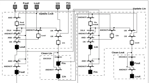
In other words, the neighbors of each point in these sets are in the same region as the point itself. Figure 2 shows
the universal machine on flows (UMF) diagram of the algorithm. It is a special flowchart description of the algo-rithms executable on CNN-UM so that it is complete and unique [20].
Templates AND, OR denote elementary logic, AND-NOT performs logic subtraction (Op1∧ ¬Op2), DIL4 and ERODE4 are the four connected dilatation and erosion (spatial logic). All templates are of the nearest neighbor kind. In the ‘Update Lout’ phase, foutmask is computed
first. It contains the points that are going to move outward.
foutmaskis used in three different ways. It is subtracted
(ANDNOT) from Lout, added (OR) to Lin and dilated
(DIL4, ANDNOT, AND) to generate its own outer neigh-bors. This is the new steppedLoutpart and the unchanged
parts are added with an OR operation. The resulting set is finalized as the newLout(black rectangle in Figure 2).
From the oldFoutthe newLoutis subtracted (ANDNOT)
to get the newFout(again, black rectangle in UpdateLout
phase). Finally, the modified Lin is added to Fin. In the
‘CleanLin’ phase, the mergedfoutmask,Lin, andFinis the
only input. The new Lin is the outer pixel layer of this
merged input. The newFin is obtained by a simple four
connected erosion whileLinis the result of a subtraction.
‘UpdateLin’ and ‘CleanLout’ are nearly identical, only the
input of the operations are switched, and another mask is used (finmask).
The algorithm is implemented on an Eye-RIS 1.3 VSoC. One step of the algorithm is performed in 400 to 440 µs on a QCIF image. It must be noted that the actual comput-ing is finished within 60 to 70 µs and the remaincomput-ing time (340 to 370 µs) is required for the data movement from the main memory of the Eye-RIS (on the Altea NIOS-II microprocessor) to the Q-Eye chip memory.
A case study on GPU
The evolution process is divided into two steps. The first one is the planner step and the second is the evolution step. The planner creates the so-called plan. It contains the position offsets of the 16×16 tiles that are calculated actually in the iteration step. The planner works on the indicator image. The indicator is a tiny image and each pixel of the indicator istrueif the corresponding tile on the input image shall be processed in this iteration and
falseotherwise. The size of the plan is calculated by local prefix-sum work-group wise, and global atomic addition is used to correctly determine the offset of the work-group within the plan. The source of the planner kernel is provided as Additional file 1.
Figure 2UMF diagram of LS evolution on CNN.Rectangles denote memories, bold short horizontal lines with capital operator names on the left denote template operations. Dashed lines indicate the phases corresponding to the four cycles of the Shi LSM. Black rectangles denote final forms of sets in that phase. Thin lines ending with arrows denote dataflow from memory to an operation, from an operation to an operation, or from an operation to a memory.
in the plan and writes the complete tile back to the global memory. First, each work-item calculates the new value of the pixel of the LS function. Then the neighbors of each pixel are updated as theswitch_out()andswitch_in() oper-ations require, and the active front is cleaned to maintain the two pixel width. If there is no activity inside the tile, then set the corresponding pixel of the indicator image to false. The boundary of the tile requires special care, namely, to properly update the corresponding neighbor-ing pixels of the LS function and the indicator. The source of the evolution kernel is provided as Additional file 2.
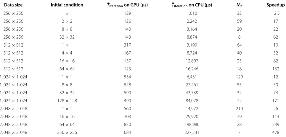
Table 2 shows execution time measurements of the work-efficient parallel algorithm on NVIDIA 780 GTX GPU compared to a baseline single-threaded implemen-tation on Intel core i7-2600 CPU. The execution time
was measured by the gettimeofday() C-function
which has microsecond resolution. The table specifies the image resolution, the initial condition configuration, and presents the mean of the execution time of an iteration on GPU, on CPU, and the speedup. The iteration time on the GPU contains the execution time of both kernel func-tions (planner, iteration). The two kernels evenly share the execution time in the case of conventional, sparse initial condition; however, in the case of dense iteration step, the
ratio of the evolution kernel can shift to 30:1 with respect to the planner.
Number of iterations
In the experiments more initial configurations were
tested. In each configuration, regions of and were
placed in a chessboard like pattern as it is showed in Figure 1A,B. Two sample objects are presented in Figure 1C,D that shall be detected. Additionally, the two objects represent the two object families: the degenerate and convex ones having worst-case bounds stated in the theorem 1 and 2.
Iteration results are presented in Table 1 together with the two different bounds of the given configuration. The number of iterations (Nit) was measured on the original
sequential algorithm of Shi and these values are presented in the table. It is below or equal to the worst-case bounds in every cases.
In the case of CNN-UM,Nitcoincides with the values
presented in the table, while in the case of GPU implemen-tation, Nit is consistently higher with one iteration. This
Table 2 Time measurements on NVIDIA GTX 780 GPU compared to Intel core i7 CPU
Data size Initial condition T¯iterationon GPU (µs) T¯iterationon CPU (µs) Nit Speedup
256×256 1×1 129 1,610 32 12.5
256×256 2×2 126 2,242 59 17
256×256 8×8 140 3,164 20 22
256×256 32×32 143 8,874 8 62
512×512 1×1 317 3,190 64 10
512×512 4×4 167 8,724 40 52
512×512 16×16 157 12,897 25 82
512×512 64×64 123 16,246 18 132
1, 024×1, 024 1×1 534 6,431 129 12
1, 024×1, 024 8×8 548 27,461 55 50
1, 024×1, 024 32×32 590 43,739 32 74
1, 024×1, 024 128×128 490 84,078 12 171
2, 048×2, 048 1×1 560 14,972 210 26
2, 048×2, 048 16×16 703 79,920 79 113
2, 048×2, 048 64×64 830 198,980 28 239
2, 048×2, 048 256×256 684 327,541 7 478
Presented results are the mean value of 100 runs.
cleaning process. This causes the additional iteration so it is not a violation of the theorems.
Validation
In this section, we compare the result of the exact numer-ical implementation and the Shi LSM for three different speed functions: mean curvature motion, Chan-Vese, and GAR. The quantitative comparison is made by the dice coefficient. Given the state of the two LS functions1and
2of the two different methods, the coefficient is defined
as
d(1,2)=
2Area(1∩2)
Area(1)+Area(2)
(9)
Its value is in the range of 0 and 1; 0 means complete difference and 1 means complete agreement.
Mean curvature flow
In this case, the speed function is defined as
F= −κ (10)
where κ is the (euclidean) curvature of the LS. It is the norm of the second derivative ofγ with respect to the (euclidean) arc length (κ = γss(s), s is the arc length
parametrization of the curve). Another possible, precise, and more easy way to calculate the curvature of an LS fromφis as follows:
κ =div grad ∇φ
∇φ (11)
This force term appears in almost every LS flow as a smoothing and regularizing term. The steady-state solu-tion is a circle with infinitesimal diameter. In practice, the object region vanishes. In this case, not only the steady state but the evolution itself is also investigated. This is an autonomous motion and does not have any control term from an external image.
The details of the numerical approximation are as fol-lows. The LS function φ is a signed distance function. It was recalculated after every 30 iterations. The time (Tmaximum) run to 800 units. The time step (t) size has
been set to 0.4. The curvature has been calculated from the LS function from Equation 11.
In the case of the fast LS evolution, the curvature was calculated according to the work Merriman, Bence, and Osher (MBO) [23,24], namely, byG⊗φ, whereGis a 2D gaussian of a given variance.
Figure 3 shows the test initial condition for mean curva-ture motion and the state of the evolution after 20, 40, 60, and 80 iterations of the fast LS evolution.
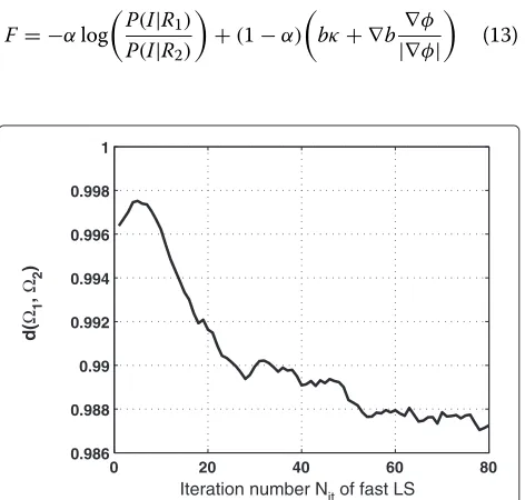
Figure 4 shows the dice coefficient between the first 80 steps of the fast LS evolution and the corresponding state of the numerical approximation.
Chan-Vese flow
This method was proposed in [6] and its speed term is defined as
F=μκ−λ1(c1−I)2+λ2(c2−I)2 (12)
The parameters are set as follows:μ= 1,λ1 = 0.8,λ2=
Figure 3Comparison of mean curvature evolution of PDE approximation and fast LS evolution.This shows the initial condition and evolution of fast LS (white line) and numerical PDE approximation (black line).(A)Test initial condition for validation of mean curvature motion fast LS evolution against numerical PDE approximation. The test region contains positive, negative, and zero curvature regions and singularities as well. (B)State of evolution fast LF atNit=20 and PDE approximation atT=56.8.(C)State of evolution fast LF atNit=40 and PDE approximation at
T=190.8.(D)State of evolution fast LF atNit=60 and PDE approximation atT=405.6.(E)State of evolution fast LF atNit=80 and PDE
approximation atT=706.8.
c1 = 0.5 andc2 =0 are simply the means of pixel
inten-sities inside and outside the zero LS. The artificial time parameter runs to 180 units, the time step is 0.5 units. The total number of iterations are 360. The initial condi-tion is 25 circles arranged uniformly in five rows and five columns each with diameter 27 pixels. The LS function (signed distance) is recalculated in each 30 iterations for the numerical solution. The initial condition is 5×5 cir-cles each with diameter 27 pixels. The steady states of the two Cahn-Vese evolutions are shown in Figure 5A. The dice index of the two states is 0.998.
Geodesic active regions flow
This method was proposed in [7]. This method combines boundary and region-based information to segment an image. In this method, the pixel intensities are modeled with a GMM. The speedfield is as follows:
F= −αlog
P(I|R1) P(I|R2) +(
1−α)
bκ+ ∇b ∇φ
|∇φ| (13)
0 20 40 60 80
0.986 0.988 0.99 0.992 0.994 0.996 0.998 1
Iteration number Nit of fast LS
d(
Ω1
,
Ω2
)
Figure 4Dice index of mean curvature evolution.1is the state
of the fast LS evolution, and2is the state of the numerical solution.
The similarity between the two states is very high.
where R1andR2 are the regions to be separated,b is a
strictly decreasing function of boundary probability, and α is a balancing constant. In our caseα = 0.3, andbis defined as follows:
b= 1
1+ ∇G⊗I (14)
HereGis a 2D gaussian withσ = 3. The GMM
param-eters are calculated from the image histogram with a recursive expectation maximization algorithm. The arti-ficial time runs to 6 units, the time step is 0.02 units. The total number of iterations are 300. The LS function (signed distance) is recalculated in each 30 iterations for the numerical solution. The initial condition is the same as in the case of Chan-Vese evolution, 5×5 circles each with diameter 27 pixels. Steady states are shown in Figure 5B. The dice index of the two states is 0.998.
Discussion
In this paper, given our investigation of the initial condi-tion and the required number of iteracondi-tions as a funccondi-tion of it, we presented two bounds on the required number of iterations of an LS evolution. The bounds were proven theoretically and validated experimentally with the origi-nal algorithm and also with two different mappings of the algorithm on many-core machines (GPU, CNN-UM). The bounds depend only on the initial configuration of the LS function. The many-core realizations required not only a very small number of iterations less than or equal to the bounds, but the execution of an iteration was also fast (see Table 2 for detailed measurement data).
Figure 5Validation of fast LS evolution.(A)CV and(B)GAR flow. Red corresponds to the numerical PDE solution while blue corresponds to the fast LSM. The two curves are nearly the same and the dice index is 0.998 in both cases.
significant speedup compared to the sparse initial condi-tion in all cases since our proposed dense initial condicondi-tion together with the algorithm utilizes the properties of the underlying architecture. Therefore, greater performance gain can be achieved on GPU if dense initial condition is used.
A great property of the results is the scalability. This is true for the performance as a function of cores and for the number of iterations as a function of size of the dis-joint active fronts. Considering the chessboard-like initial configuration with increasingly finer regions, the general bound is proportional to the area of the regions and the convex bound is proportional to the half perimeter of the regions. This is changed in three dimensions to the vol-ume of region in the case of general bound and half of the longest perimeter of the volume in the case of a convex bound.
The assumption on F is stronger in Theorem 1 than
the one that was given in the convergence analysis in [2]. In the examples presented there, our stronger assumption stands for at least one of the regions∗,∗. However, there may be cases when for a short period of iterations the sign of F changes. Typically, this is the case when inside the true object region, the actual state of the LS function contains a concave background region with high negative curvature. In these cases, the curvature-based term can be greater than the region term (the pixel-intensity-based terms), but this is a temporary effect. As soon as the local concavity is vanished, the region term
becomes again greater and the sign of F changes back.
Furthermore, as it was declared in the introduction, the construction of the speedfield and its components is out of the scope of this paper. Additionally, the validations indi-cate that the method convergesde factoto the same state as the exact numerical solutions.
The fact that the active front of the initial condition cov-ers the whole image has a special consequence, namely,
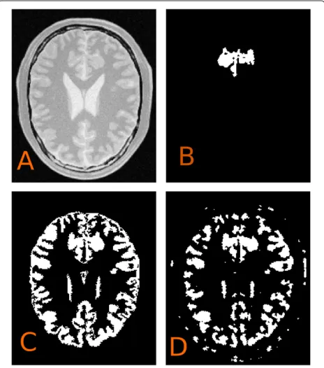
separate, disjoint regions of the same object or multiple target objects can be found automatically without user interaction. For example, the grey matter of the brain on an MRI slice is disconnected and may be composed of 8 to 20 disjointed regions on the given slice. The problem of detecting all regions is greatly simplified with our dense
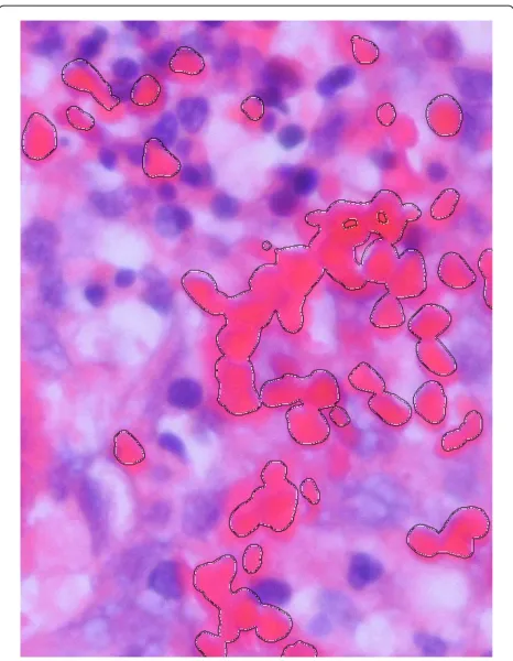
Figure 7Histology image from the skin.
initial condition. Similarly, the selected group of cells on a histology image shows this property as well. Additionally, histology images can be extremely large (2 to 30 Mpixel), and the performance gain of our proposed method (initial condition together with the parallel algorithm) becomes more expressed on larger images. A conventional sparse initialization can easily fail this task, with wrongly cho-sen initial condition, see for instance the initialization and evolution of a gold standard LS implementation of [25], which is a widely used framework for medical image segmentation and analysis.
Figures 6 and 7 show an example. The evolution from a single-circle initial condition is presented on Figure 6B, while our result is presented in Figure 6C,D. It demon-strates its potential and it may be an initial condition for fine-tuning the segmentation with another method. Of course, the dense iteration may have the drawback of increased false-positive rate, for example see Figure 6D where the evolution runs with slightly different parame-ters, but this could be handled with more sophisticated speed functions or buildinga prioriinformation into the initial condition. Figure 7 shows a histology image from the skin, where one class of cells is to be segmented.
It must be emphasized that the case studies presented here are not necessarily optimal mappings of the Shi LS
evolution by any means. The purpose of presenting them is twofold: (1) to highlight the advantage of the proposed initial condition concept especially on those machines and (2) to give a proof of concept mapping of this fast evo-lution on two totally differently organized (virtual and physical) many-core machines.
Conclusions
To automatically detect segment object on an image or on a region of it, the LS-based algorithms are feasible tools. In this paper, it was shown theoretically and experimentally through two case studies that the initial condition plays an essential role in decreasing the execution time. It must be emphasized that this is only validated on many-core architectures where the computations can be distributed among the cores. Furthermore, based on the initial condi-tion configuracondi-tion, two worst-case bounds were given on the required number of iterations depending on the con-vexity of the object to be found. The bounds are proven theoretically and validated experimentally. Additionally, the execution time of one iteration was measured on both architectures. It was below 70+370 µs on the Eye-RIS sys-tem handling a QCIF image (where 70 µs is the processing time and 370 µs is the outer memory delay). The timing results of the GPU is presented in Table 2 in details. In the case of the proposed dense initial condition on GPU, there is a significant speedup compared to the sparse ini-tial condition in all cases since our dense iniini-tial condition together with the algorithm utilizes the properties of the underlying architecture. Therefore, greater performance gain can be achieved (up to 18 times speedup compared to the sparse initial condition on GPU).
The results and tools presented in this paper provide a method to efficiently map LS algorithms on many-core architectures and ensure bounds on the execution time through the two theorems.
Additional files
Additional file 1: The OpenCL source of the planner kernel.
Additional file 2: The OpenCL source of the evolution kernel.
Competing interests
The authors declare that they have no competing interests.
Acknowledgements
This research was supported by the European Union and the State of Hungary, cofinanced by the European Social Fund in the framework of TÁMOP 4.2.4.A/1-11-1-2012-0001 (National Excellence Program). The support grants TÁMOP-4.2.1.B-11/2/KMR-2011-0002 and TÁMOP-4.2.2/B-10/1-2010-0014 are also gratefully acknowledged. The authors would like to thank Ádám Rák for his help and suggestions.
References
1. JA Sethian,Level Set Methods and Fast Marching Methods: Evolving Interfaces in Computational Geometry, Fluid Mechanics, Computer Vision,
and Materials Science. (Cambridge University, New York, 2000)
2. Y Shi, W Karl, A real-time algorithm for the approximation of
level-set-based curve evolution. IEEE Trans. Image Process.17(5), 645–656 (2008) [http://ieeexplore.ieee.org/lpdocs/epic03/wrapper.htm? arnumber=4480128]
3. D Adalsteinsson, JA Sethian, A fast level set method for propagating interfaces. J. Comput. Phys.118(2), 269–277 (1995) [http://www. sciencedirect.com/science/article/pii/S0021999185710984]
4. D Peng, B Merriman, S Osher, H Zhao, M Kang, A PDE-based fast local level set method. J. Comput. Phys.155(2), 410–438 (1999) [http://www. sciencedirect.com/science/article/pii/S0021999199963453] 5. G Sapiro,Geometric Partial Differential Equations and Image Analysis.
(Cambridge University, New York, 2001)
6. T Chan, L Vese, Active contours without edges. Image Process. IEEE Trans.
10(2), 266–277 (2001)
7. N Paragios, R Deriche, Geodesic active regions: a new framework to deal with frame partition problems in computer vision. J. Vis. Commun. Imag. Rep.13(1–2), 249–268 (2002) [http://www.sciencedirect.com/science/ article/pii/S1047320301904754]
8. N Joshi, M Brady, Non-parametric mixture model based evolution of level sets and application to medical images. Int. J. Comput. Vis.88, 52–68 (2010) [http://dx.doi.org/10.1007/s11263-009-0290-5]
9. L Bertelli, S Chandrasekaran, F Gibou, BS Manjunath, On the length and area regularization for multiphase level set segmentation. Int. J. Comput. Vis.90(3), 267–282 (2010) [http://www.springerlink.com/index/10.1007/ s11263-010-0348-4]
10. G Sundaramoorthi, A Yezzi, A Mennucci, G Sapiro, New possibilities with Sobolev active contours. Int. J. Comput. Vis.84, 113–129 (2009) [http://dx.doi.org/10.1007/s11263-008-0133-9]
11. AE Lefohn, JE Cates, RT Whitaker,Interactive, GPU-based level sets for 3D
segmentation. ed. by Ellis RE, Peters TM, Medical Image Computing and
Computer-Assisted Intervention - MICCAI 2003, Lecture Notes in Computer Science. vol. 2878 (Springer, Berlin Heidelberg, 2003) pp. 564–572, [http://dx.doi.org/10.1007/978-3-540-39899-8_70] 12. M Roberts, J Packer, MC Sousa, JR Mitchell, inProceedings of the
Conference on High Performance Graphics. A work-efficient GPU algorithm
for level set segmentation (ACM, New York, 2010), pp. 123–132 13. O Sharma, Q Zhang, Q Anton, C Bajaj, in2010 IEEE Conference on,
Computer Vision and Pattern Recognition (CVPR). Multi-domain, higher
order level set scheme for 3D image segmentation on the GPU (San Francisco, 13–18 June 2010), pp. 2211–2216
14. LO Chua, L Yang, Cellular neural networks: applications. Circuits Syst. IEEE Trans.35(10), 1273–1290 (1988)
15. G Cserey, C Rekeczky, P Földesy, PDE based histogram modification with embedded morphological processing of the level-sets. J. Circuits, Syst Comput.12(04), 519–538 (2003)
16. C Rekeczky, T Roska, inProceedings of the European Conference on Circuit
Theory and Design, Volume 2. Calculating local and global PDEs by
analogic diffusion and wave algorithms (Helsinky University of Technology, Espoo, 2001), pp. 17–20
17. D Hillier, Z Czeilinger, A Vobornik, C Rekeczky, Online 3-D reconstruction of the right atrium from echocardiography data via a topographic cellular contour extraction algorithm. Biomed. Eng. IEEE Trans.57(2), 384–396 (2010)
18. Y Shi, WC Karl, inProceedings on IEEE International Conference on Acoustics,
Speech, and Signal Processing (ICASSP’05), vol. 2. A fast level set method
without solving PDEs (Philadelphia, 18–23 March 2005, 2005), pp. 97–100 19. Y Shi, Object based dynamic imaging with level set methods. PhD Thesis,
Boston University College of Engineering 2005
20. LO Chua, T Roska, PL Venetianer, The CNN is universal as the Turing machine. Circuits Syst. I: Fundam. Theory Appl. IEEE Trans.40(4), 289–291 (1993)
21. NVIDIA:CUDA C Programming Guide2011. [https://developer.nvidia.com/ cuda-toolkit-archive]. Accessed 23 January 2012
22. OpenCL specification 1.12011. [http://www.khronos.org/opencl/].
Accessed 1 April 2012
23. B Merriman, J Bene, S Osher, inComputational Crystal Growers Workshop. Diffusion generated motion by mean curvature. Edited by Taylor J, (Providence, RI 1992) pp.73–83.
24. B Merriman, JK Bence, SJ Osher, Motion of multiple junctions: a level set approach. J. Comput. Phys.112(2), 334–363 (1994). [http://www. sciencedirect.com/science/article/pii/S0021999184711053] 25. The insight toolkit 2012. [www.itk.org]. Accessed 20 November 2012
doi:10.1186/1687-6180-2014-30
Cite this article as:Tornai and Cserey:Initial condition for efficient mapping
of level set algorithms on many-core architectures.EURASIP Journal on Advances in Signal Processing20142014:30.
Submit your manuscript to a
journal and benefi t from:
7Convenient online submission
7Rigorous peer review
7Immediate publication on acceptance
7Open access: articles freely available online
7High visibility within the fi eld
7Retaining the copyright to your article