F U L L P A P E R
Open Access
Observed geomagnetic induction effect on
Dst
-related magnetic observations under different
disturbance intensities of the magnetospheric
ring current
Dan Xu
*, Huaran Chen and Mengtan Gao
Abstract
Based on the spherical harmonic expansion of geomagnetic disturbance observed on the mid-latitude surface of the Earth, external and internal field separation is conducted in which the external component is magnetic disturbance caused by the magnetospheric ring current and the internal component is that raised by the correspondingly induced currents within the Earth. The objectives are to evaluate the influences of the induced internal field on the surface magnetic observations and to reveal the response performance of internal geomagnetic induction under different strengths of magnetospheric ring current fluctuations for better understanding of the disturbance storm time (Dst) index variations. The results show that the ratio of the internal component to surface observation does not remain constant in storm time. During the main phase of the storm, the ratio variation follows the pattern of logarithmic growth with storm evolution up to the top value at theDst-minimum; then, the ratio slowly decreases in the long recovery phase. Multiple small logarithmic growths are superimposed on the traces of internal ratios, corresponding to temporary ring current intensification during the storm main phase and amplifying the effect of this intensification on surface magnetic observations. With the intensification of magnetospheric storms from the level of (−200nT,−100nT) to (−300nT,−200nT) and (−500nT,−300nT) classified with theDst-minimum, the top value of the ratio averaged for each storm group in the superposed epoch analysis method increases from the value of 0.295 ± 0.014 to 0.300 ± 0.016 and 0.308 ± 0.015, respectively. It is demonstrated that the geomagnetic induction exceeds the linear relation with the intensification of the external field, which is physically reasonable and coincident with the Faraday’s law of induction. Due to the effects of high induction of the oceans and lateral heterogeneity of electric conductivity distribution in the upper mantle of the Earth, the geomagnetic induction and its contribution to surface geomagnetic disturbance vary significantly among observatories. This factor should be considered in the research of magnetospheric current systems.
Keywords:Geomagnetic storms; Geomagnetic induction;Dstindex
Background
Geomagnetic variations on the Earth’s surface with time scales of seconds to a year primarily result from dynamic processes in the ionosphere, magnetosphere, and helio-sphere. Geomagnetic storms, the most severe magneto-spheric disturbances, are caused by intensified energy and momentum injection when the magnetosphere encounters fluctuated solar wind structures such as cor-onal mass ejections (CMEs). The representative feature
of such storms is a significantly intensified equatorial ring current encircling the Earth westward, which is caused mostly by the drifting of energetic particles filling the inner magnetosphere from 2 to 9 RE. The ring current-induced magnetic field is opposite the Earth’s main field at the equator and leads to remarkable de-pression of magnetic observation during storm time (Gonzalez et al. 1994). The symmetric part of geomag-netic disturbance on the low-latitude surface is tracked and quantified by the disturbance storm time (Dst) index (Sugiura 1964) derived from variations of the horizontal components of geomagnetic observations at four
low-* Correspondence:[email protected]
Institute of Geophysics, China Earthquake Administration, Beijing 100081, China
latitude geomagnetic observatories (Sugiura and Kamei 1991). TheDstvariation is conventionally interpreted as a proxy of the symmetric ring current.
Recent research has indicated that geomagnetic distur-bances due to the estimated ring current derived from both in situ magnetospheric particle measurements and simulated magnetospheric particle distributions have all underestimatedDstvariation (e.g., Hamilton et al. 1988; Turner et al. 2001; Liemohn and Jazowski 2008). In fact, temporal variation of the magnetospheric ring current can excite induced currents in the Earth, which give rise to the secondary magnetic field and lead to further mag-netic disturbances observed on the Earth’s surface. As a result, the observed surface magnetic disturbances con-tain a contribution of the induced magnetic field origin-ating from internal regions of the Earth responding to time variation of the magnetospheric ring current.
The induced magnetic disturbances from the Earth’s interior sensed by geomagnetic observatories have been utilized to reveal mantle electrical conductivity struc-tures since this method was implemented (e.g., Banks 1969; Schultz and Larsen 1990; Constable 1993; Olsen 1999; Kelbert et al. 2009; Khan et al. 2011). This tech-nique has been valued as the most important method for studying mantle conductivity. Even for geomagnetic satellites orbiting at an altitude of 450 km, the induced magnetic field still can be detected and used for mantle studies (Constable and Constable 2004; Martinec and McCreadie 2004; Kuvshinov and Olsen 2006; Püthe 2013a, b; Velímský 2013). For convenience, the mag-netospheric currents are referred to as external sources, and the correspondingly induced currents and magnetic fields within the Earth are referred to as internal sources with respect to the magnetic field observed on the sur-face of the Earth.
The spatial configurations and fluctuating periods of external source currents in the magnetosphere and iono-sphere, the conductivity distribution features inside the Earth, and the locations of magnetic probes are all key elements for the measurement of induction effects within the Earth (Mareschal 1986). The internal propor-tion could account for one-third of the magnetic obser-vation in an idealized situation such that the Earth is perfectly conducting and the involved order of the spherical harmonic for external current configuration is onlyn= 1 (Price 1967). Häkkinen et al. (2002) examined magnetic observations from Dst standard observatories for 12 storms ranging from−76 to−216 nT in 1997 and 1998; the average internal contribution toDstat roughly 30% during the storm main phase decreased to about 20% during the recovery phase. For the actual magnetic observations, the internal contribution is less than that in the idealized case, but it is still remarkable and de-serves careful investigation.
From the condition of Dst variation, the magneto-spheric disturbance and the ultimate source in solar wind can be approximately evaluated through analysis of works that differentiate solar wind disturbance struc-tures and identify the solar wind sources of geomagnetic storms with different intensities (Gonzalez et al. 2011). Since the Dst index can be conveniently obtained from geomagnetic observatories, Dst variation is the most common and efficient indication of magnetospheric dis-turbances, particularly for geomagnetic storms. Extreme geomagnetic storms can adversely affect the instruments of satellites in the inner magnetosphere and surface power systems; therefore, Dstindex prediction is essen-tial for satellite exploration and daily human life. Solar wind plasma and interplanetary magnetic field measure-ments ahead of the Earth’s bow shock are commonly used as basic input parameters and are sometimes the only input parameters (e.g., Temerin and Li 2002, 2006) used to predict Dst variations. These predictions are mostly acceptable if the departure is ignored to some ex-tent because solar wind disturbances are the most im-portant driving sources for magnetospheric disturbance. However, accuracy in space physics and Dst prediction in fact requires determination of the exact contribution of internal induced current toDstdepression with differ-ent levels. Therefore, the objective of this study is to de-termine whether any differences in internal contribution to the Dst index occur in geomagnetic storms with dif-ferent intensities.
Methods Dstcalculation
Dst is an hourly index calculated from the horizontal component of four geomagnetic observatories at middle latitudes: Honolulu (HON, geomagnetic colatitude and longitude: 68.45°, 270.73°), San Juan (SJG, 62.31°, 6.87°), Hermanus (HER, 123.99°, 85.14°), and Kakioka (KAK, 62.31°, 209.58°), which are located with sufficient differ-ence from both auroral and equatorial electrojets and are evenly distributed in longitude (Sugiura and Kamei 1991).
In this paper, we adopt the basicDstcalculation method of Sugiura and Kamei (1991) following Häkkinen et al. (2002) to acquire the disturbed magnetic component by eliminating the baseline of secular variation due to the Earth’s main magnetic field and its long period variation, crustal magnetic field, and the field from stable external current systems at the quiet time of the magnetosphere and ionosphere. We then subtract the solar quiet daily variationSq. The remnant is considered to be a
The baseline of each magnetic component is com-puted by first calculating the annual mean value with the five quietest days of each month in the considered year and the preceding years. Then, we conducted a second-order polynomial fit to the annual mean values to obtain the baseline for each day.
Bbase
x;y;z ¼ax;y;zþbx;y;zTþcx;y;zT2 ð1Þ
This data process procedure is conducted for all three components of surface magnetic observations, Bx, By, and Bz, in local Cartesian coordinates. In the standard
Dst derivation method, only the horizontal component of the field is considered. However, because theBz com-ponent is indispensable for studying the interior electric structures of the Earth, the radial component is equally processed in our research following the same procedure as that used for the horizontal component.
Sugiura and Kamei (1991) expanded theSqas a double Fourier series in local time Tand month number M to statistically fitSqcurves for each day in 1 year.
SqðT;MÞ ¼
In equation (2), we take the same maximum value for
mandnas that reported by Häkkinen et al. (2002). The coefficientsAmn, αm, andβnare determined by comput-ing oneSqcurve for each month with the average of the five quietest days in the month.
The disturbed field accounting for Dst variations at each observatory is then obtained from the equation
Bx;y;z¼Bobsx;y;z−Bbasex;y;z−Sqð ÞT . Then, the Dst index is
de-rived from the four standard stations through the formula:
Dst Tð Þ ¼X4n¼1Hcosnð ÞϑT
n ; ð3Þ
where Hstands for the disturbed horizontal field andϑ is the geomagnetic latitude at each station.
Separation of internal and external fields
The Dst-related magnetospheric ring current possesses the predominantP0
1 spherical harmonic geometry in
mid-latitude regions (Banks 1969). Moreover, the Dst-related magnetic disturbances can provide an estimation of in-ternal and exin-ternal coefficients of Dst variations through spherical harmonic expansion of the disturbed field. Due to the consideration of conciseness in the physical cept, the reference frame of the disturbed field is con-verted from a geographic to geomagnetic coordinate system on the surface of the Earth.
The region between the Earth’s surface and the iono-sphere is generally current source-free, in which the
magnetic field is conservative or curl-free and can thus be expressed as the gradient of a scalar potential (Lorrain and Corson 1970; Jackson 1998; Backus et al. 1996; Sabaka et al. 2010), known as potential magnetic field, as shown in equation (4).
⇀
B¼−∇V ð4Þ
Additionally, based on Maxwellian equations, the mag-netic field vector must be solenoid, which implies:
∇2V ¼0: ð5Þ
The potentialVis harmonic, and this Laplace equation can be solved easily in a geomagnetic spherical coordin-ate system (r,θ, ∅) where r is the radial distance from the center of the Earth, θ is the geomagnetic colatitude angle ringing from 0° at geomagnetic north pole to 180° at the south pole, and∅is the longitude angle expressed as a spherical harmonic expansion of associated Legen-dre polynomials Pml , with Schmidt quasi-normalized spherical harmonic coefficients iml eml representing the internal and external magnetic fields:
V rð;θ;ϕÞ ¼aX∞l¼1Xlm¼−1 im
whereais the Earth’s radius. Keeping only theP0 1
contri-bution forDst-related disturbances under the assumption of symmetrical ring current (Constable and Constable 2004; Kuvshinov and Olsen 2006),
V rð ;θÞ ¼a i0
By using equation (7), the magnetic field vector⇀Bof disturbed field as componentsBr,Bθ, andB∅in the geo-magnetic spherical coordinate system and thus the sym-metric geomagnetic disturbance can be expressed as:
Br¼ −e01þ2i01
The Bθ component represents the southpole-directed
horizontal component of Dst-related magnetic field dis-turbance in the geomagnetic spherical coordinate system, the Br component is the same as the disturbed Bz
approximately. Then, the externale0
1and internali01
coeffi-cients can be resolved directly from equation (8).
e0
Then, the contribution rates of the external field (Be) and internal field (Bi) to the symmetrical
dis-turbed field (Bθ) on the surface observatories can be
expressed as:
Then, the external contribution to the Dst index can be derived from the external partBeof each station and
equation (3).
Assuming that the interior of the Earth is a perfect electric conductor, in which the fluctuated period of ex-ternal field should be sufficiently fast and the interior conductivity within the Earth should be sufficiently large according to the penetration depth δ¼pffiffiffiffiffiffiffiffiffiffiffiffiffiffiffiffiffiT=πμ0σ of the magnetic field, internal currents would be induced to prevent any external field from entering the con-ductor, and the radial magnetic component measured on the surface will vanish. This means that internal induced currents have excited magnetic fields in which radial component cancels the radial part of the external field. In equation (10), when the radial component of the magnetic field is zero, the internal part is one-third of the horizontal component, which coincides with the in-ference of Price (1967).
Results and discussion
We adopted the geomagnetic observations of 68 intense geomagnetic storms (Dst≤ −100 nT) at four Dst geo-magnetic observatories recorded from 2000 to 2013. The standard method for Dst index derivation reported by Sugiura and Kamei (1991) and the internal/external field separation technique introduced in the last section were utilized. The objectives were to investigate the observa-tional performances of geomagnetic induction from in-ternal induced currents of the Earth and the possible divergence of their contributions to Dstvariations with different intensities to improve the accuracy in Dst prediction.
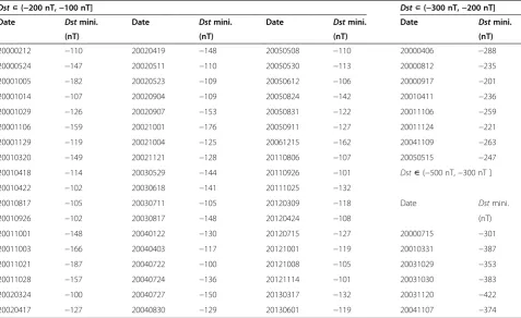
The selected storms were divided into three classes ac-cording to their intensities, as shown in equation (12) and Table 1.
G1:Dst∈ −ð 200nT;−100nT G2:Dst∈ −ð 300nT;−200nT G3:Dst∈ −ð 500nT;−300nT
ð12Þ
These storms literally belong to intense storms accord-ing to the classification of (Gonzalez et al. 1999), of which 80% could have been caused by coronal mass ejection (CME; Xu et al. 2009). For CME, the sheath re-gion and the magnetic flux rope with a southward inter-planetary magnetic field after high-speed interinter-planetary shock is the dominant source responsible for the pres-ence of the main phase of intense storms, particularly with significant Dst depression. Consequently, the main phases of intense storms led by CMEs have an average duration of about 10 h, which is obviously shorter than the average main-phase duration of about 27 h for weak storms led by interplanetary corotating interaction re-gions (CIRs; Hutchinson et al. 2011). For geomagnetic induction from internal induced currents, the variation period of external sources is a critical issue for determin-ing the penetration depth under certain observatory con-ditions. Within this depth of interior layers, the actual heterogeneity of electric conductivity distribution is re-sponsible for the discrepancy of electric and magnetic in-duction affecting surface observations; beyond this depth, the external magnetic signal is generally shielded. Moover, for actual Earth conditions, the phase lag of the re-sponse relation between the induced internal and external source field depends on the varying periods of the external source field. However, different from intense storms, nearly 40% of storms withDstabove−100 nT could be re-sulted by CIRs, thus possessing a much longer storm main phase. Therefore, only the data of intense storms were adopted in this research under the assumption that they all have gone through nearly the same time scale of main phase duration. In such cases, similar penetration depth at a certain observatory may be guaranteed for all storms.
and the recovery phase, respectively, according to typical durations of intense storm developments. The data for each storm phase were shifted to fit these durations to superpose the epochs of all selected storm phases. The onset of the main phase and theDst-minimum were the common reference times for this superposition. The on-set of the main phase was chosen as the point followed by sudden drops in Dst value, and the Dst-minimum was the start of the recovery phase.
For each storm, the baseline of secular variation was removed from the original magnetic observation in each station. The field derived from the Sq current system
was subsequently eliminated from the remnant. Next, the residual field was considered asDst-related magnetic variation originating from disturbed magnetospheric current systems and the induced currents in the Earth. These Dst-related disturbances were then projected to the geomagnetic spherical coordinate system on the Earth’s surface (Br,Bθ,B∅) to conduct the separation
pro-cedure of internal and external components based on equation (9) for each storm at each station.
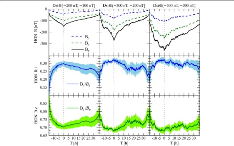
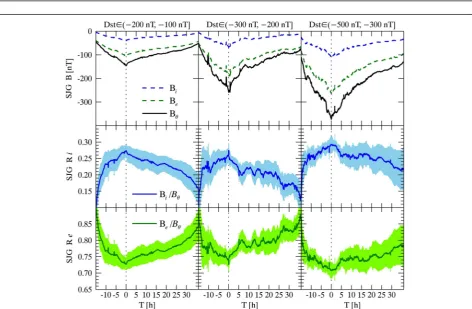
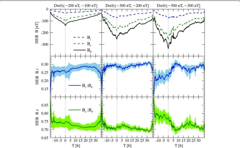
With the separated internal and external fields, the pe-riods of the main and recovery phases of storms were extracted to obtain the mean values for each storm cat-egory by performing SEA. Figures 1, 2, 3, and 4 demon-strate the SEA results obtained at HON, KAK, SJG, and HER stations. The dashed lines in the upper panels show
the storm time variations of internal partBiand external
partBeout of the disturbed horizontal field Bθof dipole
symmetry; Bθ fields appear as solid lines. The bottom
two ratio components illustrate the traces of field ratios (Ri=Bi/Bθ, Re=Be/Bθ) over the period of storm
evolu-tion. Blue and green lines represent internal and external field ratios, respectively, as indicated by the graph legends. The ambient margins around the curves in the ratio panels illustrate the standard deviations of the SEA process, which measure the spread of datasets and the dispersion from the SEA mean values. In each panel, the horizontal axis measures time in hours, and theDst -mini-mum is marked as the zero point demonstrated by the black vertical dotted line, which indicates the end of the storm main phase and the beginning of the recovery phase during the evolution of the geomagnetic storm. The start point of the time axis shows the onset of the storm main phase. The three columns in the graph show SEA results for G1, G2, and G3 storm levels, respectively.
Figure 1 presents the SEA mean values of magnetic fields and their ratios at HON station. According to the upper three panels of magnetic field components, it is obvious that internal and external fields followed the same variation pattern as that exhibited by the changes in the surface dipole symmetric field Bθ during the
storm time, in which the fields significantly dropped from the onset point during the storm main phase until
Table 1 Adopted intense geomagnetic storms from 2000 to 2013
Dst∊(−200 nT,−100 nT] Dst∊(−300 nT,−200 nT]
Date Dstmini. Date Dstmini. Date Dstmini. Date Dstmini.
(nT) (nT) (nT) (nT)
20000212 −110 20020419 −148 20050508 −110 20000406 −288
20000524 −147 20020511 −110 20050530 −113 20000812 −235
20001005 −182 20020523 −109 20050612 −106 20000917 −201
20001014 −107 20020904 −109 20050824 −142 20010411 −236
20001029 −126 20020907 −153 20050831 −122 20011106 −259
20001106 −159 20021001 −176 20050911 −127 20011124 −221
20001129 −119 20021004 −125 20061215 −162 20041109 −263
20010320 −149 20021121 −128 20110806 −107 20050515 −247
20010418 −114 20030529 −144 20110926 −101 Dst∊(−500 nT,−300 nT ]
20010422 −102 20030618 −141 20111025 −132
20010817 −105 20030711 −105 20120309 −118 Date Dstmini.
20010926 −102 20030817 −148 20120424 −108 (nT)
20011001 −148 20040122 −130 20120715 −127 20000715 −301
20011003 −166 20040403 −117 20121001 −119 20010331 −387
20011021 −187 20040722 −100 20121008 −105 20031029 −353
20011028 −157 20040724 −136 20121114 −101 20031030 −383
20020324 −100 20040727 −150 20130317 −132 20031120 −422
achieving the minimum value and gradually recovering. For the G1 category in the left column of the graph, the internal ratio Ri shows rapid growth in the duration of
the main phase in a logarithmic manner and slowly de-creases after reaching the top value at the point of the
Dst-minimum. The standard deviation was smaller at the points around theDst-minimum than regions before and after, suggesting that the SEA mean value estimation is statistically somewhat more reliable in the data points around theDst-minimum. The external ratiosRewere the
complete reverse of the internal ratios. The field ratios illustrate that for the surface magnetic observations, the ra-tio of the external fluctuara-tion part caused by the magnetic ring current decreased whereas the ratio of the internal in-duced field increased during the storm main phase, reach-ing extreme values at the Dst-minimum before achieving slow recovery. For the sake of simplicity, the physical pa-rameters of the magnetic fields and ratios referred in the SEA results all represent their SEA mean values.
As the storm levels intensified, the traces of the Bθ
field clearly showed multiple small intensifications dur-ing the main phases, with one obvious dip for the G2 category in the middle column and three dips for G3 in the right column of the graph. These small dips mainly
resulted from multiple temporarily intensified injections of charged particles into the magnetic ring current or pos-sible energization mechanisms of ring current particles during the storm main phase. Clearly, larger storms nor-mally contain more temporarily intensified injections of charged particles. The internal external part of the mag-netic field and their contribution ratios all showed evi-dence of intermittent intensification. Moreover, for each temporary intensification of the external field, the internal ratio experienced a sudden increase correspondingly, as shown in the lower panels of the graph. For each category, the maximum of theRi mean value was 0.298 ± 0.012 at
the Dst-minimum for G1 and increased to 0.325 ± 0.006 and 0.324 ± 0.015 for G2 and G3, respectively. During the main phase of G2 and G3, the values ofRiwere
remark-ably larger than those of G1, even in the recovery phase. At KAK and SJG stations, the variation trend of mag-netic field components and their ratios nearly main-tained the same values as HON for each category, although the significant temporary intensifications were lower than those of HON during the main phases. For the G1 category, the external fieldBenearly maintained
the same values among allDststations, which somewhat proves the polar-axis symmetry of the magnetic ring Figure 1Superposed epoch analysis (SEA) results of magnetic components and the related ratios during the storm time at HON. The SEA mean values of the dipole symmetrical horizontal components (Be) of geomagnetic observations in geomagnetic spherical coordinate,
external fields (Be) arising from the disturbance of the magnetospheric ring current and internal induced fields (Bi), and the internal and external
Figure 3Superposed epoch analysis (SEA) results of magnetic components and the related ratios during the storm time at SJG.
current under the storm level of the G1 category. For G2 and G3 categories, however, the Be values were
slightly different. This difference may have been partly caused by the much less statistical cases in G2 and G3 categories and unavoidable missing data. At KAK station for G3, although the top value of Ri (0.308 ± 0.009) was
just equal to that of the G1 category (0.307 ± 0.013), the value of Ri was still larger than that G1 at the points
during the main and recovery phases. At SJG station, the top value ofRiwas 0.273 ± 0.017 in G1 and above 0.292 ±
0.023 in G3, showing an obvious increase. The Ri values
during the main and recovery phases in G3 were on aver-age larger than those of G1 and G2.
For HER station, the tendency ofRivariation remained
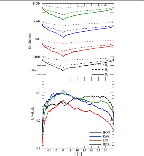
the same for three storm groups. The values were un-usually larger and reached the top value in the recovery phase, which differs in pattern from that of HON, KAK, and SJG. This situation of HER is similar to that re-ported by Häkkinen et al. (2002), in which the internal contribution is very small in the storm main phase but is larger and nearly remains constant in the recovery phase. The upper panel in Figure 5 shows the averaged value of the Bθ field and its internal and external parts
over all selected storms in each station, and the lower panel illustrates the corresponding variations of the Ri
values. It is clear that the value ofRiat KAK was slightly
larger than that at HON during the main phase, Dst -minimum, and early recovery phase but was obviously larger than that at SJG with a maximum divergence of nearly 0.04. The situation at HER is different from other three stations, as previously mentioned. These systematic differences among stations are likely caused by differences in local conductivity structures, particularly the high in-duction of oceans near these observatories. Moreover, the lateral inhomogeneity of the underground conductivity structure of the Earth is likely responsible for the differ-ences among theDststations.
upper mantle region and local conductivity differences due to ocean induction created the differences in internal con-tributions among theseDststations. With the exception of HER, the top value and entire structure ofRivariations in
the main and recovery phase regions increased with the in-tensification of Dst variation or the levels of geomagnetic storms from G1 to G3. It is clearly demonstrated that at
HON, KAK, and SJG, the internal induced magnetic fields have already exceeded the linear growth with respect to the intensification of external source currents.
In equation (3), the widely used Dstindex was derived from all four stations. Considering the unusual situation of magnetic ratios at HER station, it was reasonably ruled out in this research. Therefore, although the calculated Figure 5Superposed epoch analysis (SEA) results over all selected storms for each disturbance storm time (Dst) station.The upper panel illustrates the horizontal field (Bθ) and the internal and external part (Bi,Be) of each station; the lower panel shows the related internal
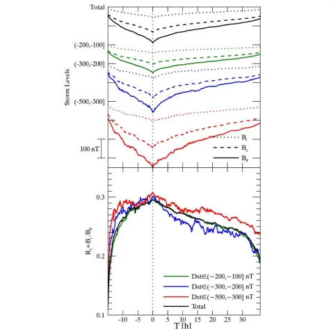
results with equation (3) over HON, KAK, and SJG sta-tions cannot be literally referred to as the Dst index, adopted the same terms for magnetic fields and the ratios just as that used in each station. Figure 6 presents these results, with magnetic components for different storm levels from G1 to G3; the total storms and related ratios are illustrated in the upper and lower panels, respectively.
In Figure 6, the green, blue, and red lines represent G1, G2, and G3, respectively, and black lines represent the av-eraged value of all selected storms. It is obvious that the
internal ratio for the category of total storms, which is represented by the black curve in lower panel, was nearly equal to that of G1. This occurred because the number of events in the G1 category was significantly larger than that in G2 and G3, as shown in Table 1, and naturally carried substantially larger weight in the SEA process.
According to the traces of Ri separately plotted in the
lower panel of Figure 6, it is obvious that for all storm cat-egories, the internal ratios all logarithmically grow to the top values during the main phase. Moreover, significant
local growths, still in the logarithmic manner, are superim-posed on theRitraces for larger storm categories G2 and
G3 corresponding to the multiple temporary intensifica-tion of the magnetic ring current during the main phase. Consequently, the logarithmic form of the local growth of the internal induced fields actually amplifies these tempor-ary intensifications on surface magnetic observations. Re-ferred to as multistep storms or multiple-dip storms, they obviously appear on the curves of the magnetic compo-nents of G2 and G3 in Figure 6 and Figures 1, 2, and 3. The amplification effect to ground magnetic observations is helpful for researchers to more easily identify temporary ring current intensification. Apparently, the corresponding logarithmic growth of the internal induced field to the ex-ternal field also amplifies the entire storm main phase on ground observations.
At the point of the Dst-minimum, the internal ratios showed a small increase from the G1 category, with ratio values of 0.295 ± 0.014, to G2 and G3 categories, holding values of 0.300 ± 0.016 and 0.308 ± 0.015, respectively, as represented in the lower panel of Figure 6. This growth is actually legitimate in physics. Since it is based on Faraday’s law of induction,∇E¼−∂∂Bt, the induction of the mag-netic field from the internal induced current is linearly re-lated to the partial derivative of the external source field with respect to time rather than to the intensity of the ex-ternal source field. For the storms with theDst-minimum less than−200 nT, corresponding to storms in G2 and G3 categories in this study, stronger storms possess shorter main-phase durations on average (Hutchinson et al. 2011) and consequently larger values of the partial derivative of the external source field with respect to time. Therefore, the internal induced magnetic fields on average have lar-ger contributions to surface observations for larlar-ger storms, even if the increase of the contribution ratio of the internal field is not dramatic.
Conclusions
In this paper, we have employed the external source and the internal induced field separation based on the spher-ical harmonic expansion of the disturbed magnetic field to evaluate the influence of induced currents within the Earth on the surface magnetic variations. The main ob-jective of this study is to provide an understanding of the response performance of geomagnetic induction with different disturbance strengths of symmetric ring current. Our results show that the internal induced field and the external source field both maintain the same variation trend with the typical Dst storm evolution covering the main and recovery phases. At the point of the Dst-minimum, the ratio of internal induced fields to surface observations increases with the intensification of storms, from 0.295 ± 0.014 to 0.300 ± 0.016 and 0.308 ±
0.015 corresponding to storm intensity levels of G1: (−200nT,−100nT],G2 : (−300nT,−200nT], and G3: (−500 nT, − 300 nT], respectively. During the storm main phase, the development of internal contribution ra-tio mostly follows the pattern of logarithmic growth with the evolution of the storm up to the top value at the
Dst-minimum before slowly decreasing during the long recovery phase. For larger storms in G2 and G3 categor-ies, remarkable small growths are superimposed on the traces of ratio values during the storm main phase. This effect is caused by the sudden intensification of ener-getic particle injections into the magnetic ring current and mostly occurs during the periods of the main phases of intense storms. This logarithmic growth pat-tern of inpat-ternal induced field obviously amplifies the ef-fects of the ring current intensification on the surface geomagnetic observations and is helpful for researchers to identify the ring current intensification pattern more easily from geomagnetic observations.
It is clear that the geomagnetic induction exceeds lin-ear growth with respect to the increases in external source field, which is physically reasonable and coinci-dent with Faraday’s law of induction ∇E¼−∂∂Bt. Since larger storms relate to larger values of the time derivative of the magnetic field under the assumption of lasting the same approximate duration of storm main phases, this growth is actually reasonable for intense storms led by high-speed CMEs. This internal response of the induced field is a compound reaction encompass-ing the influence of the near-surface environment and the response result of electric conductivity in the upper mantle, which affects the penetration depth of external magnetic signals. Nonetheless, it is still obvious that the contribution rate of the induced field to the surface magnetic field variation increases with an increase in disturbance levels in the magnetospheric ring current.
Although the ratio structure at each station generally fol-lows this pattern, differences are noted among stations. On average, the value ofRiat KAK is slightly larger than that
at HON but is significantly larger than that at SJG. The tendency ofRivariation at HER is different with an
unex-pected higher value in the recovery phase than that in the main phase. The discrepancy among stations could be ex-plained by the lateral anisotropy of electrical conductivity in the upper region of the Earth’s mantle, since the diver-gence among KAK, HON, and SJG stations in our results is coincident with the lateral anisotropies in conductivity of the upper mantle reported by Kelbert et al. (2009). More-over, the surface conductivity discrepancy around stations, particularly the effect of high induction in oceans, also con-tributes to theRidifference among the stations.
to quantify magnetospheric disturbance as a response to interplanetary fluctuation. The research on the observed internal contribution is necessary to provide a comprehen-sive understanding of Dst index variation. Due to differ-ences in the internal contribution ratio among stations, the internal induced and external source field separation could be an essential procedure for each geomagnetic ob-servatory when using surface geomagnetic observations to research the distribution of magnetospheric current systems.
Abbreviations
CIR:interplanetary corotating interaction regions; CME: coronal mass ejection; Dst: disturbance storm time; HER: Hermanus; HON: Honolulu; KAK: Kakioka; SEA: superposed epoch analysis; SJG: San Juan;Sq: solar quiet daily variation.
Competing interests
The authors declare that they have no competing interests.
Authors’contributions
DX developed the main framework. All authors conducted the theoretical considerations and read and approved the final manuscript.
Acknowledgements
We thank the INTERMAGNET organization for supplying the magnetometer data. This work is supported by The Basic Research and Operational Fund of China Earthquake Administration (DQJB12B25) and the National Science Foundation of China, grant no. 41274079.
Received: 26 July 2014 Accepted: 15 January 2015
References
Backus G, Parker R, Constable C (1996) Foundations of geomagnetism. Cambridge Univ, Press, New York
Banks RJ (1969) Geomagnetic variations and the electrical conductivity of the upper mantle. Geophys J Roy Astr S 17:457–487, doi:10.1111/j.1365-246X.1969.tb00252.x
Constable S (1993) Constraints on mantle electrical conductivity from field and laboratory measurements. J Geomagn Geoelectr 45(9):7070–7728 Constable S, Constable C (2004) Observing geomagnetic induction in magnetic
satellite measurements and associated implications for mantle conductivity. Geochem Geophys Geosyst 5, Q01006, doi:10.1029/2003GC000634 Gonzalez W, Joselyn J, Kamide Y, Kroehl H, Rostoker G, Tsurutani B, Vasyliunas V.
(1994) What is a geomagnetic storm? J. Geophys. Res.–Space, (1978–2012). doi:10.1029/93JA02867
Gonzalez W, Tsurutani B, Gonzalez A (1999) Interplanetary origin of geomagnetic storms. Space Sci. Rev. doi:10.1023/A:1005160129098
Gonzalez W, Echer E, Tsurutani B, Gonzalez A, Dal Lago A. (2011) Interplanetary origin of intense, superintense and extreme geomagnetic storms. Space Sci. Rev. doi:10.1007/s11214-010-9715-2
Häkkinen LVT, Pulkkinen TI, Nevanlinna H, Pirjola RJ, Tanskanen EI. (2002) Effects of induced currents on Dst and on magnetic variations at midlatitude stations, J. Geophys. Res. 107(A1), doi:10.1029/2001JA900130
Hamilton D, Gloeckler G, Ipavich F, Stüdemann W, Wilken B, Kremser G (1988) Ring current development during the great geomagnetic storm of February 1986. J Geophys Res 93:14343–14355, doi:10.1029/JA093iA12p14343 Hutchinson J, Wright D, Milan S (2011) Geomagnetic storms over the last solar
cycle: a superposed epoch analysis. J. Geophys. Res., doi:10.1029/ 2011JA016463
Jackson J (1998) Classical electrodynamics. Wiley, New York Kelbert A, Schultz A, Egbert G (2009) Global electromagnetic induction
constraints on transition-zone water content variations. Nature 460 (7258):1003–1006, doi:10.1038/nature08257
Khan A, Kuvshinov A, Semenov A (2011) On the heterogeneous electrical conductivity structure of the Earth’s mantle with implications for transition zone water content. J Geophys Res 116:B01103, doi: 10.1029/2010JB007458
Kuvshinov A, Olsen N (2006) A global model of mantle conductivity derived from 5 years of CHAMP, Ørsted, and SAC-C magnetic data. Geophys Res Lett 33:L18301, doi:10.1029/2006GL027083
Liemohn MW, Jazowski M (2008) Ring current simulations of the 90 intense storms during solar cycle 23. J Geophys Res 113:A00A17, doi:10.1029/ 2008JA013466
Lorrain P, Corson D (1970) Electromagnetic fields and waves. WH Freeman, San Francisco
Mareschal M (1986) Modelling of natural sources of magnetospheric origin in the interpretation of regional induction studies: a review. Surv Geophys 8(3):261–300 Martinec Z, McCreadie H (2004) Electromagnetic induction modelling based on
satellite magnetic vector data. Geophys J Int 157:10451060, doi:10.1111/ j.1365-246X.2004.02252.x
Olsen N (1999) Long-period (30 days–1 year) electromagnetic sounding and the electrical conductivity of the lower mantle beneath Europe. Geophys J Int 138:179–187, doi:10.1046/j.1365-246x.1999.00854.x
Price AT (1967) Electromagnetic induction within the Earth. In: Matsushita S, Campbell WH (eds) Physics of Geomagnetic Phenomena, vol. I. Academic, San Diego, Calif, p 235
Püthe P (2013a) Determination of the 1-D distribution of electrical conductivity in Earth’s mantle from Swarm satellite data. Earth Planets Space 65:12331237, doi:10.5047/eps.2013.07.007
Püthe P (2013b) Determination of the 3-D distribution of electrical conductivity in Earth’s mantle from Swarm satellite data: frequency domain approach based on inversion of induced coefficients. Earth Planets Space 65:12471256, doi:10.5047/eps.2013.09.004
Sabaka TJ, Hulot G, Olsen N (2010) Mathematical properties relevant to geomagnetic field modelling. In: Freeden W, Nashed Z, Sonar T (eds) Handbook of Geomathematics. Springer, Heidelberg
Schultz A, Larsen JC (1990) On the electrical conductivity of Earth’s interior: II. Delineation of heterogeneity by application of extremal inverse solution. Geophys J Int 101:565–590
Sugiura M (1964) Hourly values of the equatorial Dst for the IGY, Ann. IGY 35:9–45 Sugiura M, Kamei T (1991) Equatorial Dst Index: 1957–1986. In: Berthelier A, Menvielle
M (eds) IAGA Bull., vol. 40. ISGI Publ. Off., Saint-Maur-des-Fosses, France Temerin M, Li X (2002) A new model for the prediction of Dst on the basis of the
solar wind. J Geophys Res 107(A12):1472, doi:10.1029/2001JA007532 Temerin M, Li X (2006) Dst model for 1995–2002. J. Geophys. Res., doi:10.1029/
2005JA011257.
Turner N, Baker D, Pulkkinen T, Roeder J, Fennell J, Jordanova V (2001) Energy content in the storm time ring current. J Geophys Res 106:19149–19156, doi:10.1029/2000JA003025
Velímský V (2013) Determination of three-dimensional distribution of electrical conductivity in the Earth’s mantle from Swarm satellite data: time-domain approach. Earth Planets Space 65:12391246, doi:10.5047/eps.2013.08.001 Xu D, Chen T, Zhang X, Liu Z (2009) Statistical relationship between solar wind
conditions and geomagnetic storms in 1998–2008. Planet. Space Sci. doi:10.1016/j.pss.2009.07.015
Submit your manuscript to a
journal and benefi t from:
7Convenient online submission 7Rigorous peer review
7Immediate publication on acceptance 7Open access: articles freely available online 7High visibility within the fi eld
7Retaining the copyright to your article