Volume 2007, Article ID 19070,19pages doi:10.1155/2007/19070
Research Article
Survey of Channel and Radio Propagation Models for
Wireless MIMO Systems
P. Almers,1E. Bonek,2A. Burr,3N. Czink,2, 4M. Debbah,5V. Degli-Esposti,6H. Hofstetter,5P. Ky ¨osti,7 D. Laurenson,8G. Matz,2A. F. Molisch,9, 1C. Oestges,10and H. ¨Ozcelik2
1Department of Electroscience, Lund University, P.O. Box 118, 221 00 Lund, Sweden
2Institut f¨ur Nachrichtentechnik und Hochfrequenztechnik, Technische Universit¨at Wien, Gußhausstraße, 1040 Wien, Austria 3Department of Electronics, University of York, Heslington, York YO10 5DD, UK
4Forschungszentrum Telekommunikation Wien (ftw.), Donau City Straße 1, 1220 Wien, Austria
5Mobile Communications Group, Institut Eurecom, 2229 Route des Cretes, BP193, 06904 Sophia Antipolis, France 6Dipartimento di Elettronica, Informatica e Sistemistica, Universit`a di Bologna, Villa Griffone, 40044 Pontecchio Marconi,
Bologna, Italy
7Elektrobit, Tutkijantie 7, 90570 Oulu, Finland
8Institute for Digital Communications, School of Engineering and Electronics, The University of Edinburgh, Mayfield Road, Edinburgh EH9 3JL, UK
9Mitsubishi Electric Research Lab, 558 Central Avenue, Murray Hill, NJ 07974, USA 10Microwave Laboratory, Universite catholique de Louvain, 1348 Louvain-la-Neuve, Belgium
Received 24 May 2006; Revised 15 November 2006; Accepted 15 November 2006
Recommended by Rodney A. Kennedy
This paper provides an overview of the state-of-the-art radio propagation and channel models for wireless multiple-input multiple-output (MIMO) systems. We distinguish betweenphysical modelsandanalytical modelsand discuss popular examples from both model types. Physical models focus on the double-directional propagation mechanisms between the location of trans-mitter and receiver without taking the antenna configuration into account. Analytical models capture physical wave propagation and antenna configuration simultaneously by describing the impulse response (equivalently, the transfer function) between the antenna arrays at both link ends. We also review some MIMO models that are included in current standardization activities for the purpose of reproducible and comparable MIMO system evaluations. Finally, we describe a couple of key features of channels and radio propagation which are not sufficiently included in current MIMO models.
Copyright © 2007 P. Almers et al. This is an open access article distributed under the Creative Commons Attribution License, which permits unrestricted use, distribution, and reproduction in any medium, provided the original work is properly cited.
1. INTRODUCTION AND OVERVIEW
Within roughly ten years, multiple-input multiple-output (MIMO) technology has made its way from purely theo-retical performance analyses that promised enormous ca-pacity gains [1,2] to actual products for the wireless mar-ket (e.g., [3–6]). However, numerous MIMO techniques still have not been sufficiently tested under realistic propagation conditions and hence their integration into real applications can be considered to be still in its infancy. This fact under-lines the importance of physically meaningful yet easy-to-use methods to understand and mimic the wireless chan-nel and the underlying radio propagation [7]. Hence, the modeling of MIMO radio channels has attracted much at-tention.
Initially, the most commonly used MIMO model was a spatially i.i.d. flat-fading channel. This corresponds to a so-called “rich scattering” narrowband scenario. It was soon re-alized, however, that many propagation environments result in spatial correlation. At the same time, interest in wideband systems made it necessary to incorporate frequency selec-tivity. Since then, more and more sophisticated models for MIMO channels and propagation have been proposed.
1.1. Notation
We briefly summarize the notation used throughout the pa-per. We use boldface characters for matrices (upper case) and vectors (lower case). Superscripts (·)T, (·)H, and (·)∗denote
transposition, Hermitian transposition, and complex conju-gation, respectively. Expectation (ensemble averaging) is de-notedE{·}. The trace, determinant, and Frobenius norm of a matrix are written as tr{·}, det{·}, and · F, respectively. The Kronecker product, Schur-Hadamard product, and vec-torization operation are denoted⊗,, and vec{·}, respec-tively. Finally,δ(·) is the Dirac delta function andInis the n×nidentity matrix.
1.2. Previous work
An introduction to wireless communications and channel modeling is offered in [8]. The book gives a good overview about propagation processes, and large- and small-scale ef-fects, but without touching multiantenna modeling.
A comprehensive introduction to wireless channel mod-eling is provided in [7]. Propagation phenomena, the statis-tical description of the wireless channel, as well as directional MIMO channel characterization and modeling concepts are presented.
Another general introduction to space-time communi-cations and channels can be found in [9], though the book concentrates more on MIMO transmitter and receiver algo-rithms.
A very detailed overview on propagation modeling with focus on MIMO channel modeling is presented in [10]. The authors give an exclusive summary of concepts, mod-els, measurements, parameterization and validation results from research conducted within the COST 273 framework [11].
1.3. MIMO system model
In this section, we first discuss the characterization of wire-less channels from a propagation point of view in terms of the double-directional impulse response. Then, the system level perspective of MIMO channels is discussed. We will show how these two approaches can be brought together. Later in the paper we will distinguish between “physical” and “ana-lytical” models for characterization purposes.
1.3.1. Double-directional radio propagation
In wireless communications, the mechanisms of radio prop-agation are subsumed into the impulse response of the chan-nel between the positionrTxof the transmitter (Tx) and the position rRx of the receiver (Rx). With the assumption of ideal omnidirectional antennas, the impulse response con-sists of contributions of all individual multipath compo-nents (MPCs). Disregarding polarization for the moment, the temporal and angular dispersion effects of a static (time-invariant) channel are described by the double-directional
channel impulse response [12–15] departure (DoD), and the direction of arrival (DoA), respec-tively.1Furthermore,Lis the total number of MPCs
(typi-cally those above the noise level of the system considered). For planar waves, the contribution of thelth MPC, denoted hl(rTx,rRx,τ,φ,ψ), equals DoD, and DoA, respectively, associated with the lth MPC. Nonplanar waves can be modeled by replacing the Dirac deltas in (2) with other appropriately chosen functions2(e.g.,
see [16]).
Fortime-variant(nonstatic) channels, the MPC parame-ters in (2) (al,τl,φl,ψl) the Tx and Rx position (rTx,rRx), and the number of MPCs (L) may become functions of timet. We then replace (1) by the more generaltime-variant double-directional channel impulse response
Polarization can be taken into account by extending the impulse response to a polarimetric (2×2) matrix [17] that describes the coupling between vertical (V) and horizontal (H) polarizations3:
We note that even for single antenna systems, dual-polariza-tion results in a 2×2 MIMO system. In terms of plane wave MPCs, we have
1DoA and DoD are to be understood as spatial angles that correspond to a
point on the unit sphere and replace the spherical azimuth and elevation angles.
2Since Maxwell’s equations are linear, nonplanar waves can alternatively be
broken down into a linear superposition of (infinite) plane waves. How-ever, because of receiver noise it is sufficient to characterize the channel by a finite number of waves.
3The V and H polarization are sufficient for the characterization of the far
Tx Rx
Figure1: Schematic illustration of a MIMO system with multiple transmit and receive antennas.
Here, the “complex amplitude” is itself a polarimetric ma-trix that accounts for scatterer4 reflectivity and
depolariza-tion. We emphasize that the double-directional impulse re-sponse describes only the propagation channel and is thus completely independent of antenna type and configuration, system bandwidth, or pulse shaping.
1.3.2. MIMO channel
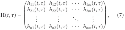
In contrast to conventional communication systems with one transmit and one receive antenna, MIMO systems are equipped with multiple antennas at both link ends (see Figure 1). As a consequence, the MIMO channel has to be described for all transmit and receive antenna pairs. Let us consider ann×mMIMO system, where mandnare the number of transmit and receive antennas, respectively. From a system level perspective, a linear time-variant MIMO chan-nel is then represented by ann×mchannel matrix
H(t,τ)=
where hi j(t,τ) denotes the time-variant impulse response between the jth transmit antenna and the ith receive an-tenna. There is no distinction between (spatially) separate antennas and different polarizations of the same antenna. If polarization-diverse antennas are used, each element of the
4Throughout this paper, the term scatterer refers to any physical object
in-teracting with the electromagnetic field in the sense of causing reflection, diffraction, attenuation, and so forth. The more precise term “interacting objects” has been used in [17,18].
matrixH(t,τ) has to be replaced by a polarimetric subma-trix, effectively increasing the total number of antennas used in the system.
The channel matrix (7) includes the effects of an-tennas (type, configuration, etc.) and frequency filtering (bandwidth-dependent). It can be used to formulate an over-all MIMO input-output relation between the length-m trans-mit signal vectors(t) and the length-nreceive signal vector
y(t) as
y(t)=
τH(t,τ)s(t−τ)dτ+n(t). (8) (Here,n(t) models noise and interference.)
If the channel is time-invariant, the dependence of the channel matrix ontvanishes (we writeH(τ) =H(t,τ)). If the channel furthermore is frequency flat there is just one single tap, which we denote byH. In this case (8) simplifies to
y(t)=Hs(t) +n(t). (9)
1.3.3. Relationship
We have just seen two different views of the radio channel: on the one hand the double-directional impulse response that characterizes the physical propagation channel, on the other hand the MIMO channel matrix that describes the channel on a system level including antenna properties and pulse shaping. We next provide a link between these two approaches, disregarding polarization for simplicity. To this end, we need to incorporate the antenna pattern and pulse shaping into the double-directional impulse response. It can then be shown that
ith receive antenna, respectively. Furthermore, G(Txi)(φ) and
G(Rxj)(ψ) represent the transmit and receive antenna patterns,
respectively, and f(τ) is the overall impulse response of Tx and Rx antennas and frequency filters.
To determine all entries of the channel matrixH(t,τ) via (10), the double-directional impulse response in general must be available for all combinations of transmit and receive antennas. However, under the assumption of planar waves and narrowband arrays this requirement can be significantly relaxed (see, e.g., [19]).
1.4. Model classification
A variety of MIMO channel models, many of them based on measurements, have been reported in the last years. The pro-posed models can be classified in various ways.
Antenna configuration Bandwidth
Physical wave propagation Physical models:
(i) deterministic: - ray tracing
- stored measurements (ii) geometry-based
stochastic: - GSCM (iii) nongeometrical
stochastic: - Saleh-Valenzuela type - Zwick model
MIMO channel matrix Analytical models:
(i) correlation-based: - i.i.d. model - Kronecker model - Weichselberger model (ii) propagation-motivated: - finite-scatterer model - maximum entropy
model - virtual channel
representation
“Standardized” models:
(i) 3GPP SCM (ii) COST 259 and 273 (iii) IEEE 802.11 n (iv) IEEE 802.16 e / SUI (v) WINNER
Figure2: Classification of MIMO channel and propagation models according to [19, Chapter 3.1].
that is,narrowband(flat fading) versuswideband (frequency-selective) models,time-varying versustime-invariant mod-els, and so forth. Narrowband MIMO channels are com-pletely characterized in terms of their spatial structure. In contrast, wideband (frequency-selectivity) channels require additional modeling of the multipath channel characteris-tics. With time-varying channels, one additionally requires a model for the temporal channel evolution according to cer-tain Doppler characteristics.
Hereafter, we will focus on another particularly useful model classification pertaining to the modeling approach taken. An overview of this classification is shown inFigure 2. The fundamental distinction is betweenphysical modelsand analytical models. Physical channel models characterize an environment on the basis of electromagnetic wave propaga-tion by describing the double-direcpropaga-tional multipath propa-gation [12,17] between the location of the transmit (Tx) array and the location of the receive (Rx) array. They ex-plicitly model wave propagation parameters like the complex amplitude, DoD, DoA, and delay of an MPC. More sophis-ticated models also incorporate polarization and time vari-ation. Depending on the chosen complexity, physical mod-els allow for an accurate reproduction of radio propaga-tion. Physical models are independent of antenna config-urations (antenna pattern, number of antennas, array ge-ometry, polarization, mutual coupling) and system band-width.
Physical MIMO channel models can further be split into deterministic models,geometry-based stochastic models, and nongeometric stochastic models. Deterministic models characterize the physical propagation parameters in a
com-pletely deterministic manner (examples are ray tracing and stored measurement data). With geometry-based stochas-tic channel models (GSCM), the impulse response is char-acterized by the laws of wave propagation applied to spe-cific Tx, Rx, and scatterer geometries, which are chosen in a stochastic (random) manner. In contrast, nongeomet-ric stochastic models describe and determine physical pa-rameters (DoD, DoA, delay, etc.) in a completely stochas-tic way by prescribing underlying probability distribution functions without assuming an underlying geometry (ex-amples are the extensions of the Saleh-Valenzuela model [20,21]).
In contrast to physical models, analytical channel mod-els characterize the impulse response (equivalently, the trans-fer function) of the channel between the individual transmit and receive antennas in a mathematical/analytical way with-out explicitly accounting for wave propagation. The individ-ual impulse responses are subsumed in a (MIMO) channel matrix. Analytical models are very popular for synthesizing MIMO matrices in the context of system and algorithm de-velopment and verification.
For the purpose of comparing different MIMO sys-tems and algorithms, various organizations defined reference MIMO channel models which establish reproducible chan-nel conditions. With physical models this means to spec-ify a channel model, reference environments, and parameter values for these environments. With analytical models, pa-rameter sets representative for the target scenarios need to be prescribed.5Examples for such reference models are the
ones proposed within 3GPP [30], IST-WINNER [31], COST 259 [17,18], COST 273 [11], IEEE 802.16a,e [32], and IEEE 802.11n [33].
1.5. Stationarity aspects
Stationarity refers to the property that the statistics of the channel are time- (and frequency-) independent, which is important in the context of transceiver designs trying to cap-italize on long-term channel properties. Channel stationarity is usually captured via the notion ofwide-sense stationary un-correlated scattering(WSSUS) [34,35]. A dual interpretation of the WSSUS property is in terms of uncorrelated multipath (delay-Doppler) components.
In practice, the WSSUS condition is never satisfied ex-actly. This can be attributed to distance-dependent path loss, shadowing, delay drift, changing propagation scenario, and so forth that cause nonstationary long-term channel fluctu-ations. Furthermore, reflections by the same physical object and delay-Doppler leakage due to band- or time-limitations caused by antennas or filters at the Tx/Rx result in corre-lations between different MPCs. In the MIMO context, the nonstationarity of the spatial channel statistics is of particu-lar interest.
The discrepancy between practical channels and the WS-SUS assumption has been previously studied, for example, in [36]. Experimental evidence of non-WSSUS behavior in-volving correlated scattering has been provided, for example, in [37,38]. Nonstationarity effects and scatterer (tap) cor-relation have also found their ways into channel modeling and simulation: see [18] for channel models incorporating large-scale fluctuations and [39] for vector AR channel mod-els capturing tap correlations. A solid theoretical framework for the characterization of non-WSSUS channels has recently been proposed in [40].
In practice, one usually resorts to some kind of qua-sistationarity assumption, requiring that the channel statis-tics stay approximately constant within a certain stationarity time and stationarity bandwidth [40]. Assumptions of this type have their roots in the QWSSUS model of [34] and are relevant to a large variety of communication schemes. As an example, consider ergodic MIMO capacity which can only be achieved with signalling schemes that average over many independent channel realizations having the same statistics [41]. For a channel with coherence timeTcand stationarity time Ts, independent realizations occur approximately
ev-5Some reference models offer both concepts; they specify the geometric
properties of the scatterers using a physical model, but they also provide an analytical model derived from the physical one for easier implementa-tion, if needed.
eryTcseconds and the channel statistics are approximately constant withinTsseconds. Thus, to be able to achieve er-godic capacity, the ratio Ts/Tc has to be sufficiently large. Similar remarks apply to other communication techniques that try to exploit specific long-term channel properties or whose performance depends on the amount of tap correla-tion (e.g., [42]).
To assess the stationarity time and bandwidth, sev-eral approaches have been proposed in the SISO, SIMO, and MIMO context, mostly based on the rate of varia-tion of certain local channel averages. In the context of SISO channels, [43] presents an approach that is based on MUSIC-type wave number spectra (that correspond to spe-cific DOAs) estimated from subsequent virtual antenna array data. The channel non-stationarity is assessed via the amount of change in the wave number power. In contrast, [13,44] de-fines stationarity intervals based on the change of the power delay profile (PDP). To this end, empirical correlations of consecutive instantaneous PDP estimates were used. Regard-ing SIMO channel nonstationarity, [45] studied the variation of the SIMO channel correlation matrix with particular fo-cus on performance metrics relevant in the SIMO context (e.g., beamforming gain). In a similar way, [46] measures the penalty of using outdated channel statistics for spatial pro-cessing via a so-calledF-eigen ratio, which is particularly rel-evant for transmissions in a low-rank channel subspace.
The nonstationarity of MIMO channels has recently been investigated in [47]. There, the SISO framework of [40] has been extended to the MIMO case. Furthermore, comprehen-sive measurement evaluations were performed based on the normalized inner product
trR1 HR2H
R1
HFRH2F
(11)
of two spatial channel correlation matricesR1
H andR2H that
correspond to different time instants.6
This measure ranges from 0 (for channels with orthog-onal correlation matrices, that is, completely disjoint spatial characteristics) to 1 (for channels whose correlation matri-ces are scalar multiples of each other, that is, with identical spatial structure). Thus, this measure can be used to reli-ably describe the evolution of the long-term spatial channel structure. For the indoor scenarios considered in [47], it was concluded that significant changes of spatial channel statis-tics can occur even at moderate mobility.
2. PHYSICAL MODELS
2.1. Deterministic physical models
Physical propagation models are termed “deterministic” if they aim at reproducing the actual physical radio propa-gation process for a given environment. In urban environ-ments, the geometric and electromagnetic characteristics of
6Of course these correlation matrices have to be estimated over sufficiently
Tx Rx
(a)
Tx
Wall Corner Rx
Corner Wall Wall Rx Wall Wall
Rx
(b)
Figure3: Simple RT illustration: (a) propagation scenario (gray shading indicates buildings); (b) corresponding visibility tree (first three layers shown).
the environment and of the radio link can be easily stored in files (environment databases) and the corresponding prop-agation process can be simulated through computer pro-grams. Buildings are usually represented as polygonal prisms with flat tops, that is, they are composed of flat polygons (walls) and piecewise rectilinear edges. Deterministic models are physically meaningful, and potentially accurate. How-ever, they are only representative for the environment con-sidered. Hence, in many cases, multiple runs using diff er-ent environmer-ents are required. Due to the high accuracy and adherence to the actual propagation process, determin-istic models may be used to replace measurements when time is not sufficient to set up a measurement campaign or when particular cases, which are difficult to measure in the real world, will be studied. Although electromagnetic mod-els such as the method of moments (MoM) or the finite-difference in time domain(FDTD) model may be useful to study near field problems in the vicinity of the Tx or Rx antennas, the most appropriate physical-deterministic mod-els for radio propagation, at least in urban areas, are ray tracing (RT) models. RT models use the theory of geomet-rical optics to treat reflection and transmission on plane surfaces and diffraction on rectilinear edges [48]. Geomet-rical optics is based on the so-called ray approximation, which assumes that the wavelength is sufficiently small com-pared to the dimensions of the obstacles in the environ-ment. This assumption is usually valid in urban radio prop-agation and allows to express the electromagnetic field in terms of a set of rays, each one of them corresponding to a piecewise linear path connecting two terminals. Each “cor-ner” in a path corresponds to an “interaction” with an ob-stacle (e.g., wall reflection, edge diffraction). Rays have a null transverse dimension and therefore can in principle de-scribe the field with infinite resolution. If beams (tubes of flux) with a finite transverse dimension are used instead
of rays, then the resulting model is calledbeam launching, or ray splitting. Beam launching models allow faster field strength prediction but are less accurate in characterizing the radio channel between two SISO or MIMO terminals. Therefore, only RT models will be described in further de-tail here.
2.1.1. Ray-tracing algorithm
With RT algorithms, initially the Tx and Rx positions are specified and then all possible paths (rays) from the Tx to the Rx are determined according to geometric considera-tions and the rules of geometrical optics. Usually, a maxi-mum numberNmaxof successive reflections/diffractions
(of-ten called prediction order) is prescribed. This geometric “ray tracing” core is by far the most critical and time con-suming part of the RT procedure. In general, one adopts a strategy that captures the individual propagation paths via a so-called visibility tree (see Figure 3). The visibility tree consists of nodes and branches and has a layered structure. Each node of the tree represents an object of the scenario (a building wall, a wedge, the Rx antenna, dots) whereas each branch represents a line-of-sight (LoS) connection between two nodes/objects. The root node corresponds to the Tx an-tenna.
The visibility tree is constructed in a recursive manner, starting from the root of the tree (the Tx). The nodes in the first layer correspond to all objects for which there is an LoS to the Tx. In general, two nodes in subsequent layers are con-nected by a branch if there is LoS between the corresponding physical objects. This procedure is repeated until layerNmax
creation of the visibility tree may be highly computationally complex, especially in a full 3D case and ifNmaxis large.
Once the visibility tree is built, a backtracking procedure determines the path of each ray by starting from the corre-sponding leaf, traversing the tree upwards to the root node, and applying the appropriate geometrical optics rules at each traversed node. To theith ray, a complex, vectorial electric field amplitudeEiis associated, which is computed by tak-ing into account the Tx-emitted field, free space path loss, and the reflections, diffractions, and so forth experienced by the ray. Reflections are accounted for by applying the Fresnel reflection coefficients [48], whereas for diffractions the field vector is multiplied by appropriate diffraction coefficients obtained from the uniform geometrical theory of diffraction [49,50]. The distance-decay law (divergence factor) may vary along the way due to diffractions (see [49]). The resulting field vector at the Rx position is composed of the fields for each of theNrrays asERx=
Nr
i=0ERxi with
ERxi =ΓiBiETxi withBi=Ai,NiAi,Ni−1· · ·Ai,1. (12)
Here,Γiis the overall divergence factor for theith path (this depends on the length of all path segments and the type of interaction at each of its nodes),Ai,jis a rank-one matrix that decomposes the field into orthogonal components at the jth node (this includes appropriate attenuation, reflection, and diffraction coefficients and thus depends on the interaction type),Ni ≤ Nmax is the number of interactions (nodes) of
theith path, andETxi is the field at a reference distance of 1 m from the Tx in the direction of theith ray.
2.1.2. Application to MIMO channel characterization
To obtain the mapping of a channel input signal to the nel output signal (and thereby all elements of a MIMO chan-nel matrix H), (12) must be augmented by taking into ac-count the antenna patterns and polarization vectors at the Tx and Rx [51]. Note that this has the advantage that diff er-ent antenna types and configurations can be easily evaluated for the same propagation environment. Moreover, accurate, site-specific MIMO performance evaluation is possible (e.g., [52]).
Since all rays at the Rx are characterized individually in terms of their amplitude, phase, delay, angle of departure, and angle of arrival, RT allows a complete characterization of propagation [53] as far as specular reflections or diffractions are concerned. However, traditional RT methods neglect dif-fuse scattering which can be significant in many propagation environments (diffuse scattering refers to the power scattered in other than the specular directions which is due to non-ideal scatterer surfaces). Since diffuse scattering increases the “viewing angle” at the corresponding node of the visibility tree, it effectively increases the number of rays. This in turn has a noticeable impact on temporal and angular dispersion and hence on MIMO performance. This fact has motivated growing recent interest in introducing some kind of diffuse scattering into RT models. For example, in [54], a simple dif-fuse scattering model has been inserted into a 3D RT method; RT augmented by diffuse scattering was seen to be in better
agreement with measurements than classical RT without dif-fuse scattering.
2.2. Geometry-based stochastic physical models
Any geometry-based model is determined by the scatterer locations. In deterministic geometrical approaches (like RT discussed in the previous subsection), the scatterer locations are prescribed in a database. In contrast, geometry-based stochastic channel models (GSCM) choose the scatterer lo-cations in a stochastic (random) fashion according to a cer-tain probability distribution. The actual channel impulse re-sponse is then found by a simplified RT procedure.
2.2.1. Single-bounce scattering
GSCM were originally devised for channel simulation in sys-tems with multiple antennas at the base station (diversity antennas, smart antennas). The predecessor of the GSCM in [55] placed scatterers in a deterministic way on a cir-cle around the mobile station, and assumed that only sin-gle scattering occurs (i.e., one interacting object between Tx and Rx). Roughly twenty years later, several groups simul-taneously suggested to augment this single-scattering model by using randomly placed scatterers [56–61]. This random placement reflects physical reality much better. The single-scattering assumption makes RT extremely simple: apart from the LoS, all paths consist of two subpaths connecting the scatterer to the Tx and Rx, respectively. These subpaths characterize the DoD, DoA, and propagation time (which in turn determines the overall attenuation, usually according to a power law). The scatterer interaction itself can be taken into account via an additional random phase shift.
A GSCM has a number of important advantages [62]:
(i) it has an immediate relation to physical reality; impor-tant parameters (like scatterer locations) can often be determined via simple geometrical considerations; (ii) many effects are implicitly reproduced: small-scale
fading is created by the superposition of waves from individual scatterers; DoA and delay drifts caused by MS movement are implicitly included;
(iii) all information is inherent to the distribution of the scatterers; therefore, dependencies of power delay pro-file (PDP) and angular power spectrum (APS) do not lead to a complication of the model;
(iv) Tx/Rx and scatterer movement as well as shadowing and the (dis)appearance of propagation paths (e.g., due to blocking by obstacles) can be easily imple-mented; this allows to include long-term channel cor-relations in a straightforward way.
BS NS
MS Far
scatterer cluster
Local scatterers
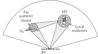
Figure4: Principle of the GSCM (BS—base station, MS—mobile station).
suggests to place the scatterers randomly around the MS [58,60]. In [63], various other scatterer distributions around the MS were analyzed; a one-sided Gaussian distribution with respect to distance from the MS resulted in an approx-imately exponential PDP, which is in good agreement with many measurement results. To make the density or strength of the scatterers depend on distance, two implementations are possible. In the “classical” approach, the probability den-sity function of the scatterers is adjusted such that scatter-ers occur less likely at large distances from the MS. Alter-natively, the “nonuniform scattering cross section” method places scatterers with uniform density in the considered area, but down-weights their contributions with increasing dis-tance from the MS [62]. For very high scatterer density, the two approaches are equivalent. However, nonuniform scat-tering cross-section can have numerical advantages, in par-ticular less statistical fluctuations of the power-delay profile when the number of scatterers is finite.
Another important propagation effect arises from the existence of clusters of far scatterers (e.g., large buildings, mountains, and so forth). Far scatterers lead to increased temporal and angular dispersion and can thus significantly influence the performance of MIMO systems. In a GSCM, they can be accounted for by placing clusters of far scatterers at random locations in the cell [60] (seeFigure 4).
2.2.2. Multiple-bounce scattering
All of the above considerations are based on the assumption that only single-bounce scattering is present. This is restric-tive insofar as the position of a scatterer completely deter-mines DoD, DoA, and delay, that is, only two of these param-eters can be chosen independently. However, many environ-ments (e.g., micro- and picocells) feature multiple-bounce scattering for which DoD, DoA, and delay are completely de-coupled. In microcells, the BS is below rooftop height, so that propagation mostly consists of waveguiding through street canyons [64, 65], which involves multiple reflections and diffractions (this effect can be significant even in macrocells [66]). For picocells, propagation within a single large room is mainly determined by LoS propagation and single-bounce reflections. However, if the Tx and Rx are in different rooms, then the radio waves either propagate through the walls or they leave the Tx room, for example, through a window or
door, are waveguided through a corridor, and be diffracted into the room with the Rx [67].
If the directional channel properties need to be repro-duced only for one link end (i.e., multiple antennas only at the Tx or Rx), multiple-bounce scattering can be incor-porated into a GSCM via the concept ofequivalent scatter-ers. These are virtual single-bounce scatterers whose posi-tions and pathloss are chosen such that they mimic multiple bounce contributions in terms of their delay and DoA (see Figure 5). This is always possible since the delay, azimuth, and elevation of a single-bounce scatterer are in one-to-one correspondence with its Cartesian coordinates. A similar re-lationship exists on the level of statistical characterizations for the joint angle-delay power spectrum and the probability density function of the scatterer coordinates (i.e., the spatial scatterer distribution). For further details, we refer to [17].
In a MIMO system, the equivalent scatterer concept fails since the angular channel characteristics are reproduced cor-rectly only for one link end. As a remedy, [68] suggested the use of double scattering where the coupling between the scat-terers around the BS and those around the MS is established by means of a so-called illumination function (essentially a DoD spectrum relative to that scatterer). We note that the channel model in that paper also features simple mechanisms to include waveguiding and diffraction.
Another approach to incorporate multiple-bounce scat-tering into GSCM models is the twin-cluster concept pur-sued within COST 273 [11]. Here, the BS and MS views of the scatterer positions are different, and a coupling is estab-lished in terms of a stochastic link delay. This concept indeed allows for decoupled DoA, DoD, and delay statistics.
2.3. Nongeometrical stochastic physical models
Nongeometrical stochastic models describe paths from Tx to Rx by statistical parameters only, without reference to the ge-ometry of a physical environment. There are two classes of stochastic nongeometrical models reported in the literature. The first one uses clusters of MPCs and is generally called the extended Saleh-Valenzuela model since it generalizes the temporal cluster model developed in [69]. The second one (known as Zwick model) treats MPCs individually.
2.3.1. Extended Saleh-Valenzuela model
Saleh and Valenzuela proposed to model clusters of MPCs in the delay domain via a doubly exponential decay process [69] (a previously considered approach used a two-state Poisson process [65]). The Saleh-Valenzuela model uses one expo-nentially decaying profile to control the power of a multipath cluster. The MPCs within the individual clusters are then characterized by a second exponential profile with a steeper slope.
BS
MS
Figure5: Example for equivalent scatterer () in the uplink of a system with multiple element BS antenna (true scatterers shown as
).
no contrary evidence was initially available since the model was developed from SIMO measurements.) These assump-tions allow to characterize the spatial clusters in terms of their mean cluster angle and the cluster angular spread (cf. [71]). Usually, the mean cluster angleΘ is assumed to be uniformly distributed within [0, 2π) and the angleϕof the MPCs in the cluster are Laplacian distributed, that is, their probability density function equals
p(ϕ)=√c
2σexp
− √
2 σ |ϕ−Θ|
, (13)
whereσcharacterizes the cluster’s angular spread andcis an appropriate normalization constant [35]. The mean delay for each cluster is characterized by a Poisson process, and the in-dividual delays of the MPCs within the cluster are character-ized by a second Poisson process relative to the mean delay.
2.3.2. Zwick model
In [72] it is argued that for indoor channels clustering and multipath fading do not occur when the sampling rate is suf-ficiently large. Thus, in the Zwick model, MPCs are gener-ated independently (no clustering) and without amplitude fading. However, phase changes of MPCs are incorporated into the model via geometric considerations describing Tx, Rx, and scatterer motion. The geometry of the scenario of course also determines the existence of a specific MPC, which thus appears and disappears as the channel impulse response evolves with time. For nonline of sight (NLoS) MPCs, this ef-fect is modeled using a marked Poisson process. If a line-of-sight (LoS) component will be included, it is simply added in a separate step. This allows to use the same basic procedure for both LoS and NLoS environments.
3. ANALYTICAL MODELS
3.1. Correlation-based analytical models
Various narrowband analytical models are based on a mul-tivariate complex Gaussian distribution [21] of the MIMO
channel coefficients (i.e., Rayleigh or Ricean fading). The channel matrix can be split into a zero-mean stochastic part
Hs and a purely deterministic part Hd according to (e.g., [73])
H=
1 1 +KHs+
K
1 +KHd, (14)
whereK≥0 denotes the Rice factor. The matrixHdaccounts for LoS components and other nonfading contributions. In the following, we focus on the NLoS components character-ized by the Gaussian matrixHs. For simplicity, we thus as-sume K = 0, that is,H = Hs. In its most general form, the zero-mean multivariate complex Gaussian distribution ofh=vec{H}is given by7
f(h)= 1
πnmdetRHexp
−hHR−H1h
. (15)
Thenm×nmmatrix
RH=E
hhH (16)
is known asfull correlation matrix (e.g., [27,28]) and de-scribes the spatial MIMO channel statistics. It contains the correlations of all channel matrix elements. Realizations of MIMO channels with distribution (15) can be obtained by8
H=unvec{h} withh=R1H/2g. (17)
Here,R1H/2denotes an arbitrary matrix square root (i.e., any
matrix satisfyingR1H/2RHH/2 =RH), andgis annm×1 vector
with i.i.d. Gaussian elements with zero mean and unit vari-ance.
Note that direct use of (17) in general requires full speci-fication ofRHwhich involves (nm)2real-valued parameters.
To reduce this large number of parameters, several diff er-ent models were proposed that impose a particular structure on the MIMO correlation matrix. Some of these models will next be briefly reviewed. For further details, we refer to [74].
3.1.1. The i.i.d. model
The simplest analytical MIMO model is the i.i.d. model (sometimes referred to as canonical model). HereRH=ρ2I,
that is, all elements of the MIMO channel matrix H are uncorrelated (and hence statistically independent) and have equal varianceρ2. Physically, this corresponds to a spatially
white MIMO channel which occurs only in rich scatter-ing environments characterized by independent MPCs uni-formly distributed in all directions. The i.i.d. model consists just of a single parameter (the channel powerρ2) and is
of-ten used for theoretical considerations like the information theoretic analysis of MIMO systems [1].
7For ann×mmatrixH=[h
1· · ·hm], the vec{·}operator returns the
length-nmvector vec{H} =[hT
1· · ·hTm]T.
3.1.2. The Kronecker model
The so-called Kronecker model was used in [25–27] for ca-pacity analysis before being proposed by [28] in the frame-work of the European Union SATURN project [75]. It as-sumes that spatial Tx and Rx correlation are separable, which is equivalent to restricting to correlation matrices that can be written as Kronecker product
RH=RTx⊗RRx (18)
with the Tx and Rx correlation matrices
RTx=E
HHH, R
Rx=E
HHH, (19)
respectively. It can be shown that under the above assump-tion, (17) simplifies to theKronecker model
h=RTx⊗RRx1/2g⇐⇒H=R1Rx/2GR1Tx/2 (20)
withG = unvec(g) an i.i.d. unit-variance MIMO channel matrix. The model requires specification of the Tx and Rx correlation matrices, which amounts ton2+m2real
param-eters (instead ofn2m2).
The main restriction of the Kronecker model is that it enforces a separable DoD-DoA spectrum [76], that is, the joint DoD-DoA spectrum is the product of the DoD spec-trum and the DoA specspec-trum. Note that the Kronecker model is not able to reproduce the coupling of a single DoD with a single DoA, which is an elementary feature of MIMO chan-nels with single-bounce scattering.
Nonetheless, the model (20) has been used for the the-oretical analysis of MIMO systems and for MIMO channel simulation yielding experimentally verified results when two or maximum three antennas at each link end were involved. Furthermore, the underlying separability of Tx and Rx in the Kronecker sense allows for independent array optimization at Tx and Rx. These applications and its simplicity have made the Kronecker model quite popular.
3.1.3. The Weichselberger model
The Weichselberger model [29, 74] aims at obviating the restriction of the Kronecker model to separable DoA-DoD spectra that neglects significant parts of the spatial structure of MIMO channels. Its definition is based on the eigenvalue decomposition of the Tx and Rx correlation matrices,
RTx=UTxΛTxUH
Tx, RRx=URxΛRxUHRx.
(21)
Here,UTxandURx are unitary matrices whose columns are the eigenvectors ofRTx andRRx, respectively, andΛTx and ΛRxare diagonal matrices with the corresponding
eigenval-ues. The model itself is given by
H=URx(ΩG)UTTx, (22)
whereGis again ann×mi.i.d. MIMO matrix,denotes the Schur-Hadamard product (elementwise multiplication), and
Tx Rx
. . .
. . . . . .
Figure 6: Example of finite scatterer model with single-bounce scattering (solid line), multiple-bounce scattering (dashed line), and a “split” component (dotted line).
Ωis the elementwise square root of ann×mcoupling matrix Ωwhose (real-valued and nonnegative) elements determine the average power coupling between the Tx and Rx eigen-modes. This coupling matrix allows forjointmodeling of the Tx and Rx channel correlations. We note that the Kronecker model is a special case of the Weichselberger model obtained with therank-one coupling matrixΩ = λRxλTTx, whereλTx
andλRxare vectors containing the eigenvalues of the Tx and
Rx correlation matrix, respectively.
The Weichselberger model requires specification of the Tx and Rx eigenmodes (UTx andURx) and of the coupling
matrixΩ. In general, this amounts ton(n−1)+m(m−1)+nm real parameters. These are directly obtainable from measure-ments. We emphasize, however, that capacity (mutual infor-mation) and diversity order of a MIMO channel are inde-pendent of the Tx and Rx eigenmodes; hence, their analy-sis requires only the coupling matrixΩ(nmparameters). In particular, the structure ofΩdetermines which MIMO gains (diversity, capacity, or beamforming gain) can be exploited which helps to design signal-processing algorithms. Some in-structive examples are discussed in [74, Chapter 6.4.3.4].
3.2. Propagation-motivated analytical models
3.2.1. Finite scatterer model
The fundamental assumption of the finite scatterer model is that propagation can be modeled in terms of a finite number P of multipath components (cf.Figure 6). For each of the components (indexed by p), a DoDφp, DoA ψp, complex amplitudeξp, and delayτpis specified.9
The model allows for single-bounce and multiple-bounce scattering, which is in contrast to GSCMs that usually only incorporate single-bounce and double-bounce scatter-ing. The finite scatterer models even allow for “split” com-ponents (seeFigure 6), which have a single DoD but subse-quently split into two or more paths with different DoAs (or vice versa). The split components can be treated as multiple components having the same DoD (or DoA). For more de-tails we refer to [22,77].
9For simplicity, we restrict to the 2D case where DoA and DoD are
Given the parameters of all MPCs, the MIMO channel matrixHfor the narrowband case (i.e., neglecting the delays τp) is given by
H=
P
p=1
ξpψψp
φTφ p
=ΨΞΦT, (23)
where Φ = [φ(φ1)· · ·φ(φP)], Ψ = [ψ(ψ1)· · ·ψ(ψP)], φT(φ
p) andψ(ψp) are the Tx and Rx steering vectors cor-responding to thepth MPC, andΞ=diag(ξ1,. . .,ξP) is a di-agonal matrix consisting of the multipath amplitudes. Note that the steering vectors incorporate the geometry, directiv-ity, and coupling of the antenna array elements. For wide-band systems, also the delays must be taken into account. Including the bandlimitation to the system bandwidthB =
1/Tsinto the channel, the resulting tapped delay line repre-sentation of the channel readsH(τ)= ∞l=−∞Hlδ(τ −lTs) with
Hl= P
p=1
ξpsinc
τp−lTs
ψψp
φTφ p
=ΨΞTl
ΦT,
(24)
where sinc(x) = sin(πx)/(πx) andTl is a diagonal matrix with diagonal elements sinc(τp−lTs), p=1,. . .,P. Further details can be found in [78].
The finite scatterer model can be interpreted as a straight-forward way to calculate (10) (seeSection 1.3.3). It is com-patible with many other models (e.g., the 3GPP model [30]) that define statistical distributions for the MPC parameters. Other environment dependent distributions of these param-eters may be inferred from measurements. For example, the measurements in [78] suggest that in an urban environment all multipath parameters are statistically independent and the DoAsψpand DoDsφpare approximately uniformly dis-tributed, the complex amplitudesξphave a log-normally dis-tributed magnitude and uniform phase, and the delaysτpare exponentially distributed.
3.2.2. Maximum entropy model
In [23], the question of MIMO channel modeling based on statistical inference was addressed. In particular, the maxi-mum entropy principle was proposed to determine the dis-tribution of the MIMO channel matrix based on a priori in-formation that is available. This a priori inin-formation might include properties of the propagation environment and sys-tem parameters (e.g., bandwidth, DoAs, etc.). The maximum entropy principle was justified by the objective to avoid any model assumptions not supported by the prior information. As far as consistency is concerned, [23] shows that the target application for which the model has to be consistent can in-fluence the proper choice of the model. Hence, one may ob-tain different channels models for capacity calculations than for bit-error-rate simulations. Since this is obviously unde-sirable, it was proposed to ignore information about any tar-get application when constructing practically useful models. Consistency is then enforced by the following axiom.
Axiom
If the prior information I1 which is the basis for channel
modelH1is equivalent to the prior informationI2of
chan-nel modelH2, then both models must be assigned the same
probability distribution, f(H1)= f(H2).
As an example, consider that the following prior infor-mation is available:
(i) the numberssTxandsRxof scatterers at the Tx and Rx
side, respectively;
(ii) the steering vectors for all Tx and Rx scatterers, con-tained in them×sTxandn×sRx matricesΦandΨ,
respectively;
(iii) the corresponding scatterer powersPTxandPRx; and (iv) the path gains between Tx and Rx scatterers,
charac-terized bysRx×sTxpattern mask (coupling matrix)Ω.
Then, the maximum entropy channel model was shown to equal
H=ΨP1Rx/2(ΩG)P1Tx/2ΦT, (25)
whereGis ansRx×sTxGaussian matrix with i.i.d. elements.
We note that this model is consistent in the sense that less detailed models (for which parts of the prior information are not available) can be obtained by “marginalizing” (25) with respect to the unknown parameters.10Examples include
the i.i.d. Gaussian model where only the channel energy is known (obtained withΦ = Fm whereFm is the length-m DFT matrix,Ψ=Fn,PTx=I, andPRx=I), the DoA model where steering vectors and powers are known only for the Rx side (obtained with Φ = Fm,PTx = I), and the DoD model where steering vectors and powers are known only for the Tx side (obtained withΨ=Fn,PRx =I). We conclude that a useful feature of the maximum entropy approach is the simplicity of translating an increase or decrease of (physical) prior information into the channel distribution model in a consistent fashion.
3.2.3. Virtual channel representation
In [24], a MIMO model called virtual channel representation was proposed as follows:
H=Fn(ΩG)FHm. (26)
Here, the DFT matricesFmandFncontain the steering vec-tors formvirtual Tx andnvirtual Rx scatterers,Gis ann×m i.i.d. zero-mean Gaussian matrix, and Ωis an n×m ma-trix whose elements characterize the coupling of each pair of virtual scatterers, that is, (ΩG) represents the “inner” propagation environment between virtual Tx and Rx scatter-ers. In essence, (26) corresponds to a spatial sampling that collapses all physical DoAs and DoDs into fixed directions
10Models that do not have this property can be shown to contradict Bayes’
determined by the spatial resolution of the arrays. We note that the virtual channel model can be viewed as a special case of the Weichselberger model with Tx and Rx eigenmodes equal to the columns of the DFT matrices. In the case where [Ω]i j = 1, the virtual channel model reduces to the i.i.d. channel model, that is, rich scattering with full connection of (virtual) Tx and Rx scatterer clusters. Due to its simplic-ity, the virtual channel model is mostly useful for theoretical considerations like analyzing the capacity scaling behavior of MIMO channels [79]. It was also shown to be capacity com-plying in [80,81]. However, one has to keep in mind that the virtual representation in terms of DFT steering matri-ces is appropriate only for uniform linear arrays at Tx and Rx.
4. STANDARDIZED MODELS
Standardized models are an important tool for the develop-ment of new radio systems. They allow to assess the benefits of different techniques (signal processing, multiple access, etc.) for enhancing capacity and improving performance, in a manner that is unified and agreed on by many parties. For example, the COST 207 wideband power delay profile model was widely used in the development of GSM, and used as a basis for the decision on modulation and multiple-access methods. In this section, we discuss five standardized direc-tional MIMO channel models to provide an overview of re-cent and ongoing channel modeling activities.
4.1. COST 259/273
“COST” is an abbreviation for European cooperation in the field of scientific and technical research. Several COST initia-tives were dedicated to wireless communications, in partic-ular COST 259 “Flexible personalized wireless communica-tions” (1996–2000) and COST 273 “Towards mobile broad-band multimedia networks” (2001–2005). These initiatives developed channel models that include directional charac-teristics of radio propagation and are thus suitable for the simulation of smart antennas and MIMO systems. They are, at this time, the most general standardized channel models, and are not intended for specific systems. The 3GPP/3GPP2 model and the 802.11n model can be viewed as subsets (though with different parameter settings).
4.1.1. COST 259 directional channel model
The COST 259 directional channel model (DCM) [17,18] is a physical model that gives a model for the delay and an-gle dispersion at BS and MS, for different radio environ-ments. It was the first model that explicitly took the rather complex relationships between BS-MS-distance, delay dis-persion, angular spread, and other parameters into account. It is also general in the sense that it is defined for a 13 different radio environments (e.g., typical urban, bad ur-ban, open square, indoor office, indoor corridor) that in-clude macrocellular, microcellular, and picocellular
scenar-ios.11The modeling approaches for macro-, micro-, and
pic-ocells are different; in the following, we describe only the macrocell approach.
Each radio environment is described byexternal param-eters (e.g., BS position, radio frequency, average BS and MS height) and byglobalparameters, which are sets of probabil-ity densprobabil-ity functions and/or statistical moments character-izing a specific environment (e.g., the number of scatterers is characterized by a Poisson distribution). The determina-tion of the global parameters is partly geometric, and partly stochastic. We place the MS at random in the cell. Similarly, a number of scatterer clusters (see Section 2.2.1) are geo-metrically placed in the cell. From those positions, we can determine the relative delay and mean angles of the diff er-ent clusters that make up the double-directional impulse re-sponse. The angular spread, delay spread, and shadowing, on the other hand, are determined stochastically. They are modeled as correlated lognormally distributed random vari-ables.
Eachradio environment contains a number of propaga-tion environments, which are defined as an area over which the local parameters (which are defined as realizations of the global parameters) are approximately constant; they are typically several meters in diameter. These local parameters are randomly generated realizations of the global parameters and describe the instantaneous channel behavior. As ultimate output of the channel model, the double-directional impulse response is then obtained according to (1)-(2), which then al-lows to derive the transfer function matrix according to (10). The impulse responses can also be generated via a GSCM approach, as described inSection 2.2. It is noteworthy that the COST 259 model can handle the continuous movement of the MS over several propagation environments, and even across different radio environments; details can be found in [17,18].
While fairly general, there are two major restrictions of the COST 259 DCM. On the one hand, scatterers are as-sumedstationaryso that channel time variations are solely due to MS movement; this obviously excludes certain en-vironments (e.g., indoor scenarios with persons moving around). On the other hand, delay attenuations are modeled as complex Gaussian random variables. This requires a suffi -ciently large number of MPCs within each delay bin, a condi-tion that is not met in some situacondi-tions; this latter assumpcondi-tion is also made in all other standardized channel models.
4.1.2. COST 273
The COST 273 channel model [82] shows considerable sim-ilarity to the COST 259 model, but differs in several key re-spects.
11Macrocellshave outdoor BSs above rooftop and either outdoor MSs at
(1) A number of new radio environments is defined, re-flecting the new applications for MIMO systems (e.g., peer-to-peer and fixed-wireless-access scenarios).
(2) The chosen parameters have been updated, based on new available measurement campaigns.
(3) The same modeling approach is used for macro-, micro-, and pico-cells. The approach is similar to the COST 259 approach for macrocells.
(4) The modeling of the distribution of DOAs and DODs is different, compared to the COST 259 model. One cluster is split up into two representations of itself: one that represents the cluster as seen by the BS and one as it is seen by the mobile terminal (MT). Both realizations look identical, like twins. Each ray propagated at the transmitter is bounced at each scatterer in the corresponding cluster and reradiated at the same scatterer of the twin cluster towards the receiver. The two cluster representations are linked via astochastic cluster link delay, which is the same for all scatterers inside a clus-ter. The cluster link delay ensures realistic path delays as, for example, derived from measurement campaigns, whereas the placement of the cluster is driven by the angular statistics of the cluster as observed from BS/MT, respectively.
4.2. 3GPP SCM
The spatial channel model (SCM) [30] was developed by 3GPP/3GPP2 to be a common reference for evaluating dif-ferent MIMO concepts in outdoor environments at a center frequency of 2 GHz and a system bandwidth of 5 MHz.
The SCM consists of two parts: (i) a calibration model, and (ii) a system-simulation model.
4.2.1. Calibration model
The calibration model is an over-simplified channel model whose purpose is to check the correctness of simulation implementations. In the course of standardization work, it is often necessary to compare the implementations of the same algorithm by different companies. Comparing the per-formance of the algorithm in the “calibration” channels al-lows to easily assess whether two implementations are equiv-alent. We stress that the calibration model isnotintended for performance assessment of algorithms or systems.
The calibration model, as described in the 3GPP/3GPP2 standard, can be implemented either as a physical model or as an analytical model. The physical model is a non-geometrical stochastic physical model (compareSection 2.3). It is a spatial extension of the ITU-R channel models [83], which describe the wideband characteristics of the channel as a tapped delay line. Taps with different delays are inde-pendently fading, and each tap is characterized by its own power azimuth spectrum (which is uniform or Laplacian), angular spread (AS), and mean direction, at both the MS and the BS. The parameters (i.e., angular spread, mean di-rection, etc.), are fixed; thus the model represents stationary channel conditions. The Doppler spectrum is defined im-plicitly by introducing speed and direction of travel of the MS.
The model also defines a number of antenna config-urations. Given those, the physical model can be trans-formed into an equivalent analytical model as discussed in Section 3.2.1.
4.2.2. Simulation model
The SCM intended for performance evaluation is called the simulation model.12 The model is a physical model and
distinguishes between three different environments: urban macrocell, suburban macrocell, and urban microcell. The model structure and simulation methodology are identical for all these environments, but the parameters, like angular spread, delay spread, and so forth, are different.
The simulation model employs both geometrical and stochastic components. Let us first describe the simulation procedure for a single link between one MS and one BS. The geometrical component is that the MSs are placed at random within a given cell, and the orientation of the antenna array, as well as the direction of movement within the cell, are also chosen at random. From the MS position, we can determine the bulk pathloss, which is given by the COST 231—Hata model for macrocells, and the COST 231—Walfish-Ikegami model for microcells. The number of taps with different de-lays is 6 (as in the ITU-R models), but their delay and aver-age power are chosen stochastically from a probability den-sity function.
Each tap shows angular dispersion at the BS and the MS; this dispersion is implemented by representing each tap by a number of subpaths that all have the same delay, but diff er-ent DOAs (and DODs). Physically, this means that each path consists of a cluster of 20 scatterers with slightly different di-rections but equal time of arrival. Specifically, the modeling of the angular dispersion works as follows: the mean DOA and DOD of the total arriving power (weighted average over all the taps) is determined by the location of the MS and the orientation of the antenna array. The mean DOA (or DOD) of one tap is chosen at random from a Gaussian distribution that is centered around this total mean (the variance of this distribution is one of the model parameters). The 20 sub-paths have different offsetsΔφifrom this tap mean; those off -sets are fixed and tabulated in the 3GPP standard. Adding up the different subpaths (which all have deterministic ampli-tudes, but different phases) results in Rayleigh or Rice fading. Temporal variations of the impulse response are effected by movement of the MS, which in turn leads to different phase shifts of the subpaths.
When using the SCM, the simulation of the system be-havior is carried out as a sequence of “drops,” where a “drop” is defined as one simulation run over a certain (short) time period. That period is assumed to be short, so that it is jus-tified to assume (as the model does) that large-scale channel parameters, such as angle spread, mean DOA, delay spread, and shadowing stay constant during a drop. For each drop, these large-scale channel parameters are drawn according to
12This name, which is historically motivated, is slightly misleading, as the
distributions functions. The MS positions are varied at ran-dom at the beginning of each drop.
In some cases, we wish to emulate the channels between multiple BScells/sectors andmultiple MSslinked to these BSs. The cell layout and BS locations are fixed for a certain num-ber of successive drops, but (as in the single-cell case) the MS positions are varied at random at the beginning of each drop. Antenna radiation patterns, antenna geometries, and ori-entations can be chosen arbitrary, that is, the model is an-tenna independent. When all the parameters and anan-tenna effects are defined, analytical formulations can be extracted from the physical model. Note that each drop results in a dif-ferent correlation matrix for the analytical model.
In addition to the characteristics described above, the simulation model has several optional features: (i) a polariza-tion model, (ii) far scatterer clusters, (iii) a LoS component for the microcellular case, and (iv) a modified distribution of the angular distribution at the MS, which emulates propaga-tion in an urban street canyon.
4.3. WINNER channel models
The channel models developed in the IST-WINNER [31] project are related to both the COST 259 model (see Section 4.1.1) and the 3GPP SCM model (seeSection 4.2). The WINNER models adopted the GSCM principle, the drop concept, and the generic approach to model all scenarios with the same generic structure. Generic multilink models are intended for system-level simulations, while clustered de-lay line (CDL) models, with fixed small scale parameters, are used for calibration simulations. Various measurement cam-paigns provide the background for the parameterization of seven indoor, urban, suburban and rural scenarios for both LOS and NLOS conditions. These measurements were con-ducted by five partners with different devices in different Eu-ropean countries.
In the first stage of the WINNER modeling work, the 3GPP SCM model was selected for immediate simulation needs. Due to the narrow bandwidth and the limited fre-quency applicability range, the SCM model was extended to the SCM-Extended (SCME) model [84] in following ways. The bandwidth was extended to 100 MHz by introducing the so-called intracluster delay spread. Center frequencies of 5 GHz were included by defining corresponding path-loss functions. Further upgrades to the original model include the LOS option for all three SCM scenarios, tapped-delay-line models and time evolution of small scale parameters together with evolution of shadow fading. A MATLAB im-plementation of the SCME is available on [31]. A reduced version of this model was adopted for standardization of the 3GPP long term evolution (LTE).
Another extension resulted in the WINNER Phase I channel model, which is reported in [31, deliverable D5.4] and [85]. It was developed to fill the shortage of measurement-based wideband system-level models for a wide set of scenarios. The novel features of the model are its parameterization, the consideration of elevation in indoor scenarios, autocorrelation modeling of large-scale parame-ters (including cross-correlation), and scenario-dependent
polarization modeling. The model is scalable from a single SISO or MIMO link to a multilink MIMO scenario includ-ing polarization among other radio channel dimensions. A MATLAB implementation of this model is also available on [31].
4.4. IEEE 802.11n
The TGn channel model [33] of IEEE 802.11 was developed for indoor environments in the 2 GHz and 5 GHz bands, with a focus on MIMO WLANs. Measurement results from these two frequency bands were combined to develop the models (in fact, only the pathloss model depends on the frequency band). Environments like small and large offices, residential homes, and open spaces are considered, both with LoS and NLoS. The TGn channel model specifies a set of six envi-ronments (A to F), which mostly correspond to the single antenna WLAN channel models presented in [86,87]. For each of the six environments, the TGn model specifies corre-sponding parameter sets. An implementation is available at [88].
The 802.11 TGn model is a physical model, using a nongeometric stochastic approach, somewhat similar to the 3GPP/3GPP2 model. The directional impulse response is de-scribed as a sum of clusters (cf. [69]). Each cluster consists of up to 18 delay taps (separated by at least 10 nanoseconds), and to each tap is assigned a DoA and a truncated Laplacian power azimuth spectrum with angular spread ranging from 20◦to 40◦ (and similar for the DoD). The number of clus-ters ranges from 2 to 6 (these numbers were found based on measurement data), and the overall RMS delay spread varies between 0 (flat fading) and 150 nanoseconds.
For any time instant, each MIMO channel tap is modeled by (14). For the Rayleigh-fading part, a Kronecker model is chosen. The Tx and Rx correlation matrices are determined by the power azimuth spectrum and by the array geometry; the latter can be specified by the user.
Time variations in the model are intended to emulate moving “environmental” scatterers. The prescribed Doppler spectrum consists of a “bell-shaped” part with low Doppler frequency and an optional additional peak at a larger Doppler frequency that corresponds to vehicles passing by. A special feature of the model are channel time-variations caused by fluorescent lights. This is taken into account by modulating several channel taps to artificially produce an amplitude modulation. As an additional option, polarization can be included.
4.5. SUI models and IEEE 802.16a
The so-called stanford university interim (SUI) channel models were developed for macrocellular fixed wireless ac-cess networks operating at 2.5 GHz and were further en-hanced in the framework of the IEEE 802.16a standard [32]. The targeted scenario for these models is as follows:
(i) cell size is less than 10 km in radius;