R E S E A R C H
Open Access
Ensemble learning particle swarm
optimization for real-time UWB indoor
localization
Xufen Cai, Long Ye
*and Qin Zhang
Abstract
This paper presents an ensemble learning particle swarm optimization (ELPSO) algorithm for real-time indoor localization based on ultra-wideband (UWB). Indoor localization problem can be formulated as an optimization problem to predict the target. The proposed algorithm expands the original PSO into ELPSO undersuperbestguide, which is a parameter employed to identify the topgbestby learning from three individual algorithms and updated asynchronously. The performance of the proposed ELPSO is evaluated by using the CEC2005 benchmark and compared with each individual algorithm and other state-of-the-art optimization algorithms. The feasibility of the proposed ELPSO is demonstrated in both 2D and 3D UWB indoor localization system generating promising results.
Keywords:Particle swarm optimization (PSO), Ensemble learning (EL), Ultra-wideband (UWB), Indoor localization
1 Introduction
With the popularization of smart devices and the devel-opment of mobile Internet, there is an increasing de-mand for indoor positioning. Indoor localization-based services can support many application scenarios, such as public security and emergency response and positioning navigation. Diverse technologies have been developed for precise indoor localization. Localization technology based on Global Position System (GPS) and maps have been widely used. But GPS location signals are not able to penetrate buildings; they are unable to work indoors. In order to overcome the GPS positioning defects and realize the accurate positioning in the complex indoor en-vironment, many practical indoor localization schemes are introduced, such as infrared, WIFI, Bluetooth, ZigBee, ultrasound, radio frequency identification (RFID), and ultra-wideband (UWB). Infrared [1] is limited by its prop-erties and vulnerable to the external environment; the
po-sitioning accuracy can only be up to 5 m. WIFI [2],
Bluetooth [3], and ZigBee [4] can only locate the area of about a few tens of meters, and its positioning ac-curacy can only reach 3 m, unable to meet the indoor
mobile positioning demand. Ultrasonic [5] indoor
positioning is affected by narrowband transducers
with poor accuracy. RFID [6] technology can only be
identified, unable to locate in real time, and
position-ing accuracy is around 5 m. UWB [7] technology is a
non-carrier communication technology. It uses the narrow-pulse signal of nanosecond or nanosecond to transmit data, which makes the ultra-wideband signal to have a high time resolution, achieving high posi-tioning accuracy with low power consumption and low system complexity. It also has advantages of low power consumption, excellent anti-multipath effect, re-liable security, and low system complexity. Consequently, UWB technique is particularly suitable for reliable and ac-curate indoor real-time positioning; this paper designs a wireless indoor positioning system based on ultra-broadband technology. While UWB is quite suitable, it still suffers from limitations of accuracy, especially in 3D indoor localization.
To address this problem, one straightforward solution is to improve ranging algorithms or positioning algo-rithms from hardware prospects. However, lots of obsta-cles like multipath fading, shadowing effect, or scattering characteristics cannot be overcome. Meanwhile, the cost in network construction and equipment installation will also increase dramatically. In this case, we try to trans-form indoor localization problem into an optimization * Correspondence:[email protected]
Department of Information Engineering, Communication University of China, No.1 East Street Dingfuzhuang, Chaoyang District, Beijing, China
problem, and then, we find that this problem can be op-timized by particle swarm optimization (PSO) algorithm. PSO is a widely recognized optimization algorithm moti-vated by animal social behaviors. A group of particles, regarded as a swarm, fly and search in a limited range at a certain speed, aiming to find the optimal point cooperatively. Due to its simple implementation and excellent performance, PSO has been popularly applied to solve real-time scheduling or engineering problems. In this paper, we propose a two-step location and optimization method for UWB indoor positioning.
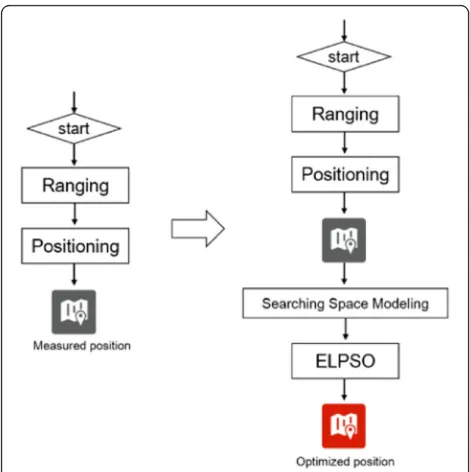
Figure 1 illustrates the major difference between the
proposed algorithm and existing work. Our key obser-vation is that it is hard to achieve perfect performance directly under traditional communication methods. Essen-tially, the main difficulty arises from the large gap between measured target and true target due to the limitation of hard devices and environmental barriers. The goal of our work is to bridge the gap by progressive optimization after communication measure. In the location step, we calcu-late the distance from bases to target by two-way ranging (TWR) and use TODA to estimate the target position. In the optimization step, we model the target area based on the pre-measured location and allocate multiple particles into the area to mine confident candidates. We then use ensemble learning particle swarm optimization (ELPSO) to fine-tune the measured target, resulting in a more
precise target position after optimization. In our proposed ELPSO algorithm, three different kinds of PSO variants, namely global PSO (GPSO), local PSO (LPSO), and bare bones PSO (BBPSO), are hybridized to complement each other. GPSO is used to accelerate convergence speed. LPSO is used to ensure rich population diversity. BBPSO is used to avoid complex parameter adjustments.
The proposed ELPSO algorithm addresses the drawbacks from prior work in three aspects: (1) Our algorithm attempts to achieve the global optimal from multiple populations with super best guide. This strat-egy aims at drawing advantages and potential charac-teristics together from different PSO algorithms, leading to an ensemble approach for progressive optimization in UWB indoor localization system. (2) Our location step uses UWB technique to predict the indoor target position in real time. This step aims at estimating an initial position within a certain margin of error, providing more discriminative searching space for ELPSO. (3) Our optimization step using ELPSO fine-tunes the measured location such that it can find the optimal with the highest precision, especially for 3D indoor localization.
We make the following three contributions in this work:
We propose to use progressive optimization for UWB indoor localization by ELPSO. We show that this strategy is crucial for good performance.
Our hardware communication-based method helps filter the target area, and our progressive optimization step helps find the most likely optimal point among the modeling area for indoor positioning task.
We present detailed evaluations for ELPSO and performance both in 2D and 3D UWB indoor positioning. Experimental results demonstrate that our ELPSO algorithm performs favorably against the state-of-the-art evolutionary computation methods. Our two-step location and optimization method achieves promising accuracy on UWB indoor positioning, surpassing the initial performance obviously.
The reminder of this paper is organized as follows.
Section 2 presents related work about particle swarm
optimization and indoor positioning, followed by a
de-tailed description about ELPSO algorithm in Section 3.
In Section4, we apply the proposed strategy into indoor positioning scenarios, i.e., both two dimensions and three dimensions. Moreover, we evaluate both ELPSO al-gorithm and its application in UWB indoor positioning by extensive experiments in Section5. Finally, a conclu-sion is given in the last section.
2 Related work
2.1 Particle swarm optimization
Particle swarm optimization (PSO) is a population-level intelligent algorithm firstly proposed by Kennedy and Eberhart in 1995 [8,9], which is originally from artificial intelligence and evolutionary computation theory,
fol-lowing birds’ searching behavior to achieve the global
optimum through collective collaboration. The research of PSO is an integration of various disciplines such as arti-ficial life, evolutionary computation, swarm intelligence, biology, and social psychology. Imagine a group of birds searching for food at random, suppose there is one and only one piece of food in a particular area, and none of the birds know where the food is. But they know how far they are from food. The simplest and most effective strat-egy to find food is to search the region around the nearest bird. We can model this optimization problem mathemat-ically. Given a flock of birds, say N birds, each bird is abstracted as a particle with no mass, volume but position
and velocity, which corresponds to the population of N
particles and extends to D dimensional space. The
pos-ition of the particleiin theNdimensional space is repre-sented as the vectorXi= [xi has a fitness value determined by the evaluation function and knowing its personal best position (pbest) so far and the current locationXi, which is the personal experience from itself. In addition, each particle has been kept known the best location (gbest) found by the entire population so far, which is the global experience from other peers. The particle determines the next movement by the best experience from its own or peers, then updating the corresponding velocity and location.
In the progress of particle swarm optimization re-search, scholars have made a lot of outstanding work in both theoretical study and practical application. Accord-ing to research focus and trend in recent years, the theoretical study of PSO could mainly be divided into four categories, namely single objective continuous space optimization problem, multiple objectives continuous space optimization problem, single objective discrete space optimization problem, and multiple objectives discrete space optimization problem.
For single objective continuous space optimization
problem [10], on the one hand, the movement behaviors
or patterns of particle swarm and individual particle are carried on the thorough discussion. Lu et al. [11] studied the movement behavior of particle swarm based on co-operative control framework. Bonyadi and Michalewicz [12] studied the movement patterns of individual particle and suggested that two influencing factors of particle’s movement are the correlation among continuous posi-tions and the range of movement. On the other hand, traditional theoretical research has also been extended.
Bonyadi and Michalewicz [13,14] made specific analysis on the stability, local convergence, and transformation sensitivity of PSO. Helwig et al. [15] analyzed the influ-ence of different boundary handling techniques on PSO.
For multiple objectives continuous space optimization
problem, Zhan et al. [16] proposed a co-evolutionary
technique for multiple objectives optimization problem. Subsequently, Hu et al. [17, 18] proposed a two-stage multiple objectives PSO algorithm based on parallel unit coordinate system. In addition to the uncon-strained optimization problem, there is also work in-volved in the multiple objectives optimization problem under constrained condition [19].
It is worth noting that discrete space optimization problem has aroused widespread study interest especially in the algorithm proposals for specific applications because many applications encountered in real world are combinatorial optimization problems, which can be characterized into discrete space optimization problem. However, the related representative work is not very abun-dant. For single objective discrete space optimization
problem, Wu et al. [20] proposed a discrete PSO
algo-rithm for covering array generation in the application of software combination test. For multiple objectives
discrete space optimization problem, Gong et al. [21]
proposed a decomposition-based multi-objective discrete PSO algorithm for complex network clustering.
The theoretical research of particle swarm optimization is rather extensive; meanwhile, applications of PSO are also deeply penetrating into various domains such as industrial engineering, machinery, communication, and bioscience. For instance, there are many applica-tions about power [22–24], electromagnetic [25, 26], and antenna [27–29] in the field of industrial engineer-ing. The most popular applications in machinery are tra-jectory optimization [30], defect classification [31,32], and
scheduling problems [33, 34]. Applications in
com-munication consist of routing optimization [35],
wireless communication system optimization [36],
filter design optimization [37], etc. Relatively, there are very limited study or applications in biology [38], arti-ficial intelligence [39, 40], and some other crossing fields [41–43]. In this work, we focus on the area of artificial intelligence and propose a novel PSO algorithm applied in UWB indoor localization.
2.2 Indoor positioning
Traditional indoor localization principles can be di-vided into three categories: geometry-based principle, fingerprint-based principle, and image-based principle. Based on the principle of geometry, indoor
position-ing technology can divided into WIFI [1], Bluetooth
[2], ultra-wideband [3], optical communication [4],
calculate the current position of the target by measur-ing the distance between the target and several fixed base stations. This kind of technology needs to be up-dated in real time. Based on the fingerprint principle, indoor positioning technology can be divided into
WIFI fingerprint localization [7] and geomagnetic
localization [44], and its principle is to collect some physical eigenvalues of different positions in the room in advance, and then drawing the fingerprint map, fi-nally locates the eigenvalue of the target measured directly, and compares with the fingerprint maps. This kind of technology needs to be collected in advance and updated regularly. Based on the image principle, indoor positioning technology can be divided into laser SLAM
positioning [45] and machine vision positioning [46], and its principle is to model the indoor scene with laser radar or camera and then using machine vision matching algo-rithm to estimate location. This kind of technology requires a large amount of computation for specific sce-narios. In the past decades, many approaches have been developed based on the above principles. We observe substantial applications of these approaches in indoor
localization. However, there are not yet perfect
solutions to balance accuracy, installation and oper-ation, and ease of use. Our work involves artificial intelligence, electronic communication, and evolution-ary computation. Examples include 2D and 3D UWB indoor positioning.
3 Ensemble learning particle swarm optimization
3.1 PSO variants employed in ELPSO
In the proposed ELPSO algorithm, GPSO, LPSO, and BBPSO are employed. The population is divided into three subpopulation groups in equal. When searching for the global optimum in a hyperspace, the particles benefit from guiding rules flying and searching more effectively and efficiently. In term of the typical PSO, the rules are the mechanisms of learning from a parti-cle’s historical best experience and its neighborhood’s best experience. Based on the manners of choosing the neighborhood’s best experience, PSO algorithms are originally categorized into GPSO (global version) and LPSO (local version). For GPSO, a particle takes the best particle’s experience in global as the neighbor-hood’s experience. For LPSO, a particle’s neighborhood experience is chosen from the best particle in experi-ence among particles in its local neighborhood defined by a topological structure. Beyond that, bare bones PSO (BBPSO) was proposed to improve precision while re-ducing the complexity of parameter tuning. In compari-son with GPSO and LPSO, BBPSO cancels the velocity item. Moreover, its position of the particle is directly obtained by random sampling of the Gaussian distribu-tion. Integrating the above three algorithms together enables our ELPSO algorithm preserves the diversity of population while discouraging premature convergence synchronously.
3.2 ELPSO with super best guide
As mentioned above, our ELPSO algorithm includes GPSO, LPSO, and BBPSO. For guiding rules, we add an ensemble learning component that learns from different
subpopulations’ social experience named as superbest.
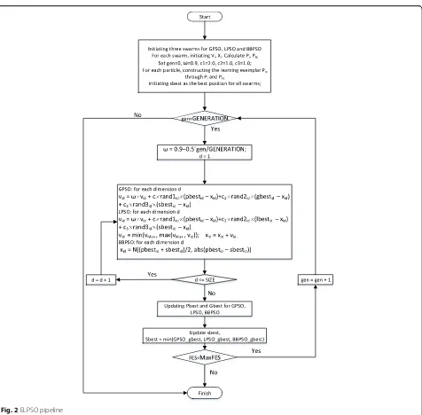
The superbest are selected from all three gbest and updated asynchronously. The corresponding velocity for each PSO variant also adopt new update rule. The new rule is as follows:
vi¼wviþc1 rand1iðpbesti−XiÞ þc2 rand2i gbesti−Xiþc3 rand3iðsuperbesti−XiÞ
ð1Þ
where c1= 1.49445, c2= 0.747225, and c3= 0.747225.
pbest is its own cognitive experience; gbest is its social component; the best experience found so far by its own subpopulation and super best is the best social experi-ence from the whole population. The flowchart of ELPSO is shown in Fig.2.
4 UWB indoor localization method using ELPSO
4.1 UWB indoor localization system design
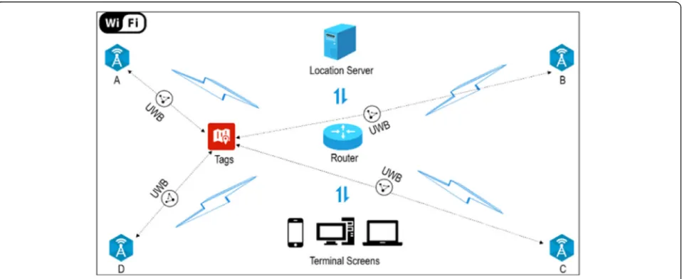
A lot of advances are developed for indoor wireless localization. A potential one is UWB technology by utilizing a narrow pulse to estimate the position of a tag. Only transmitted base-band pulse or an AM-modulated pulse can be used in a UWB-based sys-tems. The system proposed in this paper consists of an active tag, four base stations, a router, a location server, and several display terminals. The system with four base stations can theoretically cover the range of tens of thousands of square meters. Increasing the number of base stations, the positioning scene can be expanded further. The tag sends an ultra-wideband signal in a fixed time slot; each base station intercepts this signal, calling the ranging algorithm to get the
distance between base stations and the tag. After that, the distance information is transmitted in a wireless way to the location server through a router. Finally, the location server calls the localization algorithm to locate the tag and sends real-time positioning results to the terminals for display. Time of arrival (ToA) or time difference of arrival (TDoA) algorithm is usually used to triangulate its position. The structure of in-door positioning system proposed in this paper is shown in Fig. 3.
4.2 Ranging algorithm
Distance ranging is the first step in ultra-wideband
po-sitioning. Two-way ranging (TWR) [47] can be used to
calculate the distance by determining the flight time of signals between two objects. The distance between base stations and tag is achieved by the speed of radio waves multiplied by the time of signal flight. However, the clock offset can cause a larger margin of error [48, 49]; we design the ranging algorithm based on TWR as fol-lows. Firstly, we adopt the ultra-wideband wireless
trans-ceiver module DWM1000 produced by company
DecaWave [50] in our system. Then, given two
DWM1000 modules denoted by device A and device B re-spectively, device A can initiate ranging requests as the
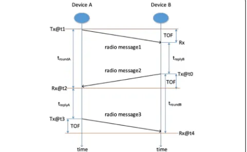
initiator of the distance ranging. Device B can listen and respond the radio message from device A as a responder. The ranging process is listed as Fig.4.
When device A sends a radio message to device B and records its sending time stamp as t1, device B re-ceives the message and sends a reply to device A
after a particular delay of treplyB. Device A receives
the reply and records the receiving time stamp as t2. To reduce the error caused by the clock offset, device A sends a radio message to device B again in a
spe-cific delay treplyA and records its own sending time
stamp as t3, and finally, device B receives the mes-sage and records a receiving time stamp as t4. In this way, using t1 and t2, device A can calculate its round trip time troundA; using t0 and t4, device B can calcu-late its round trip time troundB. So the time of flight (TOF) can be calculated by formula 1.
TOF¼troundA−troundBþtreplyA−treplyB
4 ð2Þ
If the speed of radio waves in the air is equal to the speed of lightc, the distanceRbetween A and B can be calculated by the following formula:
R¼cTOF¼ctroundA−troundBþtreplyA−treplyB
4
ð3Þ
4.3 Localization algorithm
At present, time difference of arrival (TDoA) [51] is
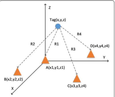
often used to realize ultra-wideband positioning. Assum-ing that there are four fixed base stations in the three-dimensional space, the position of the tag is (x,y,z), the position of the ith base station is (xi, yi, zi), and the distance between the tag and the base station is Ri(i= 1, 2,…,N,N= 4). The three-dimensional positioning
distri-bution diagram based on TDOA is shown in Fig.5.
The specific calculation process of TDOA localization algorithm is as follows. Firstly, the arrival time between the tag and each base station can be obtained from ran-ging algorithm illustrated previously; the difference be-tween every two arrival times is TDOA measured value. Then, we can calculate the difference between the tag and every two base stations according to TDOA mea-sured value. Multiple TDOA meamea-sured values of dis-tance differential equations constitute a two-surface system for the target position. Finally, the measured pos-ition of the tag can be obtained by solving the equation system.
4.4 ELPSO-based system implementation
System implementation includes hardware and software. In the hardware implementation part, the circuit is designed for the base stations and the tag. And the
ultra-wideband ranging communication program is com-pleted. The base stations and the tag all adopt the STM32103RC chip as the control unit and DWM1000 module as the ultra-wideband wireless transceiver. Each base station has an extra Wi-Fi module called ESP8266
Fig. 53D positioning based on TDOA. Points A, B, C, and D are represented as four fixed base stations, the tag sends an ultra-wideband signal in a fixed time slot, and each base station intercepts this signal, calling the ranging algorithm to get the distance between base stations and the tags
Fig. 6The tag. The tag adopts the STM32103RC chip as the control unit, and it contains DWM1000 module as the ultra-wideband wireless transceiver
than the tag, which is used to connect with the server. For ultra-wideband ranging communication program, transmission data rate is set to 110 kbps, the center fre-quency of channel is 3993.6 MHz, and the bandwidth is 499.2 MHz. The details of tag and base stations are
shown in Figs. 6 and 7. In the software implementation
part, based on the Android platform, the location server
program was designed and the indoor positioning app was developed. The working scenes can be updated through Wi-Fi network automatically.
5 Experimental results and discussion
A set of experiments was conducted to verify the per-formance of the proposed algorithm ELPSO and its application in UWB indoor localization. The competitors consist of three individual PSO embedding in ELPSO and another four famous PSO variants in the literature. Moreover, both 2D and 3D real-time test prove effect-ive in UWB indoor localization using evolutionary computation strategy.
5.1 Experimental results for ELPSO
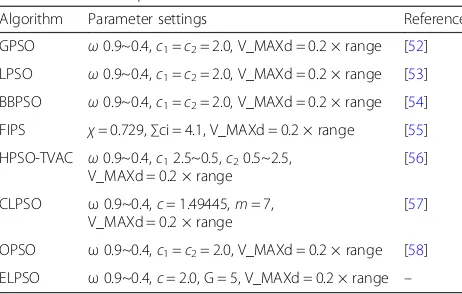
To demonstrate the efficiency of the proposed ELPSO, the competitors are listed in Table 1in details. Also, we applied 14 benchmark functions listed in Table2in this
section. These functions (CEC2005) https://www.lri.fr/
~hansen/cec2005.html are widely used to evaluate PSO algorithms. To be fair, for all eight PSO algorithms, the
Table 1PSOs compared
Algorithm Parameter settings Reference
GPSO ω0.9~0.4,c1=c2= 2.0, V_MAXd = 0.2 × range [52]
LPSO ω0.9~0.4,c1=c2= 2.0, V_MAXd = 0.2 × range [53]
BBPSO ω0.9~0.4,c1=c2= 2.0, V_MAXd = 0.2 × range [54]
FIPS χ= 0.729,∑ci = 4.1, V_MAXd = 0.2 × range [55]
HPSO-TVAC ω0.9~0.4,c12.5~0.5,c20.5~2.5, V_MAXd = 0.2 × range
[56]
CLPSO ω0.9~0.4,c= 1.49445,m= 7, V_MAXd = 0.2 × range
[57]
OPSO ω0.9~0.4,c1=c2= 2.0, V_MAXd = 0.2 × range [58]
ELPSO ω0.9~0.4,c= 2.0, G = 5, V_MAXd = 0.2 × range –
Table 2Functions tested
Test function D Search space fmin Acceptance Name
Unimodal 30 [−100,100]D 0 0.01 Sphere
30 [−10,10]D 0 0.01 Schwefel’s P2.22
30 [−10,10]D 0 100 Rosenbrock
30 [−1.28,1.28]D 0 0.01 Quadric noise
Multimodal 30 [−500,500]D −12,569.5 −10,000 Schwefel
30 [−5.12,5.12]D 0 50 Rastrigin
30 [−32,32]D 0 0.01 Ackley
30 [−600,600]D 0 0.01 Griewank
30 [−50,50]D 0 0.01 Generalized
Penalized
30 [−50,50]D 0 0.01
Rotated 30 [−500,500]D −12,569.5 −8000 Rotated Schwefel
30 [−5.12,5.12]D 0 100 Rotated Rastrigin
30 [−32,32]D 0 1 Rotated Ackley
Table 3Performance for ELPSO and other PSOs
Functions GPSO LPSO FIPS HPSO-TVAC CLPSO OPSO BBPSO ELPSO
f1 Mean 1.69 × 10⁻³¹ 4.48 × 10⁻¹⁴ 5.55 × 10⁻¹⁴ 2.55 × 10⁻³³ 2.54 × 10⁻¹² 5.33 × 10⁻¹⁸ 1.90 × 10−53 5.15 × 10−38
Std. Dev 4.55 × 10⁻³¹ 4.00 × 10⁻¹⁴ 2.26 × 10⁻¹⁴ 5.55 × 10⁻³³ 8.84 × 10⁻¹³ 3.86 × 10⁻¹⁸ 3.69 × 10−53 9.64 × 10−38
Rank 4 6 7 3 8 5 1 2
f2 Mean 1.30 × 10⁻²¹ 1.97 × 10⁻¹⁰ 1.48 × 10⁻⁸ 8.44 × 10⁻²⁰ 3.59 × 10⁻⁸ 1.76 × 10⁻¹⁰ 1.52 × 10⁻²⁹ 7.44 × 10⁻²²
Std. Dev 1.83 × 10⁻²¹ 9.85 × 10⁻¹¹ 4.04 × 10⁻⁹ 8.21 × 10⁻²⁰ 9.21 × 10⁻⁹ 1.52 × 10⁻¹⁰ 2.24 × 10⁻²⁹ 5.49 × 10⁻²²
Rank 3 6 7 4 8 5 1 2
f3 Mean 36.94197 22.39326 24.71584 19.28725 14.1712 41.60198 37.72958 1.83494
Std. Dev 25.53545 10.8901 0.24099 4.70946 10.72737 28.6714 40.18926 6.57884
Rank 6 4 5 3 2 8 7 1
f4 Mean 0.00851 0.01911 0.00377 0.05747 0.00595 0.05798 0.0102 0.01484
Std. Dev 0.00328 0.00481 8.57 × 10⁻⁴ 0.02237 0.00153 0.02131 0.00349 0.00391
Rank 3 6 1 7 2 8 4 5
f5 Mean −10,000.1 −9594.07 −9280.09 −10,931.9 −12,569.5 −10,336.8 −12,218.8 −12,569.5
Std. Dev 479.961 376.9293 906.5758 374.6448 0 501.6225 185.7255 0
Rank 6 7 8 4 1 5 3 1
f6 Mean 29.72935 33.18402 38.25496 6.80555 7.61 × 10⁻⁵ 6.08918 1.19395 0
Std. Dev 8.41469 6.85435 8.58552 2.67412 7.16 × 10⁻⁵ 2.28549 1.1124 0
Rank 6 7 8 5 2 4 3 1
f7 Mean 1.34 × 10⁻¹⁴ 1.18 × 10⁻⁷ 1.09 × 10⁻⁷ 8.54 × 10⁻¹⁴ 5.29 × 10⁻⁷ 5.87 × 10⁻⁹ 8.12 × 10⁻¹⁵ 4.28 × 10⁻¹⁵
Std. Dev 2.90 × 10⁻¹⁵ 9.11 × 10⁻⁸ 2.75 × 10⁻⁸ 4.70 × 10⁻¹⁴ 1.54 × 10⁻⁷ 1.89 × 10⁻⁹ 2.13 × 10⁻¹⁵ 7.11 × 10⁻¹⁶
Rank 3 7 6 4 8 5 2 1
f8 Mean 0.00837 0.00227 2.19 × 10⁻⁶ 0.00325 1.23 × 10⁻⁸ 0.00118 0.00404 0
Std. Dev 0.00996 0.00432 1.10 × 10⁻⁵ 0.00419 1.86 × 10⁻⁸ 0.00277 0.00721 0
Rank 8 5 3 6 2 4 7 1
f9 Mean 0.00415 1.74 × 10⁻¹⁵ 3.70 × 10⁻¹⁶ 1.77 × 10⁻²⁹ 1.03 × 10⁻¹³ 1.27 × 10⁻¹⁹ 1.61 × 10⁻³² 1.57 × 10⁻³²
Std. Dev 0.02073 3.08 × 10⁻¹⁵ 2.52 × 10⁻¹⁶ 8.17 × 10⁻³⁰ 6.16 × 10⁻¹⁴ 1.14 × 10⁻¹⁹ 1.43 × 10⁻³³ 0
Rank 8 6 5 3 7 4 2 1
f10 Mean 0.00176 1.78 × 10⁻¹³ 5.55 × 10⁻¹⁵ 2.44 × 10⁻²⁸ 2.17 × 10⁻¹² 1.06 × 10⁻¹⁸ 1.43 × 10⁻³² 1.35 × 10⁻³²
Std. Dev 0.00411 2.55 × 10⁻¹³ 2.42 × 10⁻¹⁵ 1.08 × 10⁻²⁸ 1.11 × 10⁻¹² 6.37 × 10⁻¹⁹ 3.94 × 10⁻³³ 2.47 × 10⁻³⁴
Rank 8 6 5 3 7 4 2 1
f11 Mean −8840.69 −9880.77 −7430.41 −8515.69 −9377.81 −9700.32 −10,697.7 −10,597.2
Std. Dev 1114.708 1240.53 1303.977 1818.807 870.6272 1423.02 1652.89 2096.313
Rank 6 3 8 7 5 4 1 2
f12 Mean 56.75235 49.65696 118.3976 32.59482 77.63228 73.04538 42.86277 56.53254
Std. Dev 13.11957 11.62829 19.42732 9.56176 10.19121 19.79576 11.10137 14.19207
Rank 5 3 8 1 7 6 2 4
f13 Mean 1.72364 1.23822 1.34 × 10⁻⁷ 5.71977 9.49 × 10⁻⁶ 1.45 × 10⁻⁸ 7.84 × 10⁻¹⁵ 4.28 × 10⁻¹⁶
Std. Dev 0.77477 0.66329 3.72 × 10⁻⁸ 1.51541 2.58 × 10⁻⁵ 6.46 × 10⁻⁹ 1.62 × 10⁻¹⁵ 7.11 × 10⁻¹⁶
Rank 7 6 4 8 5 3 2 1
f14 Mean 0.01496 0.00202 3.89 × 10⁻⁹ 0.01201 2.98 × 10⁻⁵ 0.00118 2.96 × 10⁻⁴ 5.47 × 10⁻⁹
Std. Dev 0.01319 0.00506 9.01 × 10⁻⁹ 0.01348 3.32 × 10⁻⁵ 0.00327 0.00148 1.60 × 10⁻⁸
Rank 8 6 2 7 3 5 4 1
Average rank 5.79 5.57 5.50 4.64 4.79 5.00 2.93 1.71
population size is the same, equal to 40; the maximum number of function evaluations (FEs) is set to 2 × 10⁵. Note that the number of FEs is equally divided into three parts for three swarms used in ELPSO. To eliminate statistical errors, the test for each algorithm and each function will repeat 25 times independently for achieving average results to compare.
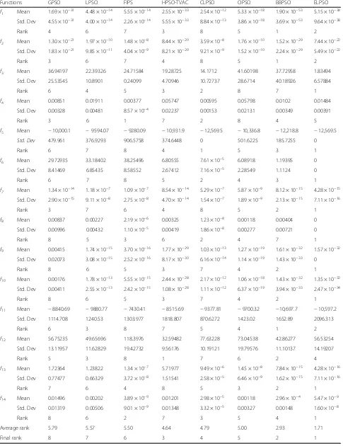
The performance for ELPSO algorithm compared with
other competitors are shown in Table 3. The mean and
the standard deviation of the solutions are provided. It can be observed that the ELPSO achieves the best solu-tion on funcsolu-tions f3,f5,f6, f7, f8,f9,f10, andf13. Although
FIPS performs best on the noise function (f4) and
HPSO-TVAC yields the best solution on the rotated Rastrigin’s function (f12), the ELPSOs can also achieve
comparable results on these two functions. Table 3 also
ranks the algorithms on performance in terms of the
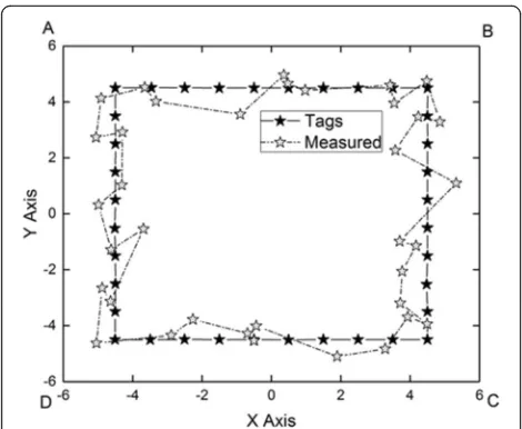
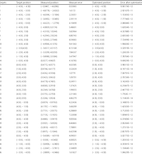
Fig. 82D indoor localization configuration. In this experiment, there are 36 targets supposed to localize in two-dimensional space, which are represented by black pentagonal stars. Then, we achieve 36 promising position measured by communication method mentioned in Section4. The measured results are denoted by white pentagonal stars. The specific location coordinates are listed in Table4
Fig. 92D indoor localization modeling and optimization. After the initial measurement, for every target, we first establish the search space based on the corresponding measured target; then, we optimize the measured target by our proposed ELPSO algorithm to achieve the optimal localization, which is represented by the red pentagonal stars. The specific location coordinates are listed in Table4
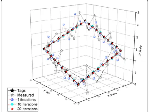
Fig. 10Results of 10 iterations for 2D indoor localization. We illustrate the optimized position for each target after 10 iterations, which is denoted by the red dots. It can be found that the locations are not optimal because the ELPSO algorithm have not
converge yet
mean solution accuracy. It can be observed that ELPSO offers the highest performance overall.
Experimental comparisons verify that the sbest param-eter indeed help the ELPSO perform better than the traditional PSOs and most existing improved PSO vari-ants on almost all test functions in solving global optimization problems. The ELPSO offer not only a better performance in global optimization, but also a finer-grain search ability, owing to the sbest parameter
that could preserve and utilize the most useful informa-tion from three different swarms based on different characteristics.
5.2 Experimental results for 2D UWB localization
In the second phase of the experiments, we model the search space based on every measured target through traditional UWB localization method elaborated in Section4. Suppose a square area 10 m × 10 m, there are
Table 4Performance of 2D indoor localization using ELPSO
Targets Target position Measured position Measure error Optimized position Error after optimization
1 (−4.50,−4.50) (−5.0447,−4.6286) 0.55965 (−4.50,−4.50) 9.96174E−12
2 (−4.50,−3.50) (−4.8778,−2.6532) 1.6172 (−4.50,−3.50) 2.92107E−11
3 (−4.50,−2.50) (−4.6396,−3.1304) 2.23051 (−4.50,−2.50) 1.15305E−13
4 (−4.50,−1.50) (−3.6902,−0.5405) 2.39119 (−4.50,−1.50) 7.77746E−12
5 (−4.50,−0.50) (−4.6223,−1.2778) 4.19499 (−4.50,−0.50) 2.08048E−13
6 (−4.50, 0.50) (−4.9839, 0.3174) 5.48691 (−4.50, 0.50) 1.62034E−12
7 (−4.50, 1.50) (−4.3102, 1.0244) 5.82964 (−4.50, 1.50) 4.33788E−12
8 (−4.50, 2.50) (−4.2943, 2.9224) 6.80743 (−4.50, 2.50) 2.60556E−13
9 (−4.50, 3.50) (−5.0565, 2.7348) 8.59065 (−4.50, 3.50) 7.72499E−14
10 (−4.50, 4.50) (−4.9066, 4.1376) 9.41363 (−4.50, 4.50) 1.96826E−11
11 (−3.50,4.50) (−3.6517, 4.5157) 8.15168 (−3.50,4.50) 3.32919E−12
12 (−2.50, 4.50) (−3.3290, 4.0250) 7.84337 (−2.50, 4.50) 1.22653E−12
13 (−1.50, 4.50) (−0.8980, 3.5584) 5.47947 (−1.50, 4.50) 7.78704E−13
14 (−0.50, 4.50) (0.3577, 4.9607) 4.16783 (−0.50, 4.50) 9.69029E−12
15 (0.50, 4.50) (0.4772, 4.6571) 4.02585 (0.50, 4.50) 3.98315E−13
16 (1.50, 4.50) (0.9746, 4.4177) 3.52639 (1.50, 4.50) 8.19715E−14
17 (2.50, 4.50) (3.4262, 4.5936) 1.0779 (2.50, 4.50) 7.04791E−12
18 (3.50, 4.50) (3.5423, 3.9632) 1.09791 (3.50, 4.50) 2.70726E−12
19 (4.50, 4.50) (4.4778, 4.7481) 0.24911 (4.50, 4.50) 3.14245E−12
20 (4.50, 3.50) (4.8583, 3.2910) 1.37425 (4.50, 3.50) 6.21847E−12
21 (4.50, 2.50) (4.2349, 3.4760) 1.99055 (4.50, 2.50) 2.44775E−11
22 (4.50, 1.50) (3.5755, 2.2703) 2.21383 (4.50, 1.50) 1.7763E−11
23 (4.50, 0.50) (5.3266, 1.0924) 4.86279 (4.50, 0.50) 5.11463E−14
24 (4.50,−0.50) (3.6974,−0.9763) 4.22436 (4.50,−0.50) 3.14801E−13
25 (4.50,−1.50) (4.1707,−1.1405) 5.68209 (4.50,−1.50) 1.42503E−11
26 (4.50,−2.50) (3.7731,−2.0575) 6.28869 (4.50,−2.50) 3.71205E−12
27 (4.50,−3.50) (3.7135,−3.1925) 7.22008 (4.50,−3.50) 1.00981E−12
28 (4.50,−4.50) (4.4883,−3.9419) 9.00566 (4.50,−4.50) 6.37406E−12
29 (3.50,−4.50) (3.9301,−3.6926) 8.46865 (3.50,−4.50) 2.06266E−12
30 (2.50,−4.50) (3.2818,−4.8317) 7.78891 (2.50,−4.50) 1.27315E−12
31 (1.50,−4.50) (1.8975,−5.1044) 6.42598 (1.50,−4.50) 2.85797E−12
32 (0.50,−4.50) (−0.4389,−4.0119) 4.09031 (0.50,−4.50) 3.02775E−12
33 (−0.50,−4.50) (−0.500,−4.5402) 4.00025 (−0.50,−4.50) 1.20355E−13
34 (−1.50,−4.50) (−0.6906,−4.2803) 3.81578 (−1.50,−4.50) 4.35941E−14
35 (−2.50,−4.50) (−2.2647,−3.7811) 2.34809 (−2.50,−4.50) 1.13464E−12
four base stations A(xA,yA) = (−5, 5), B(xB,yB) = (5, 5), C(xC,yC) = (−5,−5), and D(xD,yD) = (5,−5) located in it. The configuration of 2D indoor localization is shown in Fig.8. All the positions of targets are supposed uniform distribution; we test 36 targets in this paper.
For every target, the steps of optimization are as follows: Step 1: Swarm initiation—there are three swarms used in ELPSO algorithm; the total number of particles is N, indexed byi= 1....N,D= 2;
Step 2: Position measuring—according to the TWR al-gorithm and improved TODA alal-gorithm presented in Section4, we can initially measure the position of tag to base station;
Step 3: Searching space—based on the measured pos-ition in the previous step, creating a spherical space with
a radius of 50 cm. N particles are all included in this
space; both moving space and search space of all parti-cles should not exceed this range;
Step 4: Fitness calculation—after achieving the
dis-tance L from each particle to each base station, given
the measured distance R from target to each base
Fig. 123D indoor localization configuration. In this experiment, there are 36 targets supposed to localize in three-dimensional space, which are represented by black pentagonal stars. Then, we achieve 36 promising position measured by communication method mentioned in Section4. The measured results are denoted by white pentagonal stars. The specific location coordinates are listed in Table5
Fig. 133D indoor localization modeling. After the initial measurement, for every target, we first establish the search space based on the corresponding measured target similar to 2D configuration. The only difference is that we model the searching space in three dimensions this time, which is denoted by a green sphere. The swarm are initiated and randomly distributed in this sphere
Fig. 143D indoor localization optimization. After modeling, we optimize the measured target by our proposed ELPSO algorithm to achieve the optimal localization, which is represented by the red dots. The specific localization coordinates are listed in Table5
station, for the i_th particle and the j_th target, here, we have the fitness function listed as follows:
fð Þ ¼Pi LiA−R j A
2
þ Li B−R
j B
2
þ Li C−R
j C
2
þ Li D−R
j D
2
ð4Þ
When f= 0, Pi achieved the optimal solution, i.e., Pi
exactly located in the position of target. The
corresponding modeling and optimization of 2D
in-door localization are shown in Fig. 9. We find that
the fitness function could approach convergence after 20 iterations, which appeals to the demand of real time. The results after 10 iterations and 20 iterations for 2D indoor localization are shown in Figs. 10and 11, respectively. The corresponding experimental results are listed in Table4. It can be found that after optimization, the positioning accuracy is obviously improved. This is
Table 5Performance of 3D indoor localization using ELPSO
Targets Target position Measured position Measure error Optimized position Error after optimization
1 (−4.50,−4.50,3.60) (−4.8963,−3.9034,2.7739) 1.195549 (−4.5001,−4.4999,3.6000) 1.36E−07
2 (−4.50,−3.50,3.40) (−3.7988,−3.2387,3.1449) 0.222615 (−4.4997,−3.4998,3.4010) 4.47E−07
3 (−4.50,−2.50,3.20) (−5.4980,−3.1084,4.1273) 10.21776 (−4.4999,−2.4997,3.2001) 4.79E−07
4 (−4.50,−1.50,3.00) (−4.5462,−0.8003,2.2173) 10.38149 (−4.4999,−1.5000,3.0001) 9.33E−07
5 (−4.50,−0.50,2.80) (−4.2680,−1.1158,3.4165) 14.95691 (−4.4999,−0.4999,2.7997) 2.81E−08
6 (−4.50,0.50,2.60) (−5.0689,0.0609,2.3528) 31.26613 (−4.4995,0.4998,2.6004) 8.35E−07
7 (−4.50,1.50,2.40) (−4.4801,1.9412,3.0769) 36.41482 (−4.4999,1.4999,2.3998) 1.02E−06
8 (−4.50,2.50,2.20) (−3.8865,2.6628,2.7892) 41.16078 (−4.5004,2.4999,2.2002) 6.60E−07
9 (−4.50,3.50,2.00) (−4.4704,2.5495,1.8709) 64.44693 (−4.5003,3.5000,1.9997) 3.14E−07
10 (−4.50,4.50,1.80) (−4.4249,5.4920,1.1801) 81.02231 (−4.4992,4.5003,1.8004) 7.19E−08
11 (−3.50,4.50,1.60) (−4.3540,5.3446,1.2056) 79.2619 (−3.4990,4.5001,1.6009) 3.73E−08
12 (−2.50,4.50,1.40) (−1.5197,5.4871,2.3420) 38.0984 (−2.4999,4.4997,1.3999) 3.49E−07
13 (−1.50,4.50,1.20) (−1.8102,3.5861,0.7940) 40.8185 (−1.5000,4.5004,1.2001) 6.35E−08
14 (−0.50,4.50,1.00) (−1.3398,4.7150,0.9666) 34.15083 (−0.4997,4.5001,1.0001) 1.06E−07
15 (0.50,4.50,0.80) (0.9290,4.7708,−0.1517) 13.73123 (0.4999,4.5010,0.8008) 1.54E−07
16 (1.50,4.50,0.60) (0.8956,5.4528,0.2310) 14.03577 (1.5003,4.4998,0.6007) 2.97E−07
17 (2.50,4.50,0.40) (2.1190,3.5713,1.0994) 7.02079 (2.5003,4.5007,0.4004) 2.14E−07
18 (3.50,4.50,0.20) (3.4177,5.3572,−0.7132) 2.739887 (3.5000,4.4999,0.2004) 2.48E−07
19 (4.50,4.50,0.00) (3.5646,4.8827,0.0601) 1.024956 (4.5001,4.5003,0.0000) 4.13E−08
20 (4.50,3.50,0.20) (3.5194,4.2055,0.2805) 0.504606 (4.4999,3.5004,0.1998) 5.50E−07
21 (4.50,2.50,0.40) (5.1754,2.1557,1.0299) 7.673302 (4.5002,2.4997,0.3994) 2.57E−07
22 (4.50,1.50,0.60) (4.7668,2.1279,0.9010) 11.15713 (4.5005,1.5004,0.6002) 1.33E−07
23 (4.50,0.50,0.80) (5.3860,−0.0327,0.5229) 24.2334 (4.4998,0.4998,0.8001) 5.92E−07
24 (4.50,−0.50,1.00) (3.6574,−0.8015,1.9427) 18.26336 (4.5001,−0.5000,1.0011) 9.60E−07
25 (4.50,−1.50,1.20) (4.3772,−1.7886,0.9126) 34.70706 (4.5003,−1.4994,1.2003) 4.18E−07
26 (4.50,−2.50,1.40) (4.0502,−1.8335,0.5315) 44.10311 (4.4997,−2.5002,1.3995) 3.88E−07
27 (4.50,−3.50,1.60) (4.7995,−2.5315,1.2096) 69.97281 (4.4996,−3.5003,1.6000) 2.74E−07
28 (4.50,−4.50,1.80) (3.6330,−3.5897,1.1721) 67.36877 (4.4997,−4.5002,1.8001) 6.72E−07
29 (3.50,−4.50,2.00) (3.4149,−4.9324,1.7673) 62.88624 (3.4992,−4.4994,1.9989) 7.84E−07
30 (2.50,−4.50,2.20) (3.4877,−5.2365,1.8627) 64.46026 (2.4996,−4.4999,2.1998) 1.28E−07
31 (1.50,−4.50,2.40) (1.9432,−4.4983,2.8564) 41.72338 (1.4996,−4.5004,2.4001) 3.70E−07
32 (0.50,−4.50,2.60) (−0.2560,−4.0642,3.0258) 18.38233 (0.5002,−4.5002,2.5993) 5.78E−07
33 (−0.50,−4.50,2.80) (−0.7117,−3.5567,2.5600) 15.29884 (−0.4996,−4.5003,2.8004) 1.17E−07
34 (−1.50,−4.50,3.00) (−1.6642,−4.2216,2.1823) 8.787994 (−1.4999,−4.4998,2.9990) 2.54E−08
35 (−2.50,−4.50,3.20) (−2.7616,−4.6484,3.3791) 3.076307 (−2.4997,−4.5002,3.2005) 1.58E−07
due to the use of ELPSO to optimize indoor positioning accuracy.
5.3 Experimental results for 3D UWB localization
3D UWB indoor localization is an extension of 2D. Simi-larly, suppose a cube region 10 m × 10 m × 10 m, there are four base stations A (xA,yA,zA) = (0, 0, 10), B (xB,yB,
zB) = (0,10, 10), C (xC,yC,zC) = (10,10, 10), and D (xD,yD,
zD) = (10, 0, 10) located in it in the same. The configur-ation of 3D indoor localizconfigur-ation is shown in Fig.12. The 36 target positions (x,y,z) are uniformly distributed dur-ing the test. For every target, the optimization step is consistent with the two-dimensional case.
The corresponding modeling and optimization of 3D in-door localization are shown in Figs.13and14, respectively. Note that the fitness function could also approach conver-gence after 20 iterations, as shown in Fig.15. The corre-sponding experimental results are listed in Table 5, which indicate that our indoor location method can overcome the problem of inaccurate 3D positioning.
6 Conclusions
In this paper, we propose the ELPSO, a particle swarm optimization algorithm composed of three variants of PSO under super best guide. The ensemble learning strategy proposed in this paper follows the philosophy that a particle learns not only from its own experience and its neighbors’ experience, but also from other swarms’ experience. This new learning strategy helps a particle construct a more promising and efficient guidance searching space, especially for optimizing indoor localization problem. It is thus ap-plied to both the 2D version and the 3D version of UWB indoor localization. For testing the performance of ELPSO, comprehensive experimental tests have been undertaken on widely used benchmark CEC2005. The results demon-strate a high effectiveness of the ELPSO, which significantly outperforming other existing PSO algorithms on most of the functions tested; for testing the performance of ELPSO applied in UWB indoor localization, 2D and 3D versions of UWB indoor localization tests have been conducted. The experimental results show that ELPSO plays an important role in UWB indoor localization, and the positioning accur-acy is remarkably improved after our optimization process. Future work will be continued to apply this kind of learning strategy into other indoor localization techniques.
The authors promise that all the experiments’ data
and results in this article will be true and valid.
Abbreviations
BBPSO:Bare bones PSO; EL: Ensemble learning; ELPSO: Ensemble learning particle swarm optimization; GPS: Global Position System; GPSO: Global PSO; LPSO: Local PSO; PSO: Particle swarm optimization; RFID: Radio frequency identification; TDoA: Time difference of arrival; ToF: Time of flight; TWR: Two-way ranging; UWB: Ultra-wideband
Acknowledgements
The research presented in this paper was partly supported by my dear teacher and friends in Wuhan University.
Authors’contributions
XC is the main writer of this paper. She proposed the main idea, deduced the performance of ELPSO, completed the experiment, and analyzed the result. LY introduced the idea of applying the proposed ELPSO algorithm into indoor localization. QZ gave some important suggestions for the paper. All authors read and approved the final manuscript.
Competing interests
The authors declare that they have no competing interests.
Publisher’s Note
Springer Nature remains neutral with regard to jurisdictional claims in published maps and institutional affiliations.
Received: 18 March 2018 Accepted: 26 April 2018
References
1. Ingram S J, Harmer D, Quinlan M. UltraWideBand indoor positioning systems and their use in emergencies[C]// Position Location and Navigation Symposium. IEEE, 2004:706-715.
2. M Hazas, A Hopper, Broadband ultrasonic location systems for improved indoor positioning. IEEE Trans. Mob. Comput.5(5), 536–547 (2006) 3. H Liu, H Darabi, P Banerjee, et al., Survey of wireless indoor positioning
techniques and systems. IEEE Trans Syst Man Cybernet Part C37(6), 1067– 1080 (2007)
4. Anastasi G, Bandelloni R, Conti M, et al. Experimenting an indoor bluetooth-based positioning service[C]//International Conference on Distributed Computing Systems Workshops, 2003. Proc IEEE, 2003:480-483. 5. MR Mahfouz, C Zhang, BC Merkl, et al., Investigation of high-accuracy
indoor 3-D positioning using UWB technology. IEEE Trans Microwave Theory Tech56(6), 1316–1330 (2008)
6. R Mendes, J Kennedy, J Neves, The fully informed particle swarm: simpler, maybe better. IEEE Trans. Evol. Comput.8(3), 204–210 (2004)
7. Yang Z, Wu C, Liu Y. Locating in fingerprint space: wireless indoor localization with little human intervention[C]// international conference on mobile computing and NETWORKING. ACM, 2012:269-280.
8. Kennedy J, Eberhart R. Particle swarm optimization[C]// IEEE International Conference on Neural Networks, 1995. Proceedings. IEEE, 2002:1942-1948 vol.4.
9. Eberhart R, Kennedy J. A new optimizer using particle swarm theory[C]// International Symposium on MICRO Machine and Human Science. IEEE, 2002:39–43.
10. MR Bonyadi, Z Michalewicz, Particle swarm optimization for single objective continuous space problems: a review. Evol. Comput.8, 1–54 (2016) 11. Q Lu, QL Han, S Liu, A cooperative control framework for a collective
decision on movement behaviors of particles. IEEE Trans. Evol. Comput. 20(6), 859–873 (2016)
12. MR Bonyadi, Z Michalewicz, Impacts of coefficients on movement patterns in the particle swarm optimization algorithm. IEEE Trans. Evol. Comput. 21(3), 378–390 (2017)
13. MR Bonyadi, Z Michalewicz, Analysis of stability, local convergence, and transformation sensitivity of a variant of the particle swarm optimization algorithm. IEEE Trans. Evol. Comput.20(3), 370–385 (2016)
14. MR Bonyadi, Z Michalewicz, Stability analysis of the particle swarm optimization without stagnation assumption. IEEE Trans. Evol. Comput. 20(5), 814–819 (2016)
15. S Helwig, J Branke, S Mostaghim, Experimental analysis of bound handling techniques in particle swarm optimization. IEEE Trans. Evol. Comput.17(2), 259–271 (2013)
16. ZH Zhan, J Li, J Cao, J Zhang, HSH Chung, YH Shi, Multiple populations for multiple objectives: a coevolutionary technique for solving multiobjective optimization problems. IEEE Trans Cybernet43(2), 445–463 (2013) 17. W Hu, GG Yen, G Luo, Many-objective particle swarm optimization using
18. W Hu, GG Yen, Adaptive multiobjective particle swarm optimization based on parallel cell coordinate system. IEEE Trans. Evol. Comput.19(1), 1–18 (2015) 19. AS Dymond, AP Engelbrecht, S Kok, PS Heyns, Tuning optimization
algorithms under multiple objective function evaluation budgets. IEEE Trans. Evol. Comput.19(3), 341–358 (2015)
20. H Wu, C Nie, FC Kuo, H Leung, CJ Colbourn, A discrete particle swarm optimization for covering array generation. IEEE Trans. Evol. Comput.19(4), 575–591 (2015)
21. M Gong, Q Cai, X Chen, L Ma, Complex network clustering by multiobjective discrete particle swarm optimization based on decomposition. IEEE Trans. Evol. Comput.18(1), 82–97 (2014) 22. K Maji, P Acharjee, Multiple solutions of optimal PMU placement using
exponential binary PSO algorithm for smart grid applications. IEEE Trans. Ind. Appl.53(3), 2550–2559 (2017)
23. J Zhao, F Wen, ZY Dong, Y Xue, KP Wong, Optimal dispatch of electric vehicles and wind power using enhanced particle swarm optimization. IEEE Trans Indust Inf8(4), 889–899 (2012)
24. S Nanchian, A Majumdar, BC Pal, Three-phase state estimation using hybrid particle swarm optimization. IEEE Trans Smart Grid8(3), 1035–1045 (2017) 25. JH Lee, JW Kim, JY Song, DW Kim, YJ Kim, SY Jung, Distance-based
intelligent particle swarm optimization for optimal design of permanent magnet synchronous machine. IEEE Trans. Magn.53(6), 1–4 (2017) 26. J Zhao, M Lin, D Xu, L Hao, W Zhang, Vector control of a hybrid axial field
flux-switching permanent magnet machine based on particle swarm optimization. IEEE Trans. Magn.51(11), 1–4 (2015)
27. W Xu, BY Duan, P Li, N Hu, Y Qiu, Multiobjective particle swarm optimization of boresight error and transmission loss for airborne radomes. IEEE Trans. Antennas Propag.62(11), 5880–5885 (2014)
28. ZD Zaharis et al., Exponential log-periodic antenna design using improved particle swarm optimization with velocity mutation. IEEE Trans. Magn.53(6), 1–4 (2017)
29. S Kibria, MT Islam, B Yatim, New compact dual-band circularly polarized universal RFID reader antenna using ramped convergence particle swarm optimization. IEEE Trans. Antennas Propag.62(5), 2795–2801 (2014) 30. JJ Kim, JJ Lee, Trajectory optimization with particle swarm optimization for
manipulator motion planning. IEEE Trans Indust Inf11(3), 620–631 (2015) 31. M Van, HJ Kang, Bearing defect classification based on individual wavelet local fisher discriminant analysis with particle swarm optimization. IEEE Trans Indust Inf12(1), 124–135 (2016)
32. M Van, HJ Kang, Wavelet kernel local fisher discriminant analysis with particle swarm optimization algorithm for bearing defect classification. IEEE Trans. Instrum. Meas.64(12), 3588–3600 (2015)
33. Y Wang, Y Shen, X Yuan, Y Yang, Operating point optimization of auxiliary power unit based on dynamic combined cost map and particle swarm optimization. IEEE Trans. Power Electron.30(12), 7038–7050 (2015) 34. HP Hsu, Solving feeder assignment and component sequencing problems
for printed circuit board assembly using particle swarm optimization. IEEE Trans. Autom. Sci. Eng.14(2), 881–893 (2017)
35. M Shen, ZH Zhan, WN Chen, YJ Gong, J Zhang, Y Li, Bi-velocity discrete particle swarm optimization and its application to multicast routing problem in communication networks. IEEE Trans. Ind. Electron.61(12), 7141–7151 (2014)
36. AA Minasian, TS Bird, Particle swarm optimization of microstrip antennas for wireless communication systems. IEEE Trans. Antennas Propag.61(12), 6214–6217 (2013)
37. YC Yun, SH Oh, JH Lee, K Choi, TK Chung, HS Kim, Optimal design of a compact filter for UWB applications using an improved particle swarm optimization. IEEE Trans. Magn.52(3), 1–4 (2016)
38. J Sun, V Palade, X Wu, W Fang, Multiple sequence alignment with hidden Markov models learned by random drift particle swarm optimization. IEEE/ ACM Trans. Comput. Biol. Bioinform11(1), 243–257 (2014)
39. SK Chou, MK Jiau, SC Huang, Stochastic set-based particle swarm optimization based on local exploration for solving the carpool service problem. IEEE Trans Cybernet46(8), 1771–1783 (2016)
40. W Hu, Y Tan, Prototype generation using multi-objective particle swarm optimization for nearest neighbor classification. IEEE Transa Cybernet46(12), 2719–2731 (2016)
41. K Mistry, L Zhang, SC Neoh, CP Lim, B Fielding, A micro-GA embedded PSO feature selection approach to intelligent facial emotion recognition. IEEE Trans Cybernet47(6), 1496–1509 (2017)
42. P Hou, W Hu, M Soltani, C Chen, B Zhang, Z Chen, Offshore wind farm layout design considering optimized power dispatch strategy. IEEE Trans Sustain Energy8(2), 638–647 (2017)
43. Huang FJ, Chen T, Zhou Z, et al. Pose Invariant Face Recognition[C]// IEEE International Conference on Automatic Face and Gesture Recognition, 2000. Proceedings. IEEE, 2000:245-250.
44. Yu H, Hao YL. Method of separating dipole magnetic anomaly from geomagnetic field and application in underwater vehicle localization[C]// IEEE International Conference on Information and Automation. IEEE, 2010: 1357-1362.
45. R Kurazume, Y Tobata, K Murakami, et al., Study on CPS SLAM : 3D laser measurement system for large scale architectures. J Robot Soc Japan25(8), 1234–1242 (2007)
46. SK Yi, RM Haralick, LG Shapiro, Optimal sensor and light source positioning for machine vision. Comp Vision Image Underst61(1), 122–137 (1995) 47. Dan K, Martynenko D, Klymenko O, et al. Simple and efficient localization method for IR-UWB systems based on two-way ranging[C]// IEEE Mtt-S international conference on microwaves for intelligent mobility. IEEE, 2015:1-4. 48. ARJ Ruiz, FS Granja. Comparing Ubisense, BeSpoon, and DecaWave UWB
Location Systems: Indoor Performance Analysis[J]. IEEE Trans. Instrum. Meas. (99), 1–12 (2017)
49. Lim J M, Yoo S H, Park J K, et al. Error analysis of cooperative positioning system using two-way ranging measurements[C]// International Conference on Signal Processing and Communication Systems. IEEE, 2015:1-4. 50. DECAWAVE,DWM1000 Datasheet [R](Ireland, DecaWave Ltd, 2016) 51. Kolakowski M, Djaja-Josko V. TDOA-TWR based positioning algorithm for
UWB localization system[C]// International Conference on Microwave, Radar and Wireless Communications. IEEE, 2016:1-4.
52. YH Shi, RC Eberhart, inProc. IEEE World Congr. Comput. Intell. A modified particle swarm optimizer (1998), pp. 69–73
53. Kennedy J. Small worlds and mega-minds: effects of neighborhood topology on particle swarm performance[C]// Evolutionary Computation, 1999. CEC 99.Proceedings of the 1999 Congress on. IEEE Xplore, 1999:1938 Vol. 3.
54. Kennedy J. Bare bones particle swarms Swarm Intelligence Symposium, 2003. Sis '03. Proceedings of the. IEEE, 2003:80-87.
55. Y Jin, J Branke, Evolutionary optimization in uncertain environments-a survey[J]. IEEE Trans. Evol. Comput.9(3), 303-317 (2005)
56. A Ratnaweera, S Halgamuge, H Watson, Self-organizing hierarchical particle swarm optimizer with time-varying acceleration coefficients. IEEE Trans. Evol. Comput.8(3), 240–255 (2004)
57. JJ Liang, AK Qin, PN Suganthan, S Baskar, Comprehensive learning particle swarm optimizer for global optimization of multimodal functions. IEEE Trans. Evol. Comput.10(3), 281–295 (2006)