R E S E A R C H
Open Access
A virtual grid-based real-time data
collection algorithm for industrial wireless
sensor networks
Chuan Zhu, Xiaohan Long, Guangjie Han
*, Jinfang Jiang and Sai Zhang
Abstract
Industrial wireless sensor networks (IWSNs) have been widely used in many application scenarios, and data collection is an extremely significant part of IWSNs. Moreover, a mobile sink is widely used in industrial wireless sensor networks to collect sensory data and alleviate the “hot spot” problem effectively. However, usage of a mobile sink introduces some challenges, such as updating of a mobile sink’s location and planning of a mobile sink’s trajectory. Meanwhile, the impact of different distribution types of events on data collection has not been sufficiently valued in designing of data collection algorithm for IWSNs yet. To overcome these challenges, a virtual grid-based real-time data collection algorithm for applications with centrally distributed events (VGDCA-C) is proposed in this paper to gain a reliable data gathering for IWSNs . In the target application scenarios, the events are distributed centrally, so we mainly focus on how to shorten the routing paths and decrease the transmission delay. In our VGDCA-C, a mobile sink can adjust its movement dynamically according to the changes in event areas. The adjustment of a mobile sink movement strategy includes two aspects. The first one is the dynamic adjustment of a mobile sink’s parking time, and the second one denotes the moving toward event area of a mobile sink. Thus, a mobile sink adjusts its location such that it can get closer to the event area. Hence, the total length of routing is getting shorter so that source nodes can upload sensory data faster. Analysis and simulation results show that compared with the existing work, our VGDCA-C increases the network lifetime and decreases transmission delay.
Keywords: Industrial wireless sensor networks, Data collection, Mobile sink, Centrally distributed events
1 Introduction
With the development of industrial wireless communica-tion technologies, microelectronics, sensors, distributed information processing, and embedded computers, the industrial wireless sensor networks (IWSNs) have been widely used in many application scenarios such as poi-sonous gas boundary detection [1, 2], pollution mon-itoring [3–5], and production monitoring [6, 7]. Data collected by sensor nodes need to be uploaded to a sink quickly and accurately via data routing to the sink. The stability and accuracy of data collection are the guarantees of IWSNs’ normal operations. Therefore, the data collec-tion and routing [8,9] plays an important role in IWSNs. In the traditional IWSNs, a static sink or a base station is
*Correspondence:[email protected]
Department of Internet of Things Engineering, Hohai University, Changzhou, China
used to collect sensory data from sensor nodes whose bat-teries can be charged in some scenarios [10], and all source nodes deliver sensory data to the static sink by via multi-hop transmission [11]. This way of data collection always leads to a “hot spot” problem [12] that means nodes near the sink or base station run out of energy very fast so that the network performance has been affected. Due to that, a mobile sink is introduced to solve this problem. A mobile sink can alleviate “hot spot” problem efficiently. Namely, plenty of researchers have revealed that mobile sink can make the data collection energy efficient [13–27]. In their researches, intelligent unmanned vehicle or unmanned aerial vehicle is appointed to be a mobile sink, and all these vehicles are equipped with the industrial wireless com-munication device and data processor. A mobile sink can move to the locations of source nodes and collect sensory data directly from the source nodes.
Zhuet al. EURASIP Journal on Wireless Communications and Networking (2018) 2018:134 Page 2 of 20
Moreover, a mobile sink can balance the energy con-sumption and prolong the lifetime of the network. However, the use of a mobile sink introduces two new challenges in the data collection of IWSNs. The first one is the way the mobile sink’s latest location is updated. The traditional way of this updating is that a mobile sink broadcasts the updated informa-tion on its locainforma-tion to the entire network. However, a frequent broadcast may lead to high overheads and shorten the lifetime of a network. Hence, it is challeng-ing to find a suitable way to update the information of mobile sink with lower overheads. Another challenge is the way the trajectory of a mobile sink is planned
[28]. As the sensory data are delivered to a mobile
sink through multi-hops, the sensor nodes around the mobile sink run out of energy very fast. Moreover, the number of transmission hops affects the transmission delay. Hence, the trajectory of a mobile sink affects the balance of energy consumption and transmission delay greatly.
Meanwhile, the impact of different distribution types of events on data collection has not been sufficiently valued in designing of data collection algorithms for IWSNs. In current studies, source nodes are always distributed evenly in the network. However, in some application sce-narios such as industrial fire detection, the monitored targets are distributed in a local area. Therefore, here, we focus on the scenarios wherein the source nodes are distributed centrally. Taking into consideration the challenges mentioned above and the distribution types of source nodes, we propose a virtual grid-based real-time data collection algorithm for applications with cen-trally distributed events for industrial wireless sensor networks.
The contributions of this paper are summarized as follows. A real-time mobile data collection algorithm based on a virtual grid structure VGDCA-C is proposed. By constructing a virtual grid structure in the network, the information on a mobile sink location can be updated locally such that the energy consumption of a mobile sink and data transmission delay can be reduced and network lifetime can be extended. The algorithm proposed in this paper is suitable for scenarios wherein events are centrally distributed, such as the monitoring of a fire in the indus-trial factories or malfunction monitoring of indusindus-trial equipment.
The remainder of this paper is organized as follows. Firstly, the related works of data collection algorithms with a mobile sink are presented in Section2. The details of the VGDCA-C are described in Section3. In Section4, the simulation experiments and performance evaluations are provided. A brief conclusion is given in Section 5, and abbreviations used in the manuscript are listed in the “Abbreviation” section.
2 Related works
2.1 Overview
The VGDCA-C is a data collection algorithm based on a virtual structure, which compensates the lack of data collection algorithms for non-virtual structures. However, the trajectory of a mobile sink and the corresponding loca-tion updating also need to be taken into consideraloca-tion. Recently proposed related algorithms can be classified into two following categories: (1) non-virtual based data collection algorithm and (2) virtual structure-based data collection algorithm.
2.2 Non-virtual structure-based data collection algorithm
A non-virtual structure-based data collection means that there is no auxiliary structure to assist the data collection, such as virtual grid, virtual honeycomb structure, and vir-tual ring structure. In this kind of algorithms, mobile sink either moves randomly or along a pre-determined tra-jectory. When mobile sink moves randomly and beyond the communication range of its previous neighbor sen-sor, a new neighbor sensor node of a mobile sink will be appointed as an agent node. These agent nodes can help the routing of sensory data. If the mobile sink moves along a pre-determined trajectory, the sensory data will always be routed to the sensor nodes near the trajectory.
In [15], Han et al. proposed the minimum Wiener index spanning tree (MWST), which is designed for IWSNs with a mobile sink. According to the characteristic of Wiener index, the MWST can provide efficient transmission paths for sensor nodes. However, finding a spanning tree with a minimal Wiener index from a weighted graph is a non-deterministic polynomial-time hardness (NP-hard) prob-lem. Therefore, the authors proposed a new way to solve this problem; namely, through the extensive experiments, they found that the Wiener index of a minimum span-ning tree (MST) is similar to the Wiener index of MWST and that time complexity of finding the MST is low. The authors used the Wiener index of MST as an initial upper bound. On this basis, the authors proposed two algo-rithms according to the network size. The first is a branch and bound algorithm for the small-scale sensor networks, and the second is a simulated annealing algorithm for the large-scale sensor networks. These algorithms pro-vide a brand new idea for data transmission. However, the method to find the location of mobile sinks was ignored.
In [16], Shin and Kim proposed a milestone-based
sink’s location. The milestone nodes have to spread the estimated future location of a mobile sink to nodes located near the recent trail of a mobile sink. If the direction of a mobile sink is changed, it chooses a new neighbor sen-sor node as the next milestone node. All the sensen-sory data are delivered by these milestone nodes. The milestone nodes are the tools of the source nodes to find the loca-tion of a mobile sink. However, too many milestone nodes are established if a mobile sink moves for a long time, which leads to a longer routing path. Consequently, the control packets among milestone nodes consume more energy. Thus, the presented way to find the mobile sink is inefficient.
A strategy of double cross to collect data for indus-trial wireless sensor networks was proposed by Shi et al. [17]. In this strategy, the authors introduced the double-blind concept where the source nodes and mobile sink do not know each other’s location. The authors provided the scheme of a random line walk (RLW), which is used to transmit the sensory data. When a source node needs to upload the sensory data, it randomly chooses a direction to establish the baseline. The source nodes transmit sen-sory data in two directions in that baseline. On the basis of the RLW, the authors proposed the strategy of double cross. This strategy enables source nodes to be associated with a mobile sink. When a source node detects an event, it selects one direction randomly and transfers the sen-sory data along that direction and its vertical direction by the RLW mechanism. All sensor nodes on the trans-mission path cache the sensory data. When mobile sink needs sensory data, it transmits the query information. The query information is also transmitted in two direc-tions, which are perpendicular to each other, according to the RLW mechanism. The query path and the sensory data routing path intersect at a sensor node. If the inter-section sensor node receives both the query information and sensory data, the sensory data will be transmitted to mobile sink. In this strategy, too many sensor nodes need cache and relay sensory data to find the mobile sink; thus, energy is wasted, and transmission delay is large.
2.3 Virtual structure-based data collection algorithm
Data collection based on a virtual structure means that there is some auxiliary structure to assist the data gath-ering. The virtual structure contains the virtual grid, virtual honeycomb structure, virtual ring structure, and so on. The establishment of a virtual structure can sim-plify the location update of a mobile sink, data upload, path planning of a mobile sink, and so on. In this kind of algorithms, the movements of mobile sinks can be divided into three categories: random movement, fixed-trajectory movement, and dynamically adjusted fixed-trajectory movement.
2.3.1 Random movement
Random movement of a mobile sink means that mobile sink can move in any direction at any speed during data collection.
In [18], Singh et al. proposed the EEGBDD algorithm. In this algorithm, every source node establishes its own virtual grid. Mobile sink moves randomly in the network, and sink initiates a query request when it needs data from the source node. The source node sends its data to the sink via the virtual grid. All query request and data are transferred through the dissemination nodes, and dissem-ination nodes are selected based on node residual energy and the distance from the node to the intersection of the grid. This algorithm reduces the length of the transmis-sion path so that it reduces the energy consumption of nodes. However, some nodes may belong to more than one path so they could consume too much energy and die early.
Tunca et al. proposed an energy-efficient routing pro-tocol to improve the network performance [19]. In this protocol, a ring structure is used to maintain of mobile sink location. After the network is deployed, a virtual ring structure consisted of nodes is built. Sink sends its loca-tion informaloca-tion to the nodes on the ring. When a node needs to send data, it first requests the location of a sink from the nodes on the ring and then sends data to the sink. To balance energy consumption, the nodes on the ring are periodically replaced.
In [20], Wang et al. proposed a grid-based data dis-semination routing protocol. In this protocol, source node builds a grid to transmit data when an event is detected. Source node obtains the information on eight neighbor grid vertices near the source node and then sends a packet to all its neighbors. Every neighbor node replies a packet containing the information on node remaining energy. Source node selects the best neighbor as a relay node based on the residual energy of these neighbor nodes and distance from the sink to the neighbor nodes. The relay node repeats this process until the data arrive at the sink. When the mobile sink needs data, it initiates a query request. The request arrives at the source node through the relay nodes, and the source node sends data to the sink via the query path.
2.3.2 Fixed-trajectory movement
When a mobile sink moves along a fixed trajectory in data collection, then, sink always moves along a pre-defined trajectory regardless the network status and application environment. Usually, the pre-defined tra-jectory contains the straight line, rectangle, cycle, and so on.
Zhuet al. EURASIP Journal on Wireless Communications and Networking (2018) 2018:134 Page 4 of 20
along a fixed line, whereas the area near the linear tra-jectory is called the convergence area. Nodes in the con-vergence area are set as concon-vergence nodes (RNs). The network is divided into different clusters, and cluster head nodes are selected for each cluster. Data from the sensor nodes is sent to the cluster head nodes. Cluster head node transmits the data to the sink if it is near the sink; otherwise, cluster head node sends data to the near convergence node, and the convergence node trans-mits data to the sink. This algorithm reduces the energy of nodes, but a fixed trajectory of a mobile sink leads to the high energy consumption of nodes near the tra-jectory because these nodes bear more data forwarding task.
In [22], Konstantopoulos et al. proposed a data collec-tion algorithm intended for an urban environment. In this algorithm, sink moves along a fixed trajectory and collects data from the nodes near the trajectory. A virtual structure called the cluster is established in the network. Cluster head node that is responsible for data fuse and data for-warding is selected in each cluster. Sensor nodes transmit data to their own cluster head nodes. Cluster head nodes send their data to those nodes near the trajectory of a mobile sink. This algorithm reduces the energy consump-tion of nodes. However, nodes near the trajectory of a mobile sink bear more task and expend their energy early. Khan et al. proposed a data collect algorithm called the VGDRA [23]. In this algorithm, a network is divided into virtual grids, and the number of the grids is only related to the number of nodes. Namely, each grid selects a head node, and the head node is in responsible for collecting data from nodes in its grid. Mobile sink moves along the network boundary, and during that movement, the rout-ing of data is adjusted dynamically. Compared with the fixed line trajectory, the rectangle path of mobile sink bal-ances energy consumption of the network but nodes near the trajectory also consume a lot of energy.
2.3.3 Dynamically adjusted trajectory movement
In this classification, a mobile sink is neither moving ran-domly nor moving on the pre-defined trajectory. However, the sink adjusts the trajectory dynamically according to the collected data, distribution of nodes, remaining energy of sensor nodes, and the number of travelling times in a region.
In [24], Kinalis et al. proposed an algorithm named the Biased Sink Mobility with Adaptive Stop Times. In this algorithm, the virtual grid structure is established in the network, and the intersection point of the grid is a stop-ping point of a mobile sink. If there is a higher density of nearby sensor nodes near the point, a mobile sink will stay longer at that point. The adaptive stop time of a mobile sink can balance the energy consumption of nodes, but a long trajectory of a mobile sink increases network delay.
Ghafoor et al. proposed the efficient trajectory design for mobile sink algorithm [25]. In this algorithm, the trajectory of a sink is based on a Hilbert curve, and trajectory of a mobile sink is adjusted dynamically accord-ing to the density of nodes and network size. The order of Hilbert curve is smaller when a mobile sink is mov-ing toward the region with a smaller node density and vice versa. This algorithm can dynamically adjust the tra-jectory of mobile sink according to the network state so that it can balance energy consumption of nodes. However, this algorithm can only dynamically adjust the trajectory in a large range, but it is not suitable for data collection under the condition of uneven node density.
To solve the problem presented in [25], Yang et al. proposed the adjustable trajectory design based on node density for mobile sink algorithm [26]. In this algorithm, different orders of Hilbert curves are combined. By refin-ing the established virtual grid structure and considerrefin-ing the density of nodes in a smaller region, Hilbert curves with different orders are constructed according to the different densities of nodes. Besides the fact that this algo-rithm solves the problem stated in [25], it also makes the data collection algorithm suitable for the case of uneven node deployment.
3 Method
3.1 Network model
Mobile data collection can prolong the network life-time IWSNs. In most of mobile data collection algo-rithm, the application scenarios are always with evenly distributed events. However, in some real application sce-narios, source nodes are distributed centrally in a local region, and the distributed region may change over the time. For instance, when the emergent events are moni-tored, such as monitoring of a fire in the industrial factory or monitoring the malfunction of industrial equipment, the source nodes are always distributed in a local region. As illustrated in Fig.1, the sensor nodes within the event area are source nodes.
In the following, the network model and relevant assumptions are described in detail. The network is a rect-angle area with the size ofL×D. The network consists
ofN sensor nodes, and these sensor nodes are deployed
densely and randomly. All the sensor nodes are well con-nected, and the network is fully covered. The sensor nodes are static and location-aware (i.e., equipped with the GPS-capable antennas). Sensor nodes have the same initial energy, sensing radius rs, and communication radius R.
Fig. 1Source nodes located in a local region with emerging event. The gray circle in the figure indicates the area where the emerging event occurred
the center point of the virtual grid cell for a while. The sen-sor nodes are densely deployed, and there are no obstacles in the network, so we can assume that there are sensor nodes in each grid. The notation and the corresponding definition used in our algorithm are given in Table1.
3.2 Network initialization
The first phase after the network is deployed is network initialization. This phase includes three sub-phases: estab-lishment of a grid-based virtual structure, election of head nodes in the virtual grid cells, and establishment of the neighbor tables. Since the deployment area is a rectangle, we adopt the Cartesian coordinate system for conve-nience. The origin of this coordinate system is located at the lower left corner of the network.
3.2.1 The establishment of grid-based virtual structure
The establishment of a grid-based virtual structure includes three steps. The first step is to calculate the length of a virtual grid cell. The grid cell is a square in our algorithm, and calculation of a grid cell’s length is the foundation of a virtual structure. To set an ID number for each grid cell, we calculate the row-column number
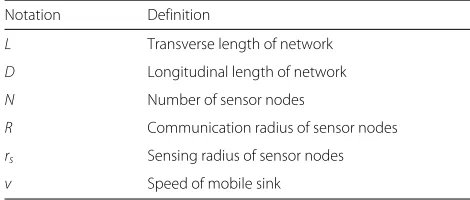
Table 1Notations and definitions
Notation Definition
L Transverse length of network
D Longitudinal length of network
N Number of sensor nodes
R Communication radius of sensor nodes
rs Sensing radius of sensor nodes
v Speed of mobile sink
(RCN) for each grid cell in step 2. To reduce the updat-ing range of a mobile sink’s location, we introduce the direction number (DN) in step 3.
1) Calculation of side length of grid cells
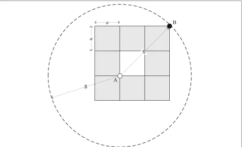
As illustrated in Fig. 2, each grid cell has up to eight neighbor grid cells, and the sensor nodes in neighbor grid cells are called the neighbor nodes. To enable nodes to communicate with the neighboring nodes, the relation of communication radiusRand a side length of grid cellsa need to satisfy Eq. (1). When the side length ais calcu-lated, mobile sink broadcasts some information in the net-work to establish the virtual structure. The information consists ofa,L, andD.
a≤
√
2R
4 (1)
2) Calculation of RCN of grid cells
After receiving the information broadcasted by a mobile sink, sensor nodes calculate the number of grid cells in both horizontal direction and vertical direction. The calculating process is defined by Eqs. (2) and (3).
nL=
L a
(2)
nD=
D
a
(3)
Based on the received information and their own coordi-nates, nodes can get an RCN, which indicates the location of a grid cell that the node belongs to; the calculating process is given in Eqs. (4) and (5).
Mr=
yi a
Zhuet al. EURASIP Journal on Wireless Communications and Networking (2018) 2018:134 Page 6 of 20
Fig. 2The relationship between communication radius and a side length of a grid cell. The distance betweenAandBisR, and it is easy to calculate the value ofa
Sensor nodes in the same grid cell have the same RCN value, and the RCN will not be modified. When RCN is calculated, the network is as shown in Fig.3.
3) Calculation DN of grid cells
Since the initial location of a mobile sink is in the grid cell center, sensor nodes can get the RCN of the grid cell center according to the information they received. The calculating process is shown in Eqs. (6) and (7).
After calculating the initial RCN of mobile sink, sensor nodes get the DN of grid cells that they belong to accord-ing to the relation of (Mr_sink,Mc_sink) and their own RCN
(Mr,Mc). The comparing process is given in Eq. (8).
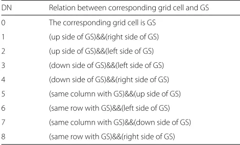
The grid cell where a mobile sink is located denoted the grid of sink (GS), and the relation between grid cell DN and GS is shown in Table2and Fig.4.
3.2.2 The election of head nodes in virtual grid cells
In our VGDCA-C, the virtual grid cell head nodes are to collect sensory data from the same grid cell, deliver sensory data, and maintaining the DN of the grid cell.
In the first election, all the sensor nodes broadcast their coordinates and RCNs, and the radius of broadcasting is
√
Fig. 3The RCN of virtual grid cell. It shows the RCS of virtual grid cell
After the operation of adding, sensor nodes sort their election lists. The election lists are sorted in ascending order by the abscissa, and if some sensor nodes have the same abscissas, the lists are sorted in ascending order by the ordinate. After the sorting operation, the sensor nodes in the same grid cell have the same election list. If a sensor node finds itself at the top of the election list, the sen-sor node broadcasts information of CellHead within the radius of√2a. The broadcasted CellHead consists of the indexes of sensor node in the election list. The other sen-sor nodes in the same grid cell receive the CellHead and
Table 2The relation between grid cells DN and GS
DN Relation between corresponding grid cell and GS
0 The corresponding grid cell is GS
1 (up side of GS)&&(right side of GS)
2 (up side of GS)&&(left side of GS)
3 (down side of GS)&&(left side of GS)
4 (down side of GS)&&(right side of GS)
5 (same column with GS)&&(up side of GS)
6 (same row with GS)&&(left side of GS)
7 (same column with GS)&&(down side of GS)
8 (same row with GS)&&(right side of GS)
mark sending node as a head node of that cell. Accord-ing to the sorted election list, the nodes in the grid are successively selected as the head nodes.
If some sensor nodes cannot broadcast CellHead, a wait-ing mechanism is introduced. If other nodes in the same grid cell cannot receive CellHead after a threshold period Thtime, the next sensor node in the election list tries to
broadcast CellHead .
3.2.3 The establishment of neighbor tables
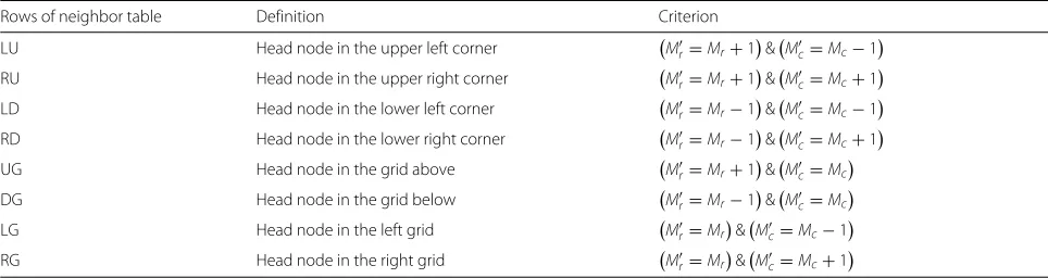
As each grid cell has up to eight neighbor grid cells, one head node has up to eight neighbor head nodes. In the process of establishing the neighbor tables, each head node broadcasts its coordinate and RCN in the commu-nication range. Meanwhile, each head node can receive information from other head nodes. Each head node
compares its RCN(Mr,Mc) with RCN of another head
nodeMr,Mc. According to the relation of(Mr,Mc)and
Mr,Mc, neighbor head nodes can be added to the corre-sponding rows of the neighbor table. The neighbor table
and corresponding criterion are shown in Table 3 and
Fig.5, respectively.
3.3 Data routing
Zhuet al. EURASIP Journal on Wireless Communications and Networking (2018) 2018:134 Page 8 of 20
Fig. 4The DN of virtual grid cell. The grid cell 0 is the cell wherein a mobile sink is located
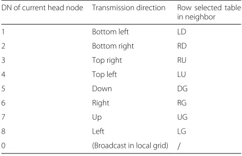
mobile sink. When source node has collected the sen-sory data, it encapsulates its RCN and sensen-sory data into a data packet and transmits it to the corresponding head node in the same grid cell, and the head node forwards the data packet to a neighbor head node according to the DN of the former. The data packet also includes other infor-mation, and the detail will be described in the following sections. The relation of the DN of head nodes and the corresponding transmission direction are shown in Fig.6 and Table4.
3.4 Trajectory planning of mobile sink
In our VGDCA-C, the moving region of a mobile sink is composed of a transverse moving belt and a longitudi-nal moving belt. The two moving belts are presented as a gray region in Fig.7. The two moving belts may switch to another column or row when target events change. Before the switching of a moving belt, the mobile sink will com-plete Numcyclemoving cycles in the moving belt. In Fig.7,
the grid cells in the gray region are called the moving belt grids. In one moving cycle, the mobile sink parks in
Table 3The neighbor table and corresponding criterion
Rows of neighbor table Definition Criterion
LU Head node in the upper left corner Mr=Mr+1&Mc=Mc−1
RU Head node in the upper right corner Mr=Mr+1
&Mc=Mc+1
LD Head node in the lower left corner Mr=Mr−1
&Mc=Mc−1
RD Head node in the lower right corner Mr=Mr−1
&Mc=Mc+1
UG Head node in the grid above Mr=Mr+1&Mc=Mc
DG Head node in the grid below Mr=Mr−1&Mc=Mc
LG Head node in the left grid Mr=Mr&Mc=Mc−1
Fig. 5The neighbor grid cells and corresponding rows in neighbor table. NodeAis the head node
different moving belt grids for different durations accord-ing to the collected sensory data. The mobile sink assigns weight values to the moving belt grids, and the weight val-ues affect the parking time of a mobile sink. When the mobile sink completes Numcyclemoving cycles in the
cur-rent moving belts, it estimates the location of the event region. Subsequently, the moving belts switch according to the corresponding strategy.
Fig. 6The DN of current head node and corresponding transmission direction. NodeAis the current head node, and the others are neighbor head nodes
Table 4The rules of selecting next hop head node
DN of current head node Transmission direction Row selected table in neighbor
1 Bottom left LD
2 Bottom right RD
3 Top right RU
4 Top left LU
5 Down DG
6 Right RG
7 Up UG
8 Left LG
0 (Broadcast in local grid) /
3.4.1 Trajectory of mobile sink in moving cycle
In our target application scenarios, the event region appears randomly. To adapt to this kind of application sce-narios, we design a “cross” moving trajectory for a mobile sink. As illustrated in Fig.7, the grid cell intersected by two moving belts is called the intersecting grid (IG). In one moving cycle, the mobile sink starts from IG and moves toward the direction whose DN is 5. After the mobile sink arrives at the grid cell whoseMris(nD−1),
it starts to move in the opposite direction. The mobile sink can move back to the IG, and then, the moving direc-tion switches to the direcdirec-tion whose DN is 8. When the mobile sink arrives at the grid cell whoseMcis(nL−1),
the mobile sink switches the moving direction to the opposite direction. The mobile sink moves in the direc-tion whose DN is 7 after moving back to the IG. When the mobile sink arrives at the grid cell whoseMr is 2, it
starts to move toward the IG again. After moving back to the IG, the mobile sink starts to move to the direction whose DN is 6 until it reaches the grid cell whoseMcis
2, then the mobile sink starts to move to the IG. When the mobile sink arrives at the IG, one moving cycle is completed.
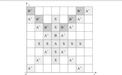
3.4.2 Calculation of weight value for moving belt grids
According to Section3.3, all the sensory data are routed to the moving belts. Different moving belt grids are respon-sible for different areas. As illustrated in Fig. 8, grid A has 13 responsible grid cells and grid B is responsi-ble for 6 grid cells. Hence, different moving belts grids have different workloads. When a mobile sink starts the first moving cycle in the current moving belts, it calcu-lates the weight value for each moving belt grid. Here,
W is used to represent the weight value. The RCN of
IG is(Mr_IG,Mc_IG), and the RCN of moving belt grid
Zhuet al. EURASIP Journal on Wireless Communications and Networking (2018) 2018:134 Page 10 of 20
Fig. 7The moving region of mobile sink in a moving cycle. The dashed line with arrow is the trajectory of sink
3.4.3 Allocation of parking time for mobile sink in the first moving cycle
Fig. 8The moving belt grids and corresponding responsible areas.S,A, andBare the moving regions of mobile sink in one moving cycle.A represents the region which gridAis responsible for andBrepresents the region which gridBis responsible for
sink is calculated by Eq. (14). We assume that in a mov-ing cycle, the parkmov-ing timetpais equal to the moving time tmoving_sink. Therefore, the total time of a moving cycle is
calculated by Eq. (15).
tmoving_sink=
2×a×(nL+nD−6)
v (14)
T =tmoving_sink+tpa=
4×a×(nL+nD−6)
v (15)
We allocatetpato each moving belt grid according to the
corresponding weight values, and the allocated time is the corresponding parking time. Thus, we need to get the sum of weight values, which is defined in Eq. (16).
Wall= nD−1
i=2
Wi,Mc_IG
+
nL−1
j=2
WMr_IG,j
−WMr_IG,Mc_IG
(16)
In the allocation process, the moving belt grids need to be classified into three categories. The first category is a top grid, and it refers to the moving belt grids that are adjacent to the boundary grids. The second category is IG, and the third category consists of other moving belt grids. The reason for grids classification is that the
num-ber of parking in different types of grid cells is different in a moving cycle. If a grid cell is a top grid, a mobile sink can park in this grid cell only once. We assume that the RCN of a moving belt grid is i,j. The number of times the mobile sink parks in different types of moving belt grids is calculated as follows:
• If a gridi,jis a top grid, then:
tp=
Wi,j Wall ×
tpa (17)
• If a gridi,jis IG, then:
tp
i,j=
W(i,j) Wall ×tpa
4 (18)
• If a gridi,jis the other moving belt grids, then
tp
i,j=
W(i,j) Wall ×tpa
2 (19)
Zhuet al. EURASIP Journal on Wireless Communications and Networking (2018) 2018:134 Page 12 of 20
parking time given above. When a mobile sink collects the sensory data, it counts the sensory data in the cor-responding counters. Therefore, in the following, we will talk about the counters in the mobile sink.
3.4.4 Counters of mobile sink
In the process of sensory data routing to the mobile sink, the sensory data carry the information on source nodes and routing. According to that information, the mobile sink counts the corresponding counters. When the sensory data are sensed, the source nodes attach their RCNs to the sensory data. When the sensory data are routed to the moving belt grid for the first time, then RCN of this moving belt grid is attached to the sensory data. The counters the mobile sink has are as follows:
• Cgm
i,j: In the sensory data, if the RCN of a moving belt grid that is first met isi,j, then the amount of sensory data is added to this counter.
• Cgm
i,j: This counter is used to record the number of the moving belt grids which the sensory data pass and the amount of sensory data are added to the counters corresponding to these passed moving belt grids.
• Chorizontal(i): The value ofi is from 1 to 3. As the
RCN of the source node is in the sensory data,Mrof
the source node can be obtained. IfMrof the source
node is larger than IGs, the value ofi is 1, and the amount of sensory data is added toChorizontal(1). If Mrof the source node is equal to IGs, the value ofi is
2. The value ofi is 3 when theMrof the source node
is smaller than IGs.
• Cvertical(i): The value ofi is from 1 to 3. As the RCN
of the source node is in the sensory data,Mcof the
source node can be obtained. IfMcof the source
node is larger than IGs, the value ofi is 1 and the amount of sensory data is added toCvertical(1). IfMc
of the source node is equal to IGs, the value ofi is 2. The value ofi is 3 when theMcof the source node is
smaller than IGs.
3.4.5 Dynamic adjustment of parking time
After completing the first moving cycle and moving back to the IG, a mobile sink readjusts the parking time for the next moving cycle according to its counters. Due to that, different grid cells handle different amounts of sensory data in the moving belts, so the mobile sink needs to park longer in the moving belt grid, which handles more sen-sory data. We divide the time of a moving cycle into two parts on average, of which is allocated byCgm
i,j, and another is allocated byCgr
When the recalculated parking time is discussed, the moving belt grids need to be classified into three cate-gories: top grids, IG, and other moving belt grids. We assume that the RCN of a moving belt grid is i,j. The time that mobile sink parking in different types of mov-ing belt grids is calculated as follows (the calculated time is the time of one parking in the grid):
• When a gridi,jis a top grid the time is defined by time is defined by
tpi,j=
parking. Before the start of a new moving cycle, all the counters of a mobile sink are set to zero. After the mobile sink completes Numcycle moving cycles, it
esti-mates the location of the event area according to the counters. The moving belt then moves toward the event area.
3.4.6 Moving trajectory of moving belts
As the source nodes are distributed centrally, the mobile sink needs to move toward the event area as close as possible such that the total length of the sensory data transmission is reduced and the energy consump-tion is decreased. Before the moving belts switch to another column or row, the mobile sink first com-pares Chorizontal(1), Chorizontal(2), and Chorizontal(3). If Chorizontal(1) has the largest value, the transverse
mov-ing belt switches to a neighbor row above. IfChorizontal(3)
has the largest value, the transverse moving belt switches to a neighbor row below. If Chorizontal(2) is the largest,
or two of three counters are equal, or all three coun-ters are equal, the transverse moving belt does not switch to another row. Similarly, the mobile sink compares Cvertical(1), Cvertical(2) andCvertical (3). IfCvertical(1) has
the largest value, the longitudinal moving belt switches to a neighbor column on the right. If Cvertical(3) is
the largest, the longitudinal moving belt switches to a neighbor column on the left. In other cases, the lon-gitudinal moving belt does not switch. According to this strategy, the mobile sink can get closer to the event area.
3.5 Local updating of mobile sink
When a mobile sink moves from one grid cell to another, the DN of grid cells needs to be updated to main-tain a reliable data routing. According to Section 3.3, the sensory data are routed to the mobile sink accord-ing to DN of grid cells. Hence, the updataccord-ing of DN of grid cells denotes the updating of the location infor-mation of a mobile sink. For further discussion, the updating operations need to be classified into two categories.
The first category refers to the situation that the mov-ing belts do not switch. In this situation, DNs of two grid cells need to be updated when the mobile sink enter into a new grid cell. The first grid cell is the one that the mobile sink is located in before entering the new one. The second grid cell is the one that the mobile sink entered, and this grid cell sets its DN to 0. The former grid cell sets its DN according to the moving direction. If mobile sink moves toward the direction whose DN is 5, the DN of the former grid cell is set to 7. If the direction DN is 8, the former’s DN is set to 6. If the direction has DN is 7, the former’s DN is set to 5. If the direction DN is 6, the former’s DN is set to 8.
The second category refers to the situation that the moving belts switch to another column or row. When a transverse moving belt switches to another row, both pre-vious row and current row need to update their DNs. When a longitudinal moving belt switches to another col-umn, both previous column and current column need to update their DNs. The updating is relevant to the grid cell where the mobile sink is located before moving. The relationship of grid cell DN and GS is shown in Fig. 4. Namely, when mobile sink updates a grid cell’s DN, it only needs to update the head node of the grid cell. Thus, the local updating not only reduces the update area but also reduces the number of the updated sensor nodes.
3.6 Re-election of head nodes
To prolong the network lifetime and balance the energy consumption of sensor nodes in each grid cell, the head nodes need to be regularly re-elected. First, the ratio of the residual energy of the current head node and its energy when it was elected is calculated. If that ratio is below a threshold Th, the head node broadcastsRe-Electionto start re-election of the corresponding grid cell. The Re-Electionincludes the ordinal number of the head nodes in the election listIndex. The sensor nodes in the same grid cell can receive the Re-Election and query the sen-sor node whose the ordinal number in the election list is (Index+1). If a sensor nodeAfinds that the sensor node queried itself, the sensor nodeAsends CellHead_01 to the current head node. After receiving CellHead_01, the cur-rent head node sends its neighbor list to the sensor node A. When sensor nodeAreceives the neighbor list of the current head node, it broadcasts CellHead_02. When the other sensor nodes receive CellHead_02, the sensor node Abecomes the new head node of the current grid cell, and the previous head node is retired. According to Eq. (1), all eight neighbor head nodes can receive CellHead_02,
and the neighbor head nodes then add sensor nodeAto
their neighbor lists. Before the new head node is ready, the sensory data are also transmitted to the previous head node. When the other sensor nodes are waiting for Cell-Head_02, if the waiting time exceeds the threshold Thtime,
they query the sensor node whose the ordinal number is (Index+2). If the current head node is the last one on the election list, then the sensor nodes will query the first sensor node on the election list in the next election.
4 Results and discussion
4.1 Simulation model
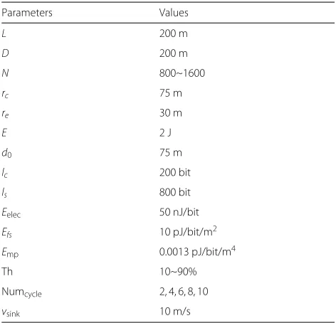
To evaluate the performance of our proposed algorithm, we designed the simulation experiment using the MAT-LAB platform. The simulation parameters are listed in
Table 5 and the values of the parameters are listed in
Table6. In our simulation, the target monitoring area was
Zhuet al. EURASIP Journal on Wireless Communications and Networking (2018) 2018:134 Page 14 of 20
Table 5Simulation parameters
Parameters Definition
L Transverse length of network
D Longitudinal length of network
N Number of sensor nodes
rc Communication radius of sensor nodes
re Radius of event area
E Initial energy of sensor node
d0 Threshold of communication
lc Size of control packet
ls Size of sensory data packet
Eelec Digital electronics
Efs Communication (d<d0)
Emp Communication (d≥d0)
Th Threshold of re-election
Numcycle Threshold of movig cycle
vsink Velocity of mobile sink
consisted ofNsensor nodes, and these sensor nodes had the same communication radiusrc and initial energyE.
The size of the control pocket was lc, and the size of
the sensory data packet was ls. We adopted the energy
model wherein if a sensor node receives nb bit sensory
data, the consumed energy is (nb×Eelec)J; if a sensor
node sendsnbbit sensory data, the consumed energy can
be classified into two categories. We assumed the trans-mission distance isd, and the threshold of transmission distance is d0. If d < d0, the consumed energy is
Table 6Values of simulation parameters
Parameters Values
Eelec 50 nJ/bit
Efs 10 pJ/bit/m2
Emp 0.0013 pJ/bit/m4
Th 10~90%
Numcycle 2, 4, 6, 8, 10
vsink 10 m/s
To simulate the centrally distributed event, we assumed event area is a circular area and all sensor nodes in this area are appointed as source nodes. The network lifetime was determined by the time when the first node runs out of its energy. In our VGDCA-C, the real-time data collection means that the source nodes upload sensory data immediately when the sensory data is sensed. In this context, we mainly focused on the balance of energy consumption to prolong the network lifetime. Thus, we focused on the lifetime performance and energy consumption balance, while the delay of sen-sory data transmission was not considered. We used the following aspects as performance metrics of simulation experiments:
• Network lifetime: defined by the time when the first node runs out of its energy
• Average residual energy: the mean value of residual energies of all the sensor nodes
• A variance of residual energy: the variance of residual energies of all the sensor nodes
• An average number of transmission hops: the mean value of transmission hops from a source node to the mobile sink.
4.2 Performance analysis under different system
parameters
In the simulation experiments of VGDCA-C, we first studied the impact of system parameters Th and Numcycle
on network performances, where Th denotes the thresh-old of the re-election of head nodes, which affects the equilibrium of energy consumption in a single grid cell, and Numcycleaffects the energy consumption in the entire
network and network lifetime. In these experiments, the number of sensor nodes was 1000, and the location of event area changed every 1000 s. The values of Th were 10, 30, 50, 70, and 90%, and the values of Numcyclewere 2,
4, 6, 8, and 10.
4.2.1 Network lifetime
Fig. 9The network lifetime under different system parameters (Th and Numcycle). When Th was 90% and Numcyclewas 8, the network lifetime could reach the maximum value
more balanced. We found that the network lifetime had the highest growth rate when Th varied between 70 and 90% because in that case, energy consumption within grid cell was the most balanced.
When we analyzed the situation from the vertical axis, we found that for the sameTh, network lifetime was
min-imal when Numcycle was 2. When Numcycle was 2, the
mobile sink needed to determine whether to switch the moving belts after every two completed moving cycles. According to the distribution of event area and the strat-egy of switching the moving belts, two moving belts switched in general circumstances. Hence, the grid cells of two rows and two columns needed to be updated. Therefore, much energy was consumed and network life-time was shortened. With the increase of Numcycle, the
network lifetime also increased. When Numcyclereached
8, the network lifetime had the maximum value because the updating operation did not consume much energy when the moving belts did not switch frequently. When Numcycle was 10, the network lifetime began to decrease
because all the sensory data were routed to the moving belts. If the moving belts were not switched for a long time, the sensor nodes in the moving belts could cause the “hot spot” problems, which would shorten the network lifetime. Thus, when Th was 90% and Numcyclewas 8, the
network lifetime could reach the maximum value.
4.2.2 Average residual energy
The average residual energy indicates the energy utiliza-tion rate of the network. As illustrated in Fig.10, with the increase of Th, the average residual energy decreased continuously. According to Fig. 9, the network lifetime
increase was caused by the increase of Th. Thus, the aver-age residual energy decreased. When Th was unchanged, the average residual energy was the lowest at Numcycleof
8, which means that the energy utilization rate was the best in that case. In Fig. 10, it can be seen that when Numcycle was equal to 2, the average residual energy was
lower than the average residual energy at Numcycle of 4.
However, when Numcyclewas 2, the network lifetime was
shorter than that when Numcyclewas 4. This is because the
moving belts needed to be constantly switched, and much energy was consumed to update the corresponding grid cells. Thus, the energy utilization rate was not high when Numcyclewas 2 because much energy was wasted. On the
other hand, when Numcycle was 8, the energy utilization
rate was the highest.
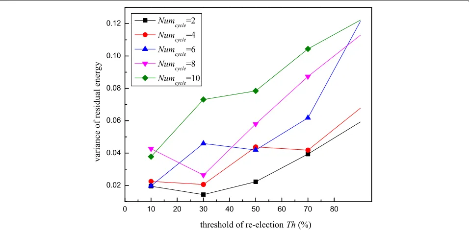
4.2.3 Variance of residual energy
The variance of residual energy indicates the balance of energy consumption. As illustrated in Fig.11, the variance was minimal at Th of 10% because only a small number of sensor nodes had consumed energy when the network ended. Most sensor nodes had almost the same residual energy. With the increase of Th, most sensor nodes began to consume energy, and the variance increased. When the Numcyclewas 2 and 4, the network lifetime was short, and
the variance was low. Although the energy consumption was balanced in that state, that was not an excellent sit-uation. When the Numcycle was 10, the variance reached
Zhuet al. EURASIP Journal on Wireless Communications and Networking (2018) 2018:134 Page 16 of 20
Fig. 10The average residual energy under different Th and Numcycle. When Numcycle was 8, the energy utilization rate was the highest
consumption of network was unbalanced. When Numcycle
was 6 and 8, the variance values were close, and the net-work had a better performance regarding the lifetime and average residual energy.
According to the analysis of network lifetime, aver-age residual energy, and residual energy’s variance, the network had the best performance at Th of 90% and
Numcycle of 8. There we set Th to 90% and Numcycle to
8 and compared the performance of the VGDCA-C and VGDD [27].
4.3 Comparison with VGDD
In this section, we compare the performance of the VGDCA-C and VGDD for different numbers of sensor
Fig. 12The comparison of VGDD and VGDCA-C in network lifetime. It shows that network lifetime of the VGDCA-C was longer that VGDD in our simulation model
nodes. The numbers of sensor nodes were 800, 1000, 1200, 1400, and 1600, respectively, and the time interval of event area change was 1000 s.
4.3.1 Network lifetime
As illustrated in Fig. 12, we compared the network life-time for different numbers of sensor nodes. With the increase of the number of sensor nodes, the network life-time of the VGDCA-C was always larger than that of the VGDDs. In the application scenarios with centrally
distributed events, the VGDCA-C could allocate parking time dynamically according to the counters of a mobile sink. The mobile sink would park longer time in the virtual grids with more sensory data. This method could reduce energy consumption and a total length of transmission. Meanwhile, two moving belts would switch dynamically according to the counters of a mobile sink. These counters indicated the location of event area, and the moving belts switched toward the event area. However, in the VGDD, a mobile sink moved by the predefined trajectory. When the
Zhuet al. EURASIP Journal on Wireless Communications and Networking (2018) 2018:134 Page 18 of 20
Fig. 14The comparison of VGDD and VGDCA-C in a variance of residual energy. The energy consumption balance of the VGDCA-C was slightly better than that of the VGDD
event area changed, the mobile sink of the VGDD could not adjust its trajectory to the event area. Hence, network lifetime of the VGDCA-C was longer. When the number of sensor nodes increased, the number of source nodes also increased. Moreover, there was no major fluctuation in the network lifetime due to the increase of the number of sensor nodes.
4.3.2 Average residual energy
As mentioned above, the average residual energy indicates the energy utilization ratio. As illustrated in Fig.13, with the increase of the number of sensor nodes, the average residual energy of the VGDCA-C was slightly lower than that of the VGDD, which indicates that energy utiliza-tion ratio of the VGDCA-C was higher than that of the
VGDD. In Fig. 12, it can be seen that network lifetime of the VGDCA-C was two times greater than that of the VGDD. However, the average residual energy of VGDCA-C was only slightly below than that of the VGDD, which indicates that the VGDCA-C could work longer when the same energy was consumed, which further means that the VGDCA-C had higher energy utilization ratio.
4.3.3 Variance of residual energy
As illustrated in Fig.14, when the number of sensor nodes was 800 and 1600, the variance value of the VGDCA-C was slightly larger than that of the VGDD. However, when the number of sensor nodes was 1000, 1200, and 1400, the variance value of the VGDCA-C was slightly lower than that of VGDD. The performances of two algorithms regarding the balance of energy consumption ware simi-lar. As the network lifetime of the VGDCA-C was larger than that of VGDD, the energy consumption balance of the VGDCA-C was slightly better than that of the VGDD.
4.3.4 Average number of transmission hops
As illustrated in Fig.15, when the number of sensor nodes varied from 800 to 1600, the average number of trans-mission hops was about 4 hops in the VGDCA-C. The corresponding number of the VGDD was greater than 7. The average number of transmission hops indicated that when the VGDCA-C was used, and source node sent data to the mobile sink, the hops of the packet could be reduced by 3 hops compared to the VGDD, which was because the trajectory of a mobile sink was adjusted dynamically and moved toward the event area. Meanwhile, when mobile sink allocated the parking time, the sink parked longer in the grids, which processed more sensory data. By con-stantly adjusting the movement trajectory and parking time, mobile sink could get closer to the source nodes, and the sensory data could be uploaded to the mobile sink faster. However, the mobile sink had a predeter-mined trajectory in the VGDD, so the mobile sink could not adjust its moving status according to the changes in the event area. Thus, the VGDCA-C had better real-time performance than the VGDD.
5 Conclusions
In this paper, the algorithm for real-time data collection for applications with centrally distributed events, called the VGDCA-C, is proposed and analyzed. Firstly, a vir-tual grid virvir-tual gird structure is introduced to initialize the network. The virtual grid structure can divide the network into several virtual square areas with the same size, where virtual grids of different areas have differ-ent RCN and DN. The structure is the basis of sensory data routing. Then, the routing of sensory data is dis-cussed. With the help of a virtual grid structure, the sensory data can be routed to the mobile sink easily
and automatically. Afterward, the trajectory planning of a mobile sink is proposed such that the mobile sink can move closer to the event area and park in the virtual grids longer, which increases the amount of sensory data. Using the proposed algorithm, the total length of rout-ing paths and the transmission delay are decreased. To reduce the energy consumption of updating of a mobile sink location, we propose the local updating. Finally, we proposed the re-election of head nodes in the virtual grid cells to balance energy consumption. Compared with the VGDD algorithm, the VGDCA-C algorithm prolongs network lifetime and decreases transmission delay in the applications with centrally distributed events.
Abbreviations
IWSNs: Industrial wireless sensor networks; VGDCA-C: Virtual grid-based real-time data collection algorithm for applications with centrally distributed events; MWST: Minimum Wiener index spanning tree; MST: Minimum spanning tree; RLW: Random line walk; EEGBDD: Energy efficient grid-based data dissemination routing mechanism; O-LEACH: Optimizing LEACH clustering algorithm; RNs: Convergence nodes; VGDRA: Virtual grid-based dynamic routes adjustment scheme; VGDD: Virtual grid-based data dissemination scheme; ID: Identification; RCN: Row column number; DN: Direction number; GS: Grid of sink; LU: Head node in the upper left corner; RU: Head node in the upper right corner; LD: Head node in the lower left corner; RD: Head node in the lower right corner; UG: Head node in the grid above; DG: Head node in the grid below; LG: Head node in the left grid; RG: Head node in the right grid; IG: Intersecting grid
Funding
The work is supported by “the Fundamental Research Funds for the Central Universities, no. 2017B14714”, supported by “the National Natural Science Foundation of China under grant no. 61572172”, and supported by “Changzhou Sciences and Technology Program, no. CE-20165023 and no. CE20160014” and “six talent peaks project in Jiangsu Province, no. XYDXXJ-S-007”.
Availability of data and materials
The values of simulation parameters are listed in Table6.
Authors’ contributions
CZ, XL, GH, JJ-N, and SZ designed the study, performed the research, analyzed the data, and wrote the paper. All authors read and approved the final manuscript.
Authors’ information
Chuan Zhu received the Ph.D. degree from the Department of Computer Science, Northeastern University, Shenyang, China, in 2009. And in December 2017, he finished his work as a Postdoctoral Researcher with Hohai University. He is currently a Lecturer in the Department of Information and
Communication System, Hohai University, China. He has authored over ten papers in related international conferences and journals. His current research interests are sensor networks, cloud computing, and computer networks. Xiaohan Long is a Master degree candidate of the Department of Internet of things and its Application at Hohai University, China. His current research interests are wireless sensor networks, underwater wireless sensor networks, cloud computing, and Android security software development.
Zhuet al. EURASIP Journal on Wireless Communications and Networking (2018) 2018:134 Page 20 of 20
and security. Dr. Han has served as a Co-chair for more than 50 international conferences/workshops and as a Technical Program Committee member of more than 150 conferences. He had been awarded the ComManTel 2014, ComComAP 2014, Chinacom 2014, and Qshine 2016 Best Paper Awards. He is a member of IEEE and ACM.
Jinfang Jiang is currently a Lecturer in the Department of Information and Communication System at Hohai University, China. She received her Ph.D degree in Information and Communication Engineering from Hohai University, China, in 2015. Her current research interests are security and localization for sensor networks.
Sai Zhang received the Master degree from the Department of Information and Communication System at Hohai University, China, 2017. He has published 1 paper in related international conferences and journals. He is working at Huawei Technologies Co., Ltd. currently.
Competing interests
The authors declared that they have no competing interests.
Publisher’s Note
Springer Nature remains neutral with regard to jurisdictional claims in published maps and institutional affiliations.
Received: 11 January 2018 Accepted: 1 May 2018
References
1. L Shu, M Mukherjee, X Wu, Toxic gas boundary area detection in large-scale petrochemical plants with industrial wireless sensor networks. IEEE Commun. Mag.54, 22–28 (2016)
2. L Shu, M Mukherjee, X Xu, K Wang, X Wu, A survey on gas leakage source detection and boundary tracking with wireless sensor networks. IEEE Access.4, 1700–1715 (2016)
3. B Ahmed, B Walid, R Herve, Optimal WSN deployment models for air pollution monitoring. IEEE Trans. Wireless Commun.16, 2723–2735 (2017) 4. M Amjad, L Jaime, S Sandra, A secure and low-energy zone-based
wireless sensor networks routing protocol for pollution monitoring. Wireless Commun. Mobile Comput.16, 2869–2883 (2016) 5. V Carlos, D Yezid, Delay/disruption tolerant network-based message
forwarding for a river pollution monitoring wireless sensor network application. Sensors.16, 436–460 (2016)
6. CZ Zulkifli, HN Hassan, W Ismail, et al, Embedded RFID and wireless mesh sensor network materializing automated production line monitorin. ACTA Phys. Polonica A.128(B86-B89) (2015)
7. G Han, L Liu, S Chan, R Yu, Y Yang, HySense: a hybrid mobile
CrowdSensing framework for sensing opportunities compensation under dynamic coverage constraint. IEEE Commun. Mag.55, 93–99 (2017) 8. G Han, L Zhou, H Wang, W Zhang, S Chan, A source location protection
protocol based on dynamic routing in WSNs for social internet of things. Futur. Gener. Comput. Syst.82, 689–697 (2017)
9. X Tian, Y Zhu, K Chi, J Liu, D Zhang, Reliable and energy-efficient data forwarding in industrial wireless sensor networks. IEEE Syst. J.11, 1424–1434 (2015)
10. G Han, X Yang, L Liu, W Zhang, A joint energy replenishing and data collection algorithm in wireless rechargeable sensor networks. IEEE Internet Thing J. (2017)
11. E Lee, S Park, J Lee, Novel service protocol for supporting remote and mobile users in wireless sensor networks with multiple static sinks. Wireless Netw.17, 861–875 (2011)
12. S Jannu, P Janam, A grid based clustering and routing algorithm for solving hot spot problem in wireless sensor networks. Wireless Netw.22, 1901–1916 (2016)
13. C Zhu, G Han, H Zhang, A honeycomb structure based data gathering scheme with a mobile sink for wireless sensor networks. Peer-to-Peer Netw. Appl.10, 1–16 (2016)
14. C Zhu, S Zhang, G Han, A greedy scanning data collection strategy for large-scale wireless sensor networks with a mobile sink. Sensors.16, 1432–1459 (2016)
15. S Han, I Jeong, S Kang, Low latency and energy efficient routing tree for wireless sensor networks with multiple mobile sinks. J. Netw. Comput. Appl.36, 156–166 (2013)
16. K Shin, S Kim, Predictive routing for mobile sinks in wireless sensor networks: a milestone-based approach. J. Supercomput.62, 1519–1536 (2012)
17. G Shi, J Zheng, J Yang, Z Zhao, Double-blind data discovery using double cross for large-scale wireless sensor networks with mobile sinks. IEEE Trans. Vehicular Technol.61, 2294–2304 (2012)
18. P Singh, R Kumar, V Kumar, An energy efficient grid based data dissemination routing mechanism to mobile sinks in Wireless Sensor Network, International Conference on Issues and Challenges in Intelligent Computing Techniques, 401–409 (2014)
19. C Tunca, M Dönmez, S Isik, C Ersoy, Ring routing: an energy-efficient routing protocol for wireless sensor networks with a mobile sink. IEEE Trans. Mobile Comput.14, 1947–1960 (2015)
20. N Wang, Y Chiang, Power-aware data dissemination protocol for grid based wireless sensor networks with mobile sinks. IET Commun.5, 2684–2691 (2011)
21. S Mottaghi, M Zahabi, Optimizing LEACH clustering algorithm with mobile sink and rendezvous nodes, AEU-Int. J. Electron. Commun.69, 507–514 (2015)
22. C Konstantopoulos, G Pantziou, D Gavalas, et al, A rendezvous-based approach enabling energy-efficient sensory data collection with mobile sinks. IEEE Trans. Parallel Distributed Syst.23, 809–817 (2012)
23. A Khan, A Abdullah, M Razzaque, VGDRA: a virtual grid-based dynamic routes adjustment scheme for mobile sink-based wireless sensor networks. IEEE Sensors J.15, 526–534 (2015)
24. A Kinalis, S Nikoletseas, D Patroumpa, Biased sink mobility with adaptive stop times for low latency data collection in sensor networks. Inf. Fusion. 15, 56–63 (2009)
25. S Ghafoor, M Rehmani, S Cho, An efficient trajectory design for mobile sink in a wireless sensor network. Comput. Electr. Eng.40, 2089–2100 (2014) 26. G Yang, S Liu, X He, N Xiong, Adjustable trajectory design based on node
density for mobile sink in WSNs. Sensors.16, 2091–2114 (2016) 27. A Khan, A Abdullah, M Razzaque, VGDD: a virtual grid based data
dissemination scheme for wireless sensor networks with mobile sink. International J. Distributed Sensor Netw.11, 1–17 (2015)