FULL PAPER
The ARASE (ERG) magnetic field
investigation
Ayako Matsuoka
1*, Mariko Teramoto
2, Reiko Nomura
3, Masahito Nosé
4, Akiko Fujimoto
5, Yoshimasa Tanaka
6,
Manabu Shinohara
7, Tsutomu Nagatsuma
8, Kazuo Shiokawa
2, Yuki Obana
9, Yoshizumi Miyoshi
2, Makoto Mita
1,
Takeshi Takashima
1and Iku Shinohara
1Abstract
The fluxgate magnetometer for the Arase (ERG) spacecraft mission was built to investigate particle acceleration pro-cesses in the inner magnetosphere. Precise measurements of the field intensity and direction are essential in studying the motion of particles, the properties of waves interacting with the particles, and magnetic field variations induced by electric currents. By observing temporal field variations, we will more deeply understand magnetohydrodynamic and electromagnetic ion-cyclotron waves in the ultra-low-frequency range, which can cause production and loss of relativistic electrons and ring-current particles. The hardware and software designs of the Magnetic Field Experiment (MGF) were optimized to meet the requirements for studying these phenomena. The MGF makes measurements at a sampling rate of 256 vectors/s, and the data are averaged onboard to fit the telemetry budget. The magnetometer switches the dynamic range between ± 8000 and ± 60,000 nT, depending on the local magnetic field intensity. The experiment is calibrated by preflight tests and through analysis of in-orbit data. MGF data are edited into files with a common data file format, archived on a data server, and made available to the science community. Magnetic field observation by the MGF will significantly improve our knowledge of the growth and decay of radiation belts and ring currents, as well as the dynamics of geospace storms.
Keywords: EMIC wave, Geospace, Magnetic field, Magnetometer, Radiation belts, Ring current, ULF wave
© The Author(s) 2018. This article is distributed under the terms of the Creative Commons Attribution 4.0 International License (http://creativecommons.org/licenses/by/4.0/), which permits unrestricted use, distribution, and reproduction in any medium, provided you give appropriate credit to the original author(s) and the source, provide a link to the Creative Commons license, and indicate if changes were made.
Introduction
The Arase (also known as Exploration of energization and Radiation in Geospace, ERG) satellite was success-fully launched on December 20, 2016, from the Uchin-oura Space Center. The spacecraft has apogee and perigee altitudes of ~ 32,000 and ~440 km, respectively, and an inclination of 32°, allowing the spacecraft to spend a majority of its time in the radiation belts. The spacecraft has an orbital period of 570 min and is spin-stabilized with a spin period of ~8 s.
The primary objective of the Arase mission is to reveal the generation mechanisms of relativistic elec-trons in radiation belts (Miyoshi et al. 2013; Miyoshi
et al. 2017). Particles of various energies and waves of various frequencies are considered to be involved in the electron acceleration process in the inner magne-tosphere. The Arase spacecraft measures the fluxes of ions and electrons over a wide energy range and detects electric and magnetic field oscillations over a wide frequency range to gain insight into the interactions between particles of different energies and waves of dif-ferent frequencies.
The magnetic field is a fundamental quantity in space plasma studies. The behavior of charged particles is often examined in a coordinate system referenced to the direc-tion of the magnetic field. Moreover, temporal variadirec-tions in the magnetic field play an important role in the trans-port, acceleration, and deceleration process of charged particles. The Magnetic Field Experiment (MGF) for the Arase mission was developed to conduct precise meas-urements of the static magnetic field and low-frequency magnetic field variations.
Open Access
*Correspondence: matsuoka@isas.jaxa.jp
1 Institute of Space and Astronautical Science, Japan Aerospace Exploration Agency, 3-1-1, Yoshinodai, Chuo-ku, Sagamihara, Kanagawa 252-5210, Japan
In "Science objectives and requirements for MGF" sec-tion of this of paper, we describe the scientific objectives of the MGF and its requirements. In "Instrument design", "Performance of MGF", and "Spacecraft magnetic cleanli-ness" sections, we explain the instrument design, perfor-mance, and the magnetic cleanliness of the spacecraft, respectively. The compliance of the MGF to meet speci-fication is discussed in each section. In "Operation" and "In-orbit calibration" sections, we describe the in-orbit operation of MGF and data calibration based on preflight experiments and in-orbit data analysis, respectively. In "Data processing flow" section, we show the MGF data processing flow for the scientific studies.
Science objectives and requirements for MGF Background field strength and direction
In the region of geospace surveyed by Arase, the mag-netic field is dominated by the component originating from the earth’s interior; therefore, the field is well rep-resented by the International Geomagnetic Reference Field (IGRF) model. Meanwhile, global electric currents flowing in the magnetosphere cause deviations from the intrinsic field, and temporal variations in the elec-tric current in the magnetosphere produce temporal variations in the magnetic field configuration.
Cummings et al. (1968) first reported that during mag-netospheric substorms, a tailward-stretched magnetic field recovers rapidly to a dipolar configuration, a phenomenon known as dipolarization. Magnetic dipolarization has often been discussed in association with bursty bulk flow (BBF) in the magnetotail (e.g., Angelopoulos et al. 1992; Takada et al. 2006). According to previous studies, particle acceleration occurs during dipolarization, although the causal relation-ship between the particle and magnetic field behaviors and the physical process connecting them are still under study (Lui 1991; McPherron and Chu 2016). In the inner magneto-sphere, a change in the field configuration can induce particle acceleration (Delcourt 2002). Understanding the relationship between variation in the field configuration and the genera-tion of energetic particles is one of the major objectives of the Arase project.
Observing the pitch-angle distribution of charged par-ticles is essential in studying wave–particle interactions because an anisotropic distribution contains free energy to excite plasma waves. Accurate determination of the field direction is necessary to study the dependence of the particle characteristics on the pitch angle. By meas-uring the pitch-angle distribution of the particle flux, we may gain information on phenomena occurring at vary-ing distances from the spacecraft along the field line. For example, particle dissipation at low altitudes could pro-duce a loss cone distribution observed on the same field line in the equatorial region (e.g., Thorne et al. 2010).
Pc3–5 ultra‑low‑frequency waves
Low-frequency magnetic field variations observed in the inner magnetosphere are categorized according to frequency and waveform characteristics. Narrow-band waves having a period of several tens to a few 100 s are called Pc3–Pc5 ultra-low-frequency (ULF) waves. ULF waves have the potential to energize particles (Elkington et al. 1999; Liu et al. 1999; Shprits et al. 2008 and ref-erences therein). Charged particles in the inner mag-netosphere basically have stable trajectories around the earth to keep the third adiabatic invariant constant. Meanwhile, acceleration could occur if particles periodi-cally scattered by magnetic perturbations undergo radial diffusion.
Until the 1990s, most observations in the inner mag-netosphere were made at geosynchronous orbit. The first comprehensive studies of ULF waves inward of the geostationary orbit were made using observations by the Active Magnetospheric Particle Tracer Explorers (AMPTE)/Charge Composition Explorer (CCE) at 5–8 RE (RE is the radius of the earth) (Anderson et al. 1990; Anderson 1994). Ali et al. (2015) investigated ULF waves observed by the Combined Release and Radiation Effects Satellite (CRRES) at L = 4–6.5 and evaluated the radial
diffusion coefficient. The contribution of ULF waves to relativistic electron generation is still controversial; Su et al. (2015) concluded that radial diffusion plays a key role, whereas a substantial number of studies support gyroresonant electron–whistler mode wave interaction as the predominant process (Miyoshi et al. 2003; Horne et al. 2005a, b; Shprits et al. 2008; Reeves et al. 2013 and references therein).
Electromagnetic ion‑cyclotron waves
It is proposed that the ions having a strong anisotropic pitch-angle distribution excite electromagnetic ion-cyclotron (EMIC) waves in the Pc1–2 band (from 0.1 to several Hz).
The statistics of the EMIC wave intensity observed by AMPTE/CCE were given by Anderson et al. (1992a), and the spatial distribution was demonstrated by Anderson et al. (1992b). The spatial occurrence frequency was fur-ther studied by Min et al. (2012) using Time History of Events and Macroscale Interactions during Substorms (THEMIS) data and by Keika et al. (2013) using AMPTE/ CCE data.
showed an EMIC rising tone event observed by Akebono in the deep inner magnetosphere and suggested the pre-cipitation of relativistic electrons via EMIC waves.
Requirements for the MGF
Magnetic field data are necessary not only for the reasons mentioned above but also for almost all scientific studies by Arase.
To capture phenomena that Arase should encounter, we defined the following requirements for MGF capabil-ity and performance: temporal variation noise level lower than 80 pT/√Hz in the 0.1–10 Hz frequency range, field
intensity error lower than 5 nT, and field direction error lower than 1°. These requirements apply to observations at L > 2 (L in RE is the distance of the field line from the earth center at the magnetic equator). We designed and tested the MGF hardware, software, and spacecraft sys-tem to meet these criteria. Sensor noise is described in "MGF performance" section, spacecraft noise in " Space-craft magnetic cleanliness" section, and the conformity of the MGF to the second and third criteria in "In-orbit calibration" section.
Instrument design Overview
The MGF is a fluxgate magnetometer designed based on the magnetometer (MGF-I) developed for the Bepi-Colombo mission’s Mercury Magnetospheric Orbiter (MMO) (Baumjohann et al. 2006, 2010). The analog-type magnetometer follows the basic design adopted for many space missions (Gordon and Brown 1972; Fuku-nishi et al. 1990; Kokubun et al. 1994; Yamamoto and Matsuoka 1998; Tsunakawa et al. 2010). Nevertheless, some elements of the sensor and electronics were newly developed to withstand the harsh radiation environment
of Mercury (Matsuoka et al. 2013). These elements are appropriate for the Arase spacecraft, which is also exposed to severe radiation.
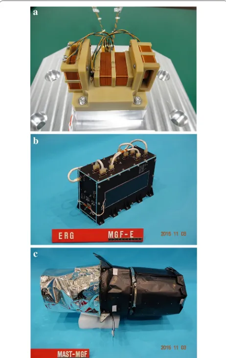
Figure 1 shows the overall configuration of the MGF. It consists of a sensor (MGF-S) and an electronics box (MGF-E). The MGF-E is installed inside the spacecraft body, on the −Z panel, where the −Z-direction roughly points toward the sun. It includes four electronics boards: the magnetometer circuit, the sensor temperature meas-urement circuit, the central processing unit (CPU), and the power supply unit (PSU). The PSU supplies ± 7 V power to the magnetometer circuit board and + 3.3 V to the CPU. Commands from the ground or issued auton-omously by the spacecraft system are transferred to the CPU from the mission data processor (MDP) by Space-wire protocol. The CPU exchanges the commands and data with the magnetometer circuit board by the Space-wire protocol as well. Two types of data are generated by the magnetometer circuit board: mission (magnetic field) data and housekeeping (HK) data. Mission and HK telemetry packets are created by the CPU and sent to the ground via the MDP. Meanwhile, ‘shared’ magnetic field data are distributed to other instruments onboard Arase. In parallel, near-real-time magnetic field data are com-piled with data from the extremely high-energy electron experiments (XEP) instrument and high-energy elec-tron experiments (HEP) instrument in space-weather telemetry packets, and downlinked immediately for near-real-time monitoring of the inner magnetosphere. The production/processing procedure of magnetic field data is described in "Onboard data processing" section.
The sensor (MGF-S) is mounted at the tip of an extend-able 5-m MAST. The cextend-ables connecting MGF-S with MGF-E are twist-pair with a shield, which is electrically connected to the spacecraft ground level.
Figure 2 shows photographs of the flight model MGF-S, MGF-E, and extendable MAST in stowed configuration.
Sensor (MGF‑S)
In the MGF-S unit, three sensor elements are mounted on the sensor base to measure the three orthogonal com-ponents of the magnetic field. A sensor element consists of a metal core, a driving coil, and a pickup/feedback coil. The core has an identical design to the 20-mm-diameter ring-shaped nickel–molybdenum Permalloy core for BepiColombo MMO MGF-IS. The driving coil is wound around the ring to excite the magnetic field in the core. The center axis of the pickup/feedback coil is along the diameter of the ring; this axis corresponds to the field measurement direction of the sensor element. A Pt tem-perature sensor is located on the back side of the sensor base. Temperature data are used to calibrate the mag-netic field data.
5‑m extendable MAST
The MGF sensor is mounted on the tip of the 5-m extend-able MAST to avoid magnetic interference from the space-craft. The MAST for Arase has nearly the same design as that for Nozomi (Yamamoto and Matsuoka 1998) and is similar to those used for Geotail (Kokubun et al. 1994), Kaguya (Tsunakawa et al. 2010), and BepiColombo MMO, except for the diameter, length, and material used. The MAST was in the stowed configuration at launch, and was deployed about 1 month after launch. Arase has two MAST units, one for the MGF sensor and the other for the search-coil sensor; these were deployed simultaneously in orbit to retain the dynamic balance of the spacecraft.
Circuit design
Figure 3 shows a block diagram of the MGF magnetic field measurement function. The sensor driver circuit excites an 11 kHz current in the drive coil wound around the sensor core. The signal amplitude detected by the sensor pickup coil at the second harmonic, 22 kHz, is propor-tional to the magnetic field. The 22 kHz component is selectively amplified by bandpass filters. The phase detec-tor outputs a voltage proportional to the amplitude of the 22 kHz component in the pickup signal. It is integrated and produces a feedback current to the pickup coil to can-cel out the external magnetic field at the sensor element. The feedback register defines the sensitivity, which is the ratio between the magnetic field and the output voltage of the integrator. Two feedback registers correspond to the two dynamic ranges, ± 8000 and ± 60,000 nT. A field-programmable gate array (FPGA) switches the feedback registers and controls synchronous timing of the phase detector according to commands sent from the ground.
When magnetic cancelation at the sensor is established, the output from the integrator represents the exter-nal magnetic field. The output is converted into a 20-bit digital signal by the analog-to-digital conversion (ADC) circuit, which consists of a delta-sigma modulator and a digital filter programed in the FPGA. The FPGA stores the filtered magnetic field (mission) data in a in first-out (FIFO) buffer with time stamps. Sensor temperature data are obtained from a different ADC in the tempera-ture measurement board. The FPGA transfers the mis-sion data stored in the FIFO buffer to the CPU, together with the HK data. The HK data include the sensor tem-perature, parameters used to operate the magnetometer board (synchronous timing for the phase detector and range information), and Spacewire connection status.
Performance of MGF Basic characteristics
Table 1 shows basic parameters representing the charac-teristics of the MGF. Two dynamic ranges, ± 8000 and
± 60,000 nT, are implemented for measurements at L > 2 and L < 2, respectively. The ADC is designed for a sam-pling rate of 256 vectors/s and digital resolution of 20 bits. The accuracies shown in the table are derived from ground calibration experiments, described in "Ground calibration" section.
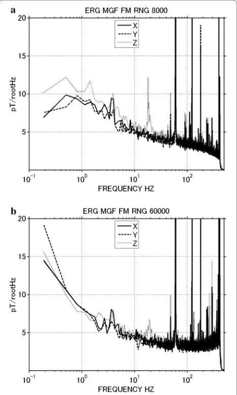
MGF performance
Figure 4 shows the noise spectrum of the analog output when the MGF-S sensor is placed in a magnetic shield-ing box. The peaks at 20, 50, and 60 Hz and higher har-monics are associated with environmental noise. Noise appearing at other frequencies is mostly attributed to the Barkhausen noise of the sensor. The properties of the noise are summarized in Table 2. In the dynamic range of ± 8000 nT, the typical noise intensity at 1 Hz is 9−10 pT/
√
Hz, and the root mean square (RMS) ampli-tude of the noise in the frequency band from 0.1–10 Hz is 35–40 pT. The noise generated in the ADC part was examined by investigating the digital output with sta-ble voltage supplied to the input. The RMS amplitude of Fig. 3 Block diagram of MGF magnetic field measurements
Table 1 Basic parameters of MGF for Arase (ERG)
Data sampling Dynamic range (nT) ± 8000 nT/± 60,000 nT Digital resolution (pT) 15/114 (20 bits) Original sampling
frequency (Hz) 256
Accuracy (RT) Sensitivity < 0.06% (± 8000 nT range)
< 0.10% (± 60,000 nT range)
Orthogonality (°) < 0.1 Accuracy (− 20 to
30 °C) Sensitivity change from RT 0.016% (range)± 8000 nT Offset (nT) < 2nT (± 8000 nT
range) Weight Sensor (g) 120
Electronics (g) 2780 Dimension Sensor (mm) 71 × 58 × 41H
Electronics (mm) 334 × 121 × 203H Power consumption + 3.3 V 932 mA (nominal)
+ 7 V 357 mA (nominal)
the output was about 2 least significant bits (LSBs) cor-responding to 31 pT, which is comparable to the noise generated by the analog part. These results satisfy the sensitivity requirement that the noise floor be lower than
80 pT/√Hz ("Requirements for the MGF" section).
Simi-larly, in the ± 60,000 nT range, the analog noise levels at 1 and 0.1–10 Hz RMS are 8−9 pT/
√
Hz and 32–34 pT, respectively. However, the resolution at the digital out-put is never better than the ADC noise intensity, 2 LSBs, which corresponds to 230 pT.
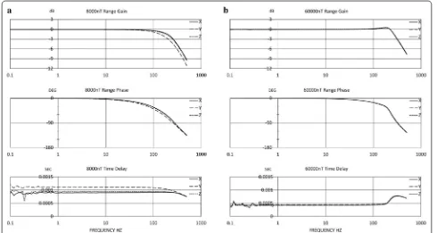
Figure 5 shows the response characteristics of the MGF analog part. The line plots show the integrator output (Fig. 3) for calibration signals applied to the sen-sor. The cutoff frequency (− 3 dB) is higher than 200 Hz for the ± 8000 nT range, and higher than 300 Hz for the
± 60,000 nT range. In the frequency range of 1–107 Hz
(107 Hz is the frequency nearest the cutoff of the ADC digital filter described later), phase delay at each fre-quency is determined with an accuracy better than 35 (20) μs for the ± 8000 (± 60,000) nT range. A summary of the test results is given in Table 2.
The overall frequency characteristics of the MGF are represented by a combination of the characteristics of the analog part, ADC, and subsequent averaging pro-cessing. Figure 6 shows the time domain window func-tion and the corresponding frequency response of the ADC, combined with the subsequent averaging pro-cessor. The ADC modulates the analog magnetic field data into delta-sigma 65 kHz signals. A finite impulse response (FIR) digital filter is applied to these signals, and 256 Hz samples are generated. The window length of the FIR filter is twice the sampling interval, 7.8 ms. The frequency response of the FIR filter, shown by a solid line in Fig. 6b, has a cutoff at 103.5 Hz, far below the cutoff frequencies of the analog signals. To reduce telemetry volume, the CPU averages the 256 Hz sam-ples down and resamsam-ples the data at a reduced rate. Figure 6b shows the response characteristics of the dig-ital filters for 128, 64, and 32 Hz sampling frequencies, with cutoff frequencies at 55, 28, and 14 Hz, respec-tively; these cutoff frequencies are far below those of analog signals. Because the time stamps are defined at the center of the data window, the FIR and averaging filters do not introduce any time delay. To summarize, MGF data are characterized by the frequency responses of the digital (FIR and averaging) filters and the time delay occurring in the analog circuit.
Ground calibration
Magnetic field sensitivity and sensor orthogonality were measured in the magnetic test facility at the Japan Aero-space Exploration Agency (JAXA) Tsukuba Space Center. The experimental details and results are discussed in Ter-amoto et al. (2017). Sensitivity was determined with an accuracy of 0.06% (± 8000 nT range) and the orthogonal-ity (angles between the measurement axes) with an accu-racy of 0.03° (Table 1).
Due to deformation of the sensor by temperature varia-tion, the sensitivity and offset depend on the sensor tem-perature. The sensitivity for various sensor temperatures was measured in the magnetic shielding room at JAXA’s Sagamihara Campus (Hirao et al. 1985). The increase in sensor sensitivity with temperature is caused by thermal expansion of the pickup/feedback coil dimensions. Sen-sitivity measurement error increased as the temperature decreased due to the difficulty in keeping the sensor tem-perature stable at low temtem-peratures. Nevertheless, in the temperature range from − 20 to 30 °C, the sensitivity variation from that at room temperature was determined Fig. 4 Noise spectrum of the analog output obtained when the
within 0.016%. This percentage is smaller than the deter-mination error of the absolute sensitivity, described above (0.06% for the ± 8000 nT range and 0.1% for the
± 60,000 nT range).
The measurement offset and its dependence on tem-perature were evaluated in the same experimental test. The offset variation was less than 2 nT for temperatures from − 20 to 30 °C (Teramoto et al. 2017), which meets the requirement of 5 nT ("Requirements for the MGF" section). However, we must note that spacecraft mag-netic cleanliness and sensor alignment, which contrib-ute to the magnetic field offset, have yet to be addressed; these are discussed below.
Spacecraft magnetic cleanliness
To achieve precise measurements of the magnetic field, reduction in magnetic interference from the spacecraft is important. Many efforts were made to optimize the magnetic cleanliness of the Arase spacecraft. The design of the installed components and spacecraft system were examined in view of magnetic cleanliness and modified to reduce interference as needed. The magnetic fields generated by individual components were measured to confirm the effectiveness of these efforts. In this sec-tion, we present the final evaluation results for magnetic cleanliness.
The stray field around the powered-off spacecraft was measured in the magnetic shielding chamber at JAXA’s Sagamihara Campus. Field vectors at 2.5-m distance from the center of the spacecraft were measured in 30° steps in elevation and 45° steps in azimuth. Figure 7a shows the measurement results, and Fig. 7b shows the superposition of the fields calculated by the measured magnetic moments of the individual components. The field intensity and its dependence on the azimuth were
similar for the superposition model (Fig. 7b) and post-assembly measurements (Fig. 7a). A comparison at elevation = 0° and azimuth = 0°, which is in the same direction from the spacecraft center as MAST deploy-ment, was most representative to check the validity of the model; measurement results indicated a field inten-sity of ~ 4 nT, whereas the model predicted ~ 3 nT. The difference is small; thus, the superposition model is considered to work well for evaluating the field around the spacecraft. The difference could be attributed to the properties of the magnetic materials used in the spacecraft, which would distort the magnetic field. The model indicates that the field intensity at the MGF-S position after MAST deployment is 0.18 nT, which is much smaller than the offset of the MGF instrument. Also, it is much lower than the required 5 nT described in "Requirements for the MGF" section.
Time-varying fields during system-level spacecraft function tests were also measured at the 2.5-m distance from the spacecraft center in the same magnetic shield-ing room. In this case, it was difficult to evaluate the noise from the spacecraft because the measured field was overwhelmed by noise believed to have originated from controllers located outside the shielding room. The noise appeared even when the spacecraft power was turned off, leading us to conclude that it must have radiated from cables connected to the controllers. For the possible worst-case scenario, in which noise from the spacecraft at the 2.5-m distance is comparable to the environ-mental noise, we estimated the noise to be lower than 100 pT/√Hz, except for a narrow-band enhancement at 7 Hz. If we assume that the noise decreases as the cube of the distance from the spacecraft center, it is estimated to be below 9 pT/√Hz at the MGF-S position after MAST deployment, which is comparable to the noise of the Table 2 Frequency characteristics of MGF
± 8000 nT range ± 60,000 nT range
MGF instrument itself, as shown in Fig. 5. Moreover, it is one order of magnitude below the required noise level (80 pT/√Hz) described in "Requirements for the MGF"
section.
From unit-level measurements and examinations of the magnetic noise prior to the system-level measurement, we determined that battery charging and the magnetic torquer generate time-varying magnetic noise over the required level. During the system-level spacecraft func-tion test in the shielding room, noise from the spacecraft exceeded the environmental noise when the battery was fast-charging and when the magnetic torquer was in operation. Field variation generated by the battery charg-ing current had an amplitude of ~ 6 nT at 2.5 m from the spacecraft center, corresponding to an amplitude of ~ 0.5 nT at the tip of the deployed MAST. Variation dur-ing torquer operation was about 70 times larger. There-fore, caution is warranted when using data acquired during fast battery charging after an eclipse and at all times when using data acquired during torquer opera-tion, which occurs at perigee in every orbital revolution.
Operation
Onboard data processing
As shown in Fig. 3, the mission and HK data from the MGF are transferred from the FPGA on the mag-netometer circuit board to the CPU by the Spacewire
protocol. The CPU board processes the mission and HK data; it also edits data packets that are transferred to the MDP. The data packets are transferred to the ground via the MDP and data management component (DMC) of the spacecraft system. In addition, the CPU generates near-real-time onboard shared data. These data are written into the shared data area in the relay packet and are then circulated among the scientific instruments and transferred to other instruments and the MDP.
Table 3 shows a list of magnetic field data produced by the MGF CPU. The MGF mission telemetry packet, which comprises magnetic field data and status infor-mation necessary for data processing on the ground, has five formats that are mutually exclusive. The check-out format contains all information in the mission data from the magnetometer circuit board. With the excep-tion of the checkout mode, the format differs with respect to the data sampling rate: 256 Hz (same as the original), 128, 64, or 32 Hz. The CPU software extracts valid data from the original magnetic field data trans-ferred from the magnetometer circuit board and aver-ages them according to the sampling rate.
second, this information is often made available only at a lower rate (nominally, once every 5 s) on the ground. Selected items in the HK data are compiled in spacecraft system HK packets and made available every second to ground control.
Onboard CPU software generates near-real-time and onboard shared data from the measured magnetic field data. Data are preliminarily calibrated based on the results of ground calibration experiments. Mag-netic field data at spin-time resolution are included in the Space Weather data packet and transferred to the ground immediately, where they are used as a near-real-time indicator of the inner magnetosphere’s condition. In contrast, shared MGF data, which have a cadence of 16 Hz, become instantaneously available to the CPUs of other science instruments and are used for onboard data processing.
Initial operation
The initial MGF operations were carried out from Janu-ary to March 2017, during which time, no science-quality data were produced. Table 4 shows the history of the operation. The initial checkout of the MGF was performed on January 10, and all functions of the MGF were confirmed to be normal. The MAST was deployed on January 17 without incident. Autonomous control of the dynamic range by the CPU software was initiated on February 8. The CPU software was updated on March 10 to accommodate regular observation.
Regular operation
MGF data have been acquired regularly since initiation on March 13, 2017. As of the time of the preparation of this manuscript (September 2017), the sampling rates of telemetry packet data are 256 Hz for L < 4 and 64 Hz for L > 4. These rates were selected to cover the proton cyclotron frequency, which is about 10 Hz at L = 4 and
decreases with increasing L. Fig. 6 a Window shape and b response characteristics of the digital
filter in the analog-to-digital convertor (ADC) and subsequent averag-ing processor for the MGF. The asterisks represent the Nyquist (half of the sampling) frequencies. The circles indicate the cutoff frequencies
For autonomous control of the dynamic range, the CPU software checks the peak field intensity from the three axis measurements during spacecraft rotation. To avoid unnecessary switching, the CPU changes the dynamic range only when the peak value exceeds a threshold for three successive rotations.
Figure 8 shows a plot of the magnetic field intensity measured by the MGF on March 28, 2017; the intensity results obtained using the IGRF model are included for comparison. The field intensity varied from ~ 100 nT at apogee to ~ 30,000 nT at perigee, with an orbital period of 9.5 h. As mentioned above, the sampling rate is 256 Hz for L < 4 and 64 Hz for the rest period. The dynamic range is ± 60,000 nT for about 1 h at perigee and ± 8000 nT
for the rest. On the logarithmic scale, the measured field intensity agrees well with the IGRF model when it is larger than 1000 nT; however, differences become more pronounced when the field is weak. This means that the
external field becomes more dominant as L increases. The difference is expected because this example was taken during the recovery phase of a storm driven by a co-rotating interaction region (CIR) in the solar wind.
Figure 9 shows an example of magnetic field meas-urement by the three sensor elements of the MGF. The X-axis is nearly along the MAST extension direction, the Z-axis is nearly parallel to the spacecraft Z-direction, and the Y-axis completes the right-hand coordinate. Because the spacecraft rotates about a spin axis aligned with the spacecraft’s Z-axis, MGF X and Y components show a sinusoidal wave form with a spin period of about 8 s. It is noteworthy that the Z-component shows a small-amplitude sinusoidal variation as well. Moreover, further inspection reveals that the amplitudes are slightly differ-ent between the X and Y components; this is caused by the inclination of the measurement directions of the sen-sor elements from the reference coordinates with respect to the spacecraft spin axis.
In‑orbit calibration
To precisely measure the magnetic field, we need to accu-rately evaluate sensor element alignments in the space-craft reference frame. Knowledge of the alignment is also necessary for accurate determination of the measure-ment offset.
The alignment is difficult to determine in ground experiments. Moreover, the alignment may change over time due to deformation of the MAST. The inclination angles can be calculated from the amplitude and phase of the sinusoidal wave forms in in-orbit data. Let us consider the simplest configuration when the directions of sensor elements X and Y perfectly coincide with the spacecraft X and Y directions, and the Z element directs to (sin γ cos φ, sin γ sin φ, cos γ) in the spacecraft ref-erence frame. The ratio of the time-varying waveform amplitudes between data of X/Y elements and those of Z element is sin γ. The phase difference between data of X element and those of Z element is φ. The relationship Table 3 MGF data produced by CPU
Data type Available on the
ground? Data rate B field resolution Coordinate Note
Mission Y 256 Hz 16 pT (± 8000 nT range)
Table 4 Major events of MGF in the initial operation period after launch
DATE in UT (month/day, 2017) Events
1/10 Initial checkout 1/17 MAST deployment
1/25 Test of CPU function to switch dynamic range autonomously 2/5 Test of CPU function for onboard
coarse calibration
Onboard shared data verification 2/8 Upload of preliminary parameters for
onboard coarse calibration Start autonomous switching of
dynamic range by CPU 2/17 Start MGF operation by timeline 3/7 Update parameters for onboard
coarse calibration
3/10 Update CPU software to adjust aver-aging process
becomes much more complicated when the inclinations of X and Y elements are considered. Figure 10 shows the relationship between non-orthogonal sensor coordinates and the spacecraft reference frame, as well as the defini-tion of misalignment angles α and β. We calculated the misalignment angles for every spacecraft rotation and took daily statistics of the results to determine α and β for the calibration.
Figure 11 shows the distributions of the sensor mis-alignment angles on March 19, 2017, the same day as Fig. 9. In the ± 8000 nT dynamic range, the distribu-tion of α (β) exhibited a clear peak at − 0.89° (− 0.91°) (Fig. 11a), and 73% (88%) of the α (β) samples were within
value of − 0.93° (− 0.30°). We note that the field inten-sity changes rapidly near the perigees, where the dynamic range is nominally ± 60,000 nT. Time variation of the
field intensity during a spin period could cause errors and broadening of the distribution of the calculated mis-alignment angle. The overall measurement accuracy of the magnetic field direction in inertial reference frames (geophysical coordinates) is determined by both the sensor alignment accuracy in the spacecraft reference frame and the angular accuracy of the spacecraft atti-tude determination. To date, we have yet to obtain full accuracy in spacecraft attitude. Therefore, the alignment accuracy in the inertial frame of reference is yet to be determined. However, if we assume a typical maximum error of the satellite attitude determination of 0.5°, the overall accuracy of the magnetic field direction is better than 1°, the requirement described in "Requirements for the MGF" section, for both the ± 8000 and ± 60,000 nT dynamic ranges. The accuracy for the ± 60,000 nT range is expected to be improved by an upgraded analysis approach that considers field intensity variation.
Measurement offsets of the magnetic field in the space-craft spin plane are evaluated using spacespace-craft rotation. The positive or negative shift values of the sinusoidal wave forms of the measured data are the summation of the artificial measurement offset and the spin-axis com-ponent of the natural field. The artificial measurement offsets are determined by separating these two, consid-ering the sensor alignment. The results are consistent with those from the ground calibration test (Teramoto et al. 2017); i.e., the in-flight data offset is dominated by the MGF instrumental offset. This is reasonable, as the magnetic offset generated by the spacecraft is negligible compared with the offset by the instrument, as described in "Spacecraft magnetic cleanliness" section. We will check this point by examining the consistency between measured and model (i.e., IGRF) fields.
Fig. 9 Example of magnetic field measurements by the three MGF sensor elements. Data are plotted for 60 s, starting at 00 UT on March 19, 2017. The X-axis is nearly along the MAST extension direction, the
Z-axis is nearly parallel to the spacecraft Z-direction, and the Y-axis completes the right-hand coordinate
Fig. 10 Relationship between sensor non-orthogonal coordinates and the spacecraft reference frame, as well as the definitions of the misalign-ment angles, α and β. a Angles of measurement directions in an orthogonal reference frame represented by ΦX, ΦY, ΦZ, ΘX, ΘY, and ΘZ are
deter-mined in the ground calibration. bO1 is defined as an orthogonal coordinate that has the same X-direction and coplanar X–Y with the sensor. c
Data processing flow
Arase telemetry data are stored in the Scientific Infor-mation Retrieval and Integrated Utilization System (SIRIUS) at the Institute of Space and Astronautical Sci-ence (ISAS)/JAXA. The MGF mission and HK telemetry packets are extracted from Arase telemetry data. The raw magnetic field data in the mission packets are converted into calibrated magnetic field vectors in the spacecraft reference frame using the calibration parameters.
As mentioned in "Operation" section, the sampling rate of the data in the MGF mission telemetry packet
is 256, 128, 64, or 32 Hz. Data are converted into the physical magnetic field vectors in the rotating spacecraft coordinates by calibration parameters, namely sensitiv-ity, offset, and alignment. Besides the product from the 128 Hz telemetry raw data, 128 Hz vector calibrated data are generated by averaging 256 Hz vector data. Similarly, 64 Hz vector data are generated by averaging 256 and 128 Hz vector data. The original and averaged vectors are despun into non-rotating spacecraft coordinates and geophysical coordinates. Spin averages are generated from the vectors in the non-rotating spacecraft coordi-nate and converted to vectors in the geophysical coor-dinates. The final products are archived as CDF files and made publicly available. The data are distributed by the ERG Science Center together with Space Physics Envi-ronment Data Analysis Software (SPEDAS) to handle the data. From March to August 2017, the sampling rate of the MGF mission telemetry data was either 256 or 64 Hz, which means that continuous data are available at 64 Hz and spin-period time resolutions.
Examples of in‑flight measurements
Figure 12 shows an example of MGF observation on March 27, 2017, made 1 day before the example taken during the main phase of the storm (Fig. 8). Large-ampli-tude ULF waves were observed, and it is clear that wave period changed over time. The wave period was ~ 60 s, and the waves exhibited Pc 3–4 characteristics in the first 30 min, corresponding to L = 4.9–5.5. Larger amplitude waves suddenly emerged at 18:25 and were present at L = 5.5–5.9. The period then became much longer, about 400 s, and the waves exhibited the characteristics of Pc 5 waves.
Figure 12 shows the excellent performance of the MGF in measuring ULF waves, which are major targets of the Arase mission. The wave event is presented here as a pre-liminary report. Detailed analyses of this and other simi-lar events will be published elsewhere.
Summary and conclusions
Tasks including system design, performance testing, ground calibration, and onboard software coding for the MGF instrument for Arase were completed with excellent results. MGF has been under normal scientific operation since March 2017. We have used data acquired in-orbit for precise sensor alignment and offset calibration.
The well-calibrated MGF data will significantly con-tribute to the scientific study of radiation belts and will improve our understanding of the mechanisms under-lying the production and loss of relativistic electrons. Fig. 11 Statistical results for the sensor misalignment angles α and β
on March 19, 2017. a In the ± 8000 nT dynamic range, the distribu-tion of α (β) has a peak at – 0.89° (– 0.91°), and 72.8% (87.7%) of the
Coordinated observation of the phenomena by multiple satellites, (e.g., the THEMIS mission, Van Allen Probes, and the Magnetospheric Multiscale (MMS) mission) and ground facilities should be promoted to further enhance the groundwork of our project (Fujimoto et al. 2012; Ter-amoto et al. 2016).
Abbreviations
ADC: Analog-to-digital converter; AMPTE/CCE: Active Magnetospheric Particle Tracer Explorers/Charge Composition Explorer; BBF: bursty bulk flow; CDF: Common Data Format; CIR: co-rotating interaction region; CPU: central processing unit; CRRES: Combined Release and Radiation Effects Satellite; DMC: data management component; EMIC: Electro-Magnetic Ion Cyclotron; ERG: Exploration of Energization and Radiation in Geospace; FIFO: in first-out; FIR: finite impulse response; FPGA: field-programmable gate array; GSM: Geocentric Solar Magnetospheric; HEP: high-energy electron experiments; HK: House Keeping; IGRF: International Geomagnetic Reference Field; ISAS: Institute of Space and Astronautical Science; ISEE: Institute for Space-Earth Environment Research; JAXA: Japan Aerospace Exploration Agency; LSB: least significant bit; MAST: extendable MAST; MDP: mission data processor; MGF: Magnetic Field Experiment; MGF-E: MGF electronic box; MGF-I: MGF Inboard (BepiColombo MMO); MGF-S: MGF sensor; MMO: Mercury Magnetospheric Orbiter; MMS: Magnetospheric Multiscale; PSU: power supply unit; RMS: root mean square; RT: room temperature; SIRIUS: Scientific Information Retrieval and Integrated Utilization System; SPEDAS: Space Physics Environment Data Analysis Software; THEMIS: Time History of Events and Macroscale Interac-tions during Substorms; ULF: ultra-low frequency; XEP: extremely high-energy electron experiments.
Authors’ contributions
AM is PI of Arase MGF. MT works for the MGF hardware test, final MGF data archive and analysis. RN works for the MGF hardware test and data analysis. MN works for the MGF data evaluation and analysis. AF works for the initial MGF planning, hardware design and data analysis. YT works for the MGF hardware development and data analysis. MS works for the MGF hardware development. TN works for the MGF data application to the space-weather forecasting. KS works for the coordination of studies by the MGF data and by ground facilities. YO works for the MGF data analysis. YM is the Arase project scientist. MM works for the EMC activities of the Arase spacecraft. TT is the Arase mission manager. IS is the Arase project manager. All authors read and approved the final manuscript.
Author details
Acknowledgements
The authors wish to express their sincere thanks to all of the ERG (Arase) project team members. We are also grateful for the manufacturers of MGF, Sumitomo Heavy Industries, Ltd., and Tierra Tecnica Corporation, as well as the manufacturer of the extendable MAST, NIPPI Corporation. The MGF calibration test was supported by the Environment Test Technology Unit of JAXA. The magnetic cleanliness activities were greatly supported by Dr. Mio Murashima. Ayako Matsuoka gratefully acknowledges valuable comments from Dr. Tateo Goka and Prof. Susumu Kokubun at MGF review meetings.
Competing interests
The authors declare that they have no competing interests.
Availability of data and materials
The ERG (Arase) MGF level-2 data will be available in the data server at the ERG Science Center operated by ISAS/JAXA and ISEE/Nagoya University. (http:// ergsc.isee.nagoya-u.ac.jp/).
Ethics approval and consent to participate Not applicable.
Funding
The Arase project is funded by ISAS/JAXA.
Publisher’s Note
Springer Nature remains neutral with regard to jurisdictional claims in pub-lished maps and institutional affiliations.
Received: 20 September 2017 Accepted: 7 February 2018
References
Ali AF, Elkington SR, Tu W, Ozeke LG, Chan AA, Friedel RHW (2015) Magnetic field power spectra and magnetic radial diffusion coefficients using CRRES magnetometer data. J Geophys Res Space Phys 120:973–995. https://doi.org/10.1002/2014JA020419
Anderson BJ (1994) An overview of spacecraft observations of 10 s to 600 s period magnetic pulsations in the earth’s magnetosphere. In: Engebret-son MJ, Takahashi K, Scholer M (eds) Solar wind sources of magne-tospheric ultra-low-frequency waves. American Geophysical Union, Washington, D.C., pp 25–43. https://doi.org/10.1029/gm081p0025 Anderson BJ, Engebretson MJ, Rounds SP, Zanetti LJ, Potemra TA (1990) A
sta-tistical study of Pc 3–5 pulsations observed by the AMPTE/CCE Magnetic Fields Experiment, 1. Occurrence distributions. J Geophys Res Space Phys 95:10495–10523. https://doi.org/10.1029/JA095iA07p10495
Anderson BJ, Erlandson RE, Zanetti LJ (1992a) A statistical study of Pc 1–2 mag-netic pulsations in the equatorial magnetosphere: 1. Equatorial occur-rence distributions. J Geophys Res Space Phys 97:3075–3088. https://doi. org/10.1029/91ja02706
Anderson BJ, Erlandson RE, Zanetti LJ (1992b) A statistical study of Pc 1–2 magnetic pulsations in the equatorial magnetosphere: 2. Wave properties. J Geophys Res Space Phys 97:3089–3101. https://doi. org/10.1029/91ja02697
Angelopoulos V et al (1992) Bursty bulk flows in the inner central plasma sheet. J Geophys Res Space Phys 97:4027–4039. https://doi. org/10.1029/91JA02701
Baumjohann W et al (2006) The magnetosphere of Mercury and its solar wind environment: open issues and scientific questions. Adv Space Res 38:604–609. https://doi.org/10.1016/j.asr.2005.05.117
Baumjohann W et al (2010) Magnetic field investigation of Mercury’s mag-netosphere and the inner heliosphere by MMO/MGF. Planet Space Sci 58:279–286. https://doi.org/10.1016/j.pss.2008.05.019
Cummings WD, Barfield JN, Coleman PJ (1968) Magnetospheric substorms observed at the synchronous orbit. J Geophys Res 73:6687–6698. https:// doi.org/10.1029/JA073i021p06687
Delcourt DC (2002) Particle acceleration by inductive electric fields in the inner magnetosphere. J Atmos Solar Terr Phys 64:551–559. https://doi. org/10.1016/S1364-6826(02)00012-3
Elkington SR, Hudson MK, Chan AA (1999) Acceleration of relativistic electrons via drift-resonant interaction with toroidal-mode Pc-5 ULF oscillations. Geophys Res Lett 26:3273–3276. https://doi.org/10.1029/1999GL003659 Fujimoto A, Miyoshi Y, Matsuoka A (2012) Science output from Pc 5 pulsation study by the ERG spacecraft. Trans Jpn Soc Aeronaut Space Sci Aerosp Technol Jpn 10:Tr_11–Tr_15. https://doi.org/10.2322/tastj.10.tr_11 Fukunishi H et al (1990) Magnetic field observations on the Akebono (EXOS-D)
satellite. J Geomagn Geoelectr 42:385–409. https://doi.org/10.5636/ jgg.42.385
Gordon D, Brown R (1972) Recent advances in fluxgate magnetometry. IEEE Trans Magn 8:76–82. https://doi.org/10.1109/TMAG.1972.1067268 Hirao K, Tsuruda K, Aoyama I, Saito T (1985) Large spherical magnetic shield
room. J Geomagn Geoelectr 37:581–588. https://doi.org/10.5636/ jgg.37.581
Horne RB, Thorne RM, Glauert SA, Albert JM, Meredith NP, Anderson RR (2005a) Timescale for radiation belt electron acceleration by whis-tler mode chorus waves. J Geophys Res Space Phys. https://doi. org/10.1029/2004ja010811
Horne RB, Thorne RM, Shprits YY, Meredith NP et al (2005b) Wave acceleration of electrons in the Van Allen radiation belts. Nature 437:227–230 Jordanova VK, Boonsiriseth A, Thorne RM, Dotan Y (2003) Ring current
asym-metry from global simulations using a high-resolution electric field model. J Geophys Res Space Phys. https://doi.org/10.1029/2003ja009993 Jordanova VK et al (2006) Kinetic simulations of ring current evolution during the Geospace Environment Modeling challenge events. J Geophys Res Space Phys. https://doi.org/10.1029/2006ja011644
Keika K, Takahashi K, Ukhorskiy AY, Miyoshi Y (2013) Global characteristics of electromagnetic ion cyclotron waves: occurrence rate and its storm dependence. J Geophys Res Space Phys 118:4135–4150. https://doi. org/10.1002/jgra.50385
Kersten T, Horne RB, Glauert SA, Meredith NP, Fraser BJ, Grew RS (2014) Elec-tron losses from the radiation belts caused by EMIC waves. J Geophys Res Space Phys 119:8820–8837. https://doi.org/10.1002/2014ja020366 Kokubun S, Yamamoto T, Acuna MH, Hayashi K, Shiokawa K, Kawano H (1994)
The GEOTAIL magnetic field experiment. J Geomag Geoelectr 46:7–21 Liu WW, Rostoker G, Baker DN (1999) Internal acceleration of relativistic
electrons by large-amplitude ULF pulsations. J Geophys Res Space Phys 104:17391–17407. https://doi.org/10.1029/1999ja900168
Lui ATY (1991) A synthesis of magnetospheric substorm models. J Geophys Res Space Phys 96:1849–1856. https://doi.org/10.1029/90JA02430 Matsuoka A, Shinohara M, Tanaka Y, Fujimoto A, Iguchi K (2013) Development
of fluxgate magnetometers and applications to the space science mis-sions. In: Oyama K-I, Cheng CZ (eds) An introduction to space instrumen-tation. Terra Scientific Publishing Company, Tokyo, pp 217–225. https:// doi.org/10.5047/aisi.021
McPherron RL, Chu X (2016) Relation of the auroral substorm to the substorm current wedge. Geosci Lett 3:12. https://doi.org/10.1186/ s40562-016-0044-5
Min K, Lee J, Keika K, Li W (2012) Global distribution of EMIC waves derived from THEMIS observations. J Geophys Res Space Phys 117:A05219. https://doi.org/10.1029/2012ja017515
Miyoshi Y, Morioka A, Misawa H, Obara T, Nagai T, Kasahara Y (2003) Rebuilding process of the outer radiation belt during the 3 November 1993 mag-netic storm: NOAA and Exos-D observations. J Geophys Res Space Phys 108:SMP 3-1–SMP 3-15. https://doi.org/10.1029/2001ja007542 Miyoshi Y, Sakaguchi K, Shiokawa K, Evans D, Albert J, Connors M, Jordanova
V (2008) Precipitation of radiation belt electrons by EMIC waves, observed from ground and space. Geophys Res Lett. https://doi. org/10.1029/2008gl035727
Miyoshi Y et al (2013) The energization and radiation in geospace (ERG) project. In: Summers D, Mann IR, Baker DN, Schulz M (eds) Dynam-ics of the earth’s radiation belts and inner magnetosphere. Ameri-can Geophysical Union, Washington, D.C., pp 103–116. https://doi. org/10.1029/2012gm001304
Nomura R, Shiokawa K, Sakaguchi K, Otsuka Y, Connors M (2012) Polarization of Pc1/EMIC waves and related proton auroras observed at subauroral lat-itudes. J Geophys Res Space Phys. https://doi.org/10.1029/2011ja017241 Nomura R et al (2016) Pulsating proton aurora caused by rising tone
Pc1 waves. J Geophys Res Space Phys 121:1608–1618. https://doi. org/10.1002/2015JA021681
Reeves GD et al (2013) Electron acceleration in the heart of the van allen radia-tion belts. Science 341:991–994. https://doi.org/10.1126/science.1237743 Sakaguchi K et al (2013) Akebono observations of EMIC waves in the slot
region of the radiation belts. Geophys Res Lett 40:5587–5591. https://doi. org/10.1002/2013gl058258
Shprits YY, Subbotin DA, Meredith NP, Elkington SR (2008) Review of modeling of losses and sources of relativistic electrons in the outer radiation belt II: local acceleration and loss. J Atmos Solar Terr Phys 70:1694–1713. https:// doi.org/10.1016/j.jastp.2008.06.014
Su Z et al. (2015) Ultra-low-frequency wave-driven diffusion of radia-tion belt relativistic electrons 6:10096. https://doi.org/10.1038/ ncomms10096. http://dharmasastra.live.cf.private.springer.com/articles/ ncomms10096#supplementary-information
Summers D, Thorne RM (2003) Relativistic electron pitch-angle scattering by electromagnetic ion cyclotron waves during geomagnetic storms. J Geophys Res Space Phys. https://doi.org/10.1029/2002ja009489
Takada T et al (2006) Do BBFs contribute to inner magnetosphere dipolariza-tions: concurrent cluster and double star observations. Geophys Res Lett. https://doi.org/10.1029/2006gl027440
Teramoto M, Nishitani N, Nishimura Y, Nagatsuma T (2016) Latitudinal depend-ence on the frequency of Pi2 pulsations near the plasmapause using THEMIS satellites and Asian-Oceanian SuperDARN radars. Earth Planets Space 68:22. https://doi.org/10.1186/s40623-016-0397-1
Teramoto M, Matsuoka A, Nomura R (2017) Ground calibration experiments of Magnetic field experiment on the ERG satellite (Japanese). JAXA Research and Development Memorandum JAXA-RM-16-003
Thorne RM, Ni B, Tao X, Horne RB, Meredith NP (2010) Scattering by chorus waves as the dominant cause of diffuse auroral precipitation. Nature 467:943–946
Tsunakawa H et al (2010) Lunar magnetic field observation and initial global mapping of lunar magnetic anomalies by MAP-LMAG onboard SELENE (Kaguya). Space Sci Rev 154:219–251. https://doi.org/10.1007/ s11214-010-9652-0