Communication efficient distributed weighted non linear least squares estimation

R E S E A R C H

Open Access

Communication efficient distributed

weighted non-linear least squares estimation

Anit Kumar Sahu

, Dusan Jakovetic

, Dragana Bajovic

and Soummya Kar

Abstract

The paper addresses design and analysis of communication-efficient distributed algorithms for solving weighted non-linear least squares problems in multi-agent networks.Communication efficiencyis highly relevant in modern applications like cyber-physical systems and the Internet of things, where a significant portion of the involved devices have energy constraints in terms of limited battery power. Furthermore,non-linear modelsarise frequently in such systems, e.g., with power grid state estimation. In this paper, we develop and analyze a non-linear

communication-efficient distributed algorithm dubbedCREDO−N L(non-linearCREDO).CREDO−N L generalizes the recently proposed linear methodCREDO(Communication efficient REcursive Distributed estimatOr) to non-linear models. We establish for a broad class of non-linear least squares problems and generic underlying multi-agent network topologiesCREDO−N L’s strong consistency. Furthermore, we demonstrate communication efficiency of the method, both theoretically and by simulation examples. For the former, we rigorously prove thatCREDO−N Lachieves significantly faster mean squared error rates in terms of the elapsed communication cost over existing alternatives. For the latter, the considered simulation experiments show

communication savings by at least an order of magnitude.

Keywords: Distributed estimation, Stochastic approximation, Statistical inference, Non-linear least squares

1 Introduction

We consider distributed non-linear least squares estima-tion in networked systems. The networked system con-sidered consists of heterogeneous networked entities or agents where the inter-agent collaboration conforms to a pre-assigned possibly sparse communication graph. The agents acquire their local, noisy, non-linear observations about the unknown phenomenon (unknown static vec-tor parameter θ) in a streaming fashion over discrete time instances t. The goal for each agent is to

contin-uously generate an estimate of θ over time instances t

in a recursive fashion, where the estimate update of an agent involves simultaneous assimilation of the newly acquired local observations, and the received information through messages with agents in its immediate neighbor-hood. The assumed setup is highly relevant in several emerging applications in the context of cyber-physical systems (CPS) and the Internet of things (IoT), like state

*Correspondence:[email protected]

2_{University of Novi Sad, Faculty of Sciences, Department of Mathematics and}

Informatics, 21000 Novi Sad, Serbia

Full list of author information is available at the end of the article

estimation in smart grid, predictive maintenance, and pro-duction monitoring in industrial manufacturing systems. For example, with continuous state estimation of a smart grid, the acquired measurements (voltages, angles) are in general non-linear functions of the unknown state; fur-ther, the measurements are inherently distributed across different physical locations (elements of the system), and they arrive continuously over time with a prescribed sam-pling rate. Furthermore, the scale (network size) of the distributed system (e.g., a large scale micro-grid) and near real-time requirements on the estimation results make distributed, fusion center-free processing a desirable choice.

An important aspect of distributed estimation algo-rithms in the context of the applications described above is communication efficiency, i.e., achieving good esti-mation performance with minimal communication cost. Real-world applications such as large-scale deployment of CPS or IoT typically involve entities or agents with lim-ited on board energy resources. In addition to the limlim-ited on board power, the energy requirement per unit com-munication is usually significantly higher than the energy

requirement per unit computation [48]. Hence, communi-cation efficiency is a highly desirable trait in such systems. Moreover, for large-scale systems which require continu-ous system monitoring, it is crucial to reduce the commu-nication cost as much as possible without compromising on the performance of the inference task at hand, which then ensure longer lifetime of such systems.

In this paper, we propose and analyze a communication efficient distributed estimator for non-linear observation

models that we refer to asCREDO−N L. The estimator

CREDO−N Lgeneralizes the recently proposed linear distributed estimatorCREDO, see [37,38], that is designed and works for linear measurement (observation) models only. Specific contributions of the paper are as follows.

We propose the non-linear distributed estimator

CREDO−N Lthat works for a broad class of non-linear observation models and where the model information in terms of the nodei’s sensing function and noise statistic is only available at the individual agentiitself. With the proposed algorithm, each agent communicates probabilis-tically sparsely over time. More precisely, the probability

which determines whether a node communicates at timet

decays sub-linearly to zero witht, which then makes the communication cost scale sub-linear with timet.

Despite dropping communications and the presence of non-linearities in the sensing model, we show that the proposed algorithm achieves the optimal O(1/t) rate of the mean square error (MSE) decay1. The achievability of the optimal MSE decay in terms of timettranslates into significant improvements in the rate at which MSE scales with respect to the per-agent average communication costCt up to time t, namely fromO(1/Ct)with existing

methods, e.g., [15,16,31,34–36,40], toO1/C_t2−ζwith the proposed method, whereζ >0 is arbitrarily small. We also establish strong consistency of the estimate sequence at each agent, showing that each agent’s local estimator converges almost surely to the true parameterθ. Simula-tion examples confirm significant communicaSimula-tion savings ofCREDO−N Lover existing alternatives, by at least an order of magnitude.

We now briefly review the literature on distributed

inference and motivate our algorithm CREDO−N L.

Distributed inference algorithms can be broadly divided into two classes based on the presence of a fusion center. The first class assumes presence of a fusion cen-ter, e.g., [11, 23, 26, 27, 47]. The fusion center assigns sub-tasks to the individual agents and subsequently fuses the information from different agents. However, when the data samples are geographically distributed across the individual agents and are streamed in time, fusion center-based solutions are impractical.

The second class of distributed inference methods is fusion center-free. These works typically assume that the

agents are interconnected over a generic network, and each agent acquires its local measurements in a streaming fashion. These estimators are iterative (recursive), where at each iteration (time instance), each agent assimilates its new measurement and exchanges messages with its immediate neighbors, see, e.g., [2, 4–6, 14, 20, 22, 24, 25, 28–31, 34–36, 39, 43, 46]. Most related to our work are references that consider distributed estimation under non-linear observation models, as we do here, or distributed convex stochastic optimization, e.g., [15, 16, 31, 34–36, 40]. However, among these works, the best achievedMSE communication rateisO(1/Ct). In contrast,

we establish here a strictly faster MSE communication rate equal to O

1/C_t2−ζ

(ζ > 0 is arbitrarily small). Finally, it is worth noting that there exist a few distributed algorithms (without fusion node) that are also designed to achieve communication efficiency, e.g., [13,21,44–46]. In [46], a data censoring method is employed to save in terms of computation and communication costs. How-ever, the communication savings in [46] is a constant proportion with respect to a vanilla method which uses all allowable communications at all times. In [21], the com-munication savings come at a cost of extra computations. References [13, 44, 45] also consider a different setup than we do here, namely they study distributed optimiza-tion (with no fusion center) where the data is available a priori (i.e., it is not streamed). In terms of the strat-egy to save communications, references [13, 21, 44, 45]

consider, respectively, deterministically increasingly

sparse communication, adaptive communication scheme, and selective activation of agents. These strategies are different from ours that utilizes a randomized, increasing, “sparsification” of communications.

Consensus+innovationsmethods, see, e.g., [16,17,19,20]), are a sub-class of distributed recursive algorithms (the second class of algorithms mentioned above) that process data in a streaming fashion. With consensus+innovation methods, each node updates its estimate at each itera-tion two-fold: by weight-averaging its soluitera-tion estimate (consensus) with the neighbors’ solution estimates and by assimilating its newly acquired data sample (inno-vation). Therein, the consensus and innovation weights are usually time-varying and are carefully designed towards achieving optimal asymptotic performance, mea-sured, e.g., through asymptotic covariance of the estimate sequence. Within the class ofconsensus+innovations dis-tributed estimation algorithms (see, e.g., [18, 20]), the design of communication efficient methods has been addressed in [37], see also [38], for linear observation models, wherein a mixed time-scale stochastic

approx-imation method dubbed CREDO has been proposed.

We extend here CREDO to non-linear observation

models. Technically speaking, establishing convergence

involves establishing guarantees for existence of stochastic Lyapunov functions for the estimate sequence. The update

of the estimate sequence in CREDO−N L involves a

gain matrix which is in turn a function of the estimate itself. Moreover, in addition to the gain matrix being a function of the estimate, the sensing functions exhibit localized behavior in terms of smoothness and global observability in the proposed algorithm. Hence, the setup considered in this paper requires technical tools different fromCREDO, which we develop in this paper.

The rest of the paper is organized as follows. Section2 describes the problem that we consider and gives the needed preliminaries on conventional (centralized) and distributed recursive estimation. Section 3 presents the

novel CREDO−N L algorithm that we propose, while

Section4states our main results on the algorithm’s perfor-mance. Section 5presents the simulations experiments, and finally, we conclude in Section7. Proofs of the main results are relegated to AppendixA.

2 Model and preliminaries

2.1 Sensing and network models

Letθ ∈ , where ⊂ RM (the properties of it to be

specified shortly) be anM-dimensional parameter that is to be estimated by a network ofN agents. Every agentn at time indextmakes a noisy observationyn(t), a noisy

function ofθ. Formally, the observation model for then-th agent is given by,

yn(t)=fn(θ)+γn(t), (1)

where fn : RM → RMn is a non-linear sensing

func-tion, whereMn M, {yn(t)} ∈ RMn is the observation

sequence for then-th agent and {γn(t)} is a zero mean

temporally independent and identically distributed (i.i.d.) noise sequence at then-th agent with nonsingular covari-anceRn, whereRn ∈ RMn×Mn. The noise processes are

independent across different agents. We state an assump-tion on the noise processes before proceeding further.

Throughout, we denote by·theL2-norm of its vector

or matrix argument and byE[ .] the expectation operator.

Assumption 1There exists1 > 0, such that, for all n, Eγn(t)2+1

<∞.

We remark that the main results of the paper (Theorems

4.1 and 4.2) continue to hold even if 1 = 02. The

above assumption encompasses a general class of noise distributions in the setup.

The heterogeneity of the setup is exhibited in terms of the agent dependent sensing functions and the noise covariances at the agents. Each agent is interested in

reconstructing the true underlying parameter θ. We

assume an agent is aware only of its local observation model, i.e, the non-linear sensing functionfn(·)and the

associated noise covarianceRn, and hence, it has no

infor-mation about the observation matrix and noise processes of other agents.

The agents are interconnected through a communica-tion network that we shall assume throughout the paper

is modeled as an undirected simple connected graph

G = (V,E), withV = [1· · ·N] andEdenoting the set of agents (nodes) and communication links, see [3]. (With

the proposedCREDO−N Lmethod, the available links

in E will be activated selectively across algorithm itera-tions in a probabilistic fashion, as it will be detailed in Section3). The neighborhood of nodenin graphGis

n= {l∈V|(n,l)∈E}. (2)

The node n has degree dn = |n|. The structure of

the graph is described by theN × N adjacency matrix,

A = A = [Anl],Anl = 1, if(n,l) ∈ E,Anl = 0,

other-wise. LetD = diag(d1· · ·dN). The graph LaplacianL= D−Ais positive semidefinite, with eigenvalues ordered as 0 = λ1(L) ≤ λ2(L) ≤ · · · ≤ λN(L). The

eigenvec-tor ofLcorresponding toλ1(L)is(1/ √

N)1N. (Here,1N

is theN-dimensional vector with all entries equal to one.) The multiplicity of its zero eigenvalue equals the number of connected components of the network; for a connected graph,λ2(L) >0. This second eigenvalue is the algebraic connectivity or the Fiedler value of the network (see [7] for instance).

Example: distributed static phase estimation in smart grids

Many applications within cyber physical systems and the Internet of things can be modeled as non-linear dis-tributed estimation problems of type (1). Such class of models arises, e.g., with state estimation in power sys-tems; therein, a phasorial representation of voltages and currents is usually utilized, wherein non-linearity in gen-eral emerges from power-flow equations [1,33]. Here, we focus on the specific problem within the class, namely distributed static phase estimation in smart grids. We describe the model briefly and refer to, e.g., [12, 19] for more details. Here, graphGcorresponds to a power grid network ofn= 1, ...,Ngenerators and loads (here, a sin-gle generator or a sinsin-gle load is a node in the graph), while the edge setEcorresponds to the set of transmission lines or interconnections. (For simplicity, even though not nec-essary, we assume that the physical interconnection net-work matches the inter-node communication netnet-work.)

Assume that G is connected. The state of a node n is

described by(Vn,φn), whereVnis the voltage magnitude

andφn is the phase angle. As commonly assumed, e.g.,

[12], we let the voltages Vn be known constants; on the

other hand, angles φn are unknown ant are to be

power flow across the transmission line between nodesn andlcan be expressed as, e.g., [12]:

Pnl(φ)=VnVlbnl sin(φnl), (3)

where φ is the vector that collects the unknown phase

angles φn across all nodes,bnl is line(n,l)’s admittance,

andφnl = φn−φl. Denote byEm ⊂ E the set of lines

equipped with power flow measuring devices. The power flow measurement at line(n,l)is then given by:

ynl(t)=Pnl(φ)+γnl(t)=VnVlbnlsin(φnl)+γnl(t), (4)

where{γnl(t)} is the zero mean i.i.d. measurement noise

with finite moment E[|γnl(t)|2+1], for some 1 > 0. Assume that each measurementynl(t)is assigned to one

of its incident nodesnorl. Further, let_ndenote the set of all indexeslsuch that measurementsy_nl(t)are available at noden. Then, it becomes clear that the angle estimation problem is a special case of model (1), with the measure-ment vectorsyn(t)=[ynl(t), l∈n] ,n=1, ...,N, noise

vectorsγn(t) =[γnl(t), l ∈ n] ,n= 1, ...,N, and

sens-ing functionsfn(φ) =[VnVlbnl sin(φnl), l ∈ n] .n =

1, ...,N. It can be shown that under reasonable assump-tions on phase angle ranges (that correspond to the

admis-sible parameter set ) and the smart grid network and

admittances structure, the assumptions we make on the

sensing model are satisfied,3and hence,CREDO−N L

can be effectively applied; we refer to [12,19] for details.

2.2 Preliminaries: centralized batch and recursive weighted non-linear least squares estimation

In this subsection, we go over the preliminaries of cen-tralized and distributed weighted non-linear least squares estimation.

Consider a networked setup with a hypothetical fusion center which has access to the samples collected at all nodes at all times. In such a setting, in lieu of the sensing model as described in (1), one of the classical algorithms that finds extensive use is the weighted non-linear least squares (WNLS) (see, for example, [15]). The applicability of WNLS to fairly generic setups which are character-ized by the absence of noise statistics makes it particularly appealing in practice. We discuss properties of the WNLS estimator before proceeding further. Define the cost func-tionQtas follows:

Qt(z)= t

s=0

N

n=1

(yn(s)−fn(z)) Rn−1(yn(s)−fn(z)).

(5)

The hypothetical fusion center in such a setting gen-erates the estimate sequence θt in the following way:

_θt∈argmin_z∈Qt(z). (6)

The consistency and the asymptotic behavior of the esti-mate sequence{θt} have been analyzed in the literature

under the following weak assumptions:

Assumption 2 The set is compact convex subset of RM _{with non-empty interior int() and the true (but} unknown) parameterθ ∈int().

Assumption 3The sensing model is globally observable, i.e., any pair θ,θ´ of possible parameter instances in satisfies

N

n=1

fn(θ)−fn

´

θ2=0 (7)

if and only ifθ = ´θ.

Assumption 4The sensing function fn(.) for each n is continuously differentiable in the interior int()of the set

. For eachθin the set, the (normalized) gain matrix _θ defined by

θ = 1

N N

n=1

∇fn(θ)Rn−1∇fn (θ), (8)

is invertible, where∇fn(·) ∈ RM×Mn denotes the gradient offn(·).

Smoothness conditions on the sensing functions, such

as the one imposed by Assumption 3, are common in

statistical estimation with non-linear observations mod-els. Note that the matrix _θ is well defined at the true value of the parameterθ asθ ∈ int()and the continu-ous differentiability of the sensing functions holds for all θ ∈int().

The asymptotic properties of the WNLS estimator in terms of consistency and asymptotic normality are char-acterized by the following classical result:

Proposition 1([15])Let the parameter setbe compact and the sensing function fn(·)be continuous onfor each n. LetGtbe an increasing sequence ofσ-algebras such that Gt = σ

yn(s) t_s−₌1₀

N

n=1

. Further, denote byθ the true

parameter to be estimated. Then, a WNLS estimator ofθ exists, i.e., there exists an{Gt}-adapted processθt such that

_θt∈argmin_z∈Qt(z), ∀t. (9)

Moreover, if the model is globally observable, i.e., Assumption3holds, the WNLS estimate sequenceθt is consistent, i.e.,

Pθ

lim

t→∞θt=θ

whereP_θ(·)denotes the probability operator. Additionally, if Assumption4holds, the parameter estimate sequence is asymptotically normal, i.e.,

√

t+1θt−θ=⇒D N(0,c), (11)

where

c=(N θ)−1, (12)

θ is as given by (8) and =⇒D refers to convergence in

distribution (weak convergence).

The centralized WNLS estimator above suffers from significant communication overhead due to the inher-ent access to data samples across all aginher-ents at all times. Moreover, the minimization in (6) requires batch process-ing due to the non-sequential nature of the minimiza-tion. Recursive centralized estimators utilizing stochastic approximation type approaches have been proposed in [9, 10, 32, 41, 42], which mitigate the batch processing through the development of sequential albeit centralized estimators. However, such recursive estimators still suf-fer from the enormous communication overhead as the fusion center requires access to the data samples across all agents at all times and the global model information in terms of the sensing functions and the noise statistics across agents.

2.3 Preliminaries: distributed WNLS

Sequential distributed recursive schemes conforming to the consensus + innovations (see for example, [19] and Eq. (16) ahead) type update, where the agents’ knowledge of the model is limited to themselves have been proposed in [16,40]. In [16], so as to achieve the optimal asymptotic covariance, the global model information is made avail-able through a carefully constructed gain matrix update, which adds additional computation complexity and com-munication cost. In contrast with [16,40] introduces the trade off in terms of sub-optimality of the asymptotic covariance while using local model information at individ-ual agents for evaluating the gain matrix and thus saving communication cost. However, both the aforementioned algorithms in [16, 40] have the number of communica-tion scales linearly with the number of per-node sampled observations {yn(t)}. This paper builds upon the ideas

of sequential distributed recursive schemes catering to non-linear observation models as proposed in [16, 40] to construct a communication efficient scheme without compromising on the performance in terms of the mean square error. That is, we aim to achieve the order opti-mal MSE decay rate of(1/t)(see, e.g., [9]) in terms of the number of per-node processed samples, while reduc-ing the(t)communication cost which is a characteristic of previous approaches.

Before proceeding further, we briefly summarize the estimator in [40] which is referred to as the benchmark estimator henceforth. The overall update rule at an agent ncorresponds to

xn(t+1)=xn(t)−βt

l∈n

(xn(t)−xl(t))

neighborhood consensus −αt(∇fn(xn(t)))R−n1(fn(xn(t))−yn(t))

local innovation

(13)

and

xn(t+1)=P[xn(t+1)] , (14)

where n is the communication neighborhood of agent

n (determined by the Laplacian L); ∇fn(·) is the

gradi-ent of fn; P[·] the projection operator corresponding

to projecting on; and{βt}and{αt}are consensus and

innovation weight sequences given by

βt=

β0

(t+1)δ1, αt= α0

t+1, (15)

whereα0,β0 >0, 0 < δ1 <1/2−1/(2+1)and1was

defined in Assumption 1. From the asymptotic

normal-ity in Theorem 2 in [40], it can be inferred that the MSE decays asO(1/t).

Communication efficiency

The communication costCtis defined as the expected

number of per-node communications up to iteration t.

Formally, the communication costCtis given by

Ct=E

_t−1

s=0

I{agent n transmits at s}

, (16)

where agentn is arbitrary (the expectation in (16) does not depend onn) andIArepresents the indicator of event A. The communication cost Ct for both the centralized

WNLS estimator (where all agents transmit their samples

yn(t)to the fusion center at all timest) and the distributed

estimators in [16,40] isCt = (t), where we note that

the iteration countt is equivalent to the number of per node samples collected till timet. Technically speaking,

the MSE decays asO

1

Ct

.

3 CREDO−N L: a communication efficient distributed WNLS estimator

In this section, we present theCREDO−N Lestimator.

it to drop communications increasingly often. Technically speaking, for each noden, at every timet, we introduce a binary random variableψn,t, where

ψn,t=

ρt with probabilityζt

0 else, (17)

where ψn,t’s are independent both across time and the

nodes, i.e., acrosstandn, respectively as well are indepen-dent from nodes’ observations in (1). The random variable ψn,t abstracts out the decision of the node n at time t

whether to participate in the neighborhood information exchange or not. We specifically takeρtandζtof the form

ρt= ₍ ρ0

With the above development in place, we define the ran-dom time-varying Laplacian L(t), where L(t) ∈ RN×N which abstracts the inter-node information exchange as follows:

The communication protocol (17)–(20) assumes that the neighboring nodes communicate only when the cor-responding communication link is bi-directional. How bi-directional communication links can be enforced in practice is discussed next. Let us first assume that there exists a dedicated reliable bi-directional communication link between any two neighboring nodes. Consider a link

between nodes n and l at time t. If ψn,t = 1, node

n participates in communication, and it turns on both

its transmitting and receiving antennas. If ψn,t = 0, it

switches off both its transmitting and receiving antennas. Suppose that ψn,t = 1, and consider two scenarios: (1)

ψl,t = 0 and (2)l,t = 1. Consider first the former case.

Since nodenlistens the dedicated channel to nodeland nodeldoes not transmit, nodenverifies that it does not receive the respective message from nodel(e.g., within a prescribed time window), and hence, it does not incorpo-rate nodel’s estimate in its update. Also, asl,t=0, node l does not include the estimate by noden, by algorithm construction. Next, consider the case l,t = 1. In this

case, nodenlistens the channel and receives the message by nodel, and thus, it incorporates nodel’s estimate in its update. Completely symmetrically, nodellistens the chan-nel from nodento nodel, receives the respective message, and includes noden’s estimate in its update. Overall, the preceding discussion explains how the symmetric com-munication protocol can be established. A very similar consideration can be derived if the links are unreliable

but still symmetric, in the sense that if the link from n tolis strong enough to support communication, then so is the link from l to n. Finally, if the physical links can fail in an asymmetric fashion, then the proposed algo-rithm (see ahead (26)–(28) cannot be implemented in its direct form. More precisely, asymmetric failing links yield the Laplacian matricesL(t)become non-symmetric. The algorithm (26)–(28) and the corresponding analysis need to change in such scenario. This lies outside the scope of this paper, but it corresponds to an interesting future research direction.

With the protocol described in (17)–(20), both the weight assigned to the links and the probability of the existence of a link decay over time. We next consider the first moment, the second moment, and the variance of the Laplacian entries for{i,j} ∈E:

For future reference, we also introduce the mean Lapla-cian matrix{L(t)}asL(t) = E[L(t)], andL(t) = L(t)− where.Fdenotes the Frobenius norm. Also, note that

L(t)2_F =

We next give an assumption on the connectivity of the inter-agent communication graph.

Assumption 5The inter-agent communication graph is connected on average, i.e., λ2(L) > 0, which implies λ2(L(t)) > 0, whereL(t)denotes the mean of the

Lapla-cian matrix L(t) and λ2(·) denotes the second smallest

eigenvalue.

Assumption 5 ensures consistent information flow

among the agent nodes. Technically speaking, the com-munication graph modeled here as a random undirected graph need not be connected at all times. It is to be noted that Assumption 3 ensures that L(t) is connected at all times asL(t) = βtL. We now state additional

assump-tion on the smoothness of the sensing funcassump-tions for the distributed setup.

Assumption 6For each n, the sensing functionfn(·)is Lipschitz continuous on, i.e., for each agent n, there exists a constant kn>0such that

fn(θ)−fn(θ) ≤knθ −θ, (25)

for allθ,θ ∈.

With the communication protocol established, we pro-pose an update, where every nodengenerates an estimate sequence{xn(t)}, wherexn(t)∈RMin the following way:

xn(t+1)=xn(t)−βt

l∈n

ψn,tψl,t(xn(t)−xl(t))

neighborhood consensus −αt(∇fn(xn(t)))R−n1(fn(xn(t))−yn(t))

local innovation

(26)

and

xn(t+1)=P[xn(t+1)] , (27)

where n denotes the neighborhood of node n with

respect to the network represented byL,αtis the

inno-vation gain sequence which is given byαt = α0/(t+1), α0>0, andP[·] the projection operator corresponding

to projecting on. The random variableψn,tdetermines

the activation state of a noden. By activation, we mean, if ψn,t = 0, then nodencan send and receive information

in its neighborhood at timet. However, whenψn,t = 0,

noden neither transmits nor receives information. The

link between nodenand nodelgets assigned a weight of ρ2

t if and only ifψn,t=0 andψl,t=0.

The update in (26) can be written in a compact manner as follows:

x(t+1)=x(t)−(L(t)⊗IM)x(t)

+αtG(x(t))R−1(y(t)−f(x(t))). (28)

Here,⊗denotes the Kronecker product,IMdenotes the M×Midentity matrix, and:

x(t) =

x1(t) · · ·xN(t)

y(t) =

y1(t) · · ·yN(t)

x(t) =

x1(t) · · ·xN(t)

f(x(t)) = f1(x1(t)) · · ·fN(xN(t))

R−1 = diag

R−₁1,· · ·,R−_N1

G(x(t)) = diag [∇f1(x1(t)),· · ·,∇fN(xN(t))] .

Remark 1The Laplacian sequence that plays a role in the analysis in this paper, takes the form L(t)=βtL+L(t), whereL(t)the residual Laplacian sequence does not scale withβt owing to the fact that the communication rate is chosen adaptively and thus makes the Laplacian matrix sequence not identically distributed.

We refer to the parameter estimate update in (26) and the projection in (27) in conjunction with the

random-ized communication protocol as theCREDO−N L

algo-rithm. We propose a condition on the sensing functions (standard in the literature of general recursive procedures) that guarantees the existence of stochastic Lyapunov func-tions and, hence, the convergence of the distributed esti-mation procedure.

Assumption 7The following aggregate strict mono-tonicity condition holds: there exists a constant c1>0such

that for each pairθ,θ´inwe have that

N

n=1

θ− ´θ ∇fn(θ)

R−_n1fn(θ)−fn(θ´)

≥c1θ− ´θ 2

.

(29)

The instrumental step in analyzing the convergence of the proposed algorithm is ensuring the existence of appropriate stochastic Lyapunov functions (see, for

example [16–20]) which is in turn guaranteed by

Assumption7.

Remark 2It is to be noted that the Assumptions 6–7 are only sufficient conditions. Moreover, the assumptions which play a key role in establishing the main results, i.e., Assumptions2, 1, 6, and 7 are required to hold only in the parameter setinstead of the entire spaceRM, which makes our algorithm to apply to very general non-linear sensing functions.

We consider a specific example to give more intu-ition about the assumptions in this paper. If the fn(·)’s

are linear, i.e., fn(θ) = Fnθ, where Fn is the sensing

equivalent toN_n=1F_nR−_n1Fnbeing full rank.4Under this

context, the monotonicity condition in Assumption 7

is trivially satisfied by the positive definiteness of the matrixN_n=1F_nR−_n1Fn. We formalize an assumption on

the innovation gain sequence{αt}before proceeding further.

Assumption 8We require thatα0satisfies

α0c1>1, (30)

where c1is defined in Assumption7andα0is the

innova-tion gain at t=0.

The communication cost per node for the proposed algorithm is given byCt= ts−=10ζs=

t(1+)/2, which in turn is strictly sub-linear as <1.

4 Main results

In this section, we present the main results of the

pro-posed algorithmCREDO−N L, while the proofs of the

main results are relegated to Section 7. The first result concerns with the consistency of the estimate sequence {xn(t)}.

Theorem 4.1Let Assumptions1–3and5–8hold. Con-sider the sequence {xn(t)} generated by algorithm (26)– (27) at each agent n, with the parameters set to ρt =

ρ0

(t+1)/2, ζt =

ζ0

(t+1)(1/2−/2),and αt = α0/(t +1), where ρ0,ζ0,α0are arbitrary positive numbers. Then, for each n,

we have

Pθ

lim

t→∞xn(t)=θ

=1. (31)

Theorem4.1verifies that the estimate sequence

gener-ated byCREDO−N Lat any agentnis strongly

consis-tent, i.e.,xn(t)→θ almost surely (a.s.) ast→ ∞. While

Assumption 4 is needed for asymptotic normality results as in Proposition 1, it is not necessary for Theorem 4.1 (nor Theorem4.2ahead) to hold.

We now state a main result of this paper which estab-lishes the MSE communication rate for the proposed

algorithmCREDO−N L.

Theorem 4.2Let the hypothesis of Theorem 4.1 hold. Then, we have, for each n,

Exn(t)−θ2

=O

1 t

. (32)

Furthermore, for each n, we have:

Exn(t)−θ2=O

C−+12

t

, (33)

where0< <1and is as defined in (18).

We make several remarks on Theorems4.1and4.2.

Remark 3 Note that in Theorem 4.2can be taken to be arbitrarily small. Hence,CREDO−N Lachieves MSE communication rate arbitrarily close to1/C_t2. This is a sig-nificant improvement over existing non-linear distributed consensus + innovations estimation methods, e.g.,[18,20]. They have O(t) communication cost up to time t and a MSE iteration-wise rate of O(1/t), hence achieving O(1/Ct) MSE communication rates. CREDO−N Lachieves the order-optimal O(1/t) MSE iteration-wise rate with a reduced communication cost, thus significantly improving the MSE communication rate.

Remark 4 Observe thatCREDO−N Lalgorithm, with

βt = β0(t + 1)−1 has communication cost of Ct =

t0.5(1+). From this, we can see that MSE as a function ofCtis given by MSE=O

C−2/(1+)

t

.

Of course, withβt that decays faster than1/t, commu-nication cost reduces further. However, it can be shown that in this case the algorithm no longer produces good estimates. Namely, from standard arguments in stochas-tic approximation, it can be shown that forβt = β0(t+ 1)−1−δ_{, withδ > 0,CREDO−N L’s estimate sequence}

may not converge toθ.

Remark 5 TheCREDO−N Lalgorithm builds on our prior work in[37,38,40], but establishing Theorems4.1– 4.2 incurs several technical challenges with respect to our past work. Namely, from a technical standpoint, the

that the differences of Theorem4.1with respect to works [37, 38]mainly arise from the fact that we consider here nonlinear observation models. Due to this difference, sev-eral terms that appear in MSE upper bounds are bounded in a technically different way—see the proof of Lemma A1 in AppendixA. Therein, we need to use the arguments like the non-expansiveness property of projections and Lips-chitz continuity of functionsfn, none of which is explicitly used in[37,38].

5 Simulation experiments

This section corroborates our theoretical findings through simulation examples and demonstrates the communica-tion efficiency ofCREDO−N L.

Specifically, we compare the proposed communication efficient distributed estimator,CREDO, with the

bench-mark distributed recursive estimator in (13) and the

diffusion algorithm as in [43]5, which both utilize all inter-neighbor communications at all times, i.e., they have a linear communication cost. The example demonstrates that the proposed communication efficient estimator has a similar MSE iteration-wise rate as the two benchmark estimators. The simulation also shows that the proposed

estimator improves the MSE communication rate with

respect to the two benchmarks.

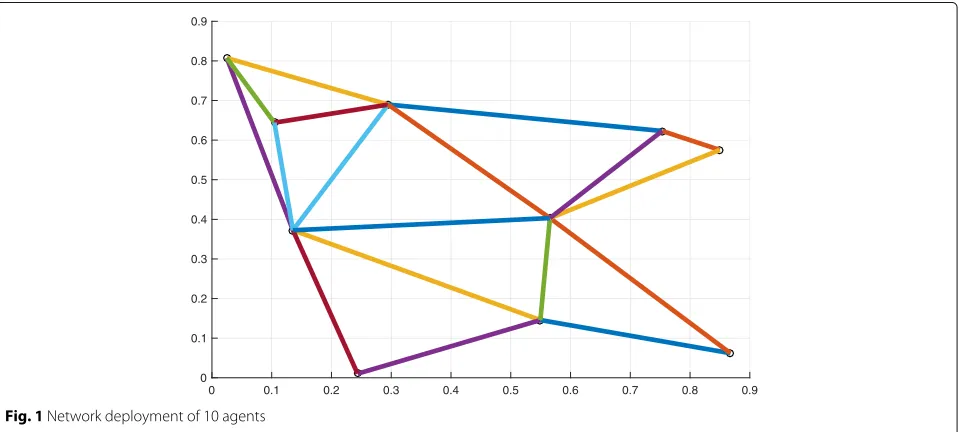
We generate a random geometric network of 10 agents, shown in Fig.1.

The relative degree6 of the graph is equal to 0.4. The graph was generated as a connected instance of the geo-metric graph model with radiusr = √ln(N)/N. To be specific, the first step involves generating 10 points in a unit square grid and the nodes are connected with a link if the distance between them is less than√ln(N)/N.

We repeat the procedure until we get a connected

graph instance. We choose the parameter set to be

= −π

4,π4

7 _{∈ R7}

. This choice of conforms

with Assumption 2. The sensing functions are

cho-sen to be certain trigonometric functions as described

below. The underlying parameter is set as θ =

[θ1, θ2, θ3, θ4, θ5, θ6, θ6] and thus θ ∈ R7. The sens-ing functions at the agents are taken to be, f1(θ) = sin(θ1 + θ2 + θ3),f2(θ) = sin(θ3 + θ2 + θ4),f3(θ) = sin(θ3 + θ4 + θ5),f4(θ) = sin(θ4 + θ5 + θ6),f5(θ) = sin(θ6 + θ5 + θ7),f6(θ) = sin(θ6 + θ7 + θ1),f7(θ) = sin(θ1 + θ2 + θ7),f8(θ) = sin(θ1 + θ2 + θ4),f9(θ) = sin(θ2+θ3+θ6)andf10(θ)= sin(θ3+θ4+θ6). Thus, it is to be noted that each node makes a scalar observation at timet. The noisesγn(t)are Gaussian and are i.i.d. both

in time and across nodes and have the covariance matrix equal to 0.25×I10. The local sensing functions render the parameterθ locally unobservable, but the parameter

θ is globally observable as, under the parameter set

considered in this setup, sin(·)is one-to-one and the set of

linear combinations of theθ components corresponding

to the arguments of the sin(·)’s constitute a full-rank system forθ. Hence, the global observability requirement

specified by Assumption 3 is satisfied. The unknown

but deterministic value of the parameter is taken to beθ = [π/6, −π/7,π/12, −π/5,π/16, 7π/36,π/10]. Under the model considered here in terms of the sensing

functions as specified above and the parameter set =

−π

4,π4 7

, it can be easily verified that the model conforms to the conditions specified in Assumptions3–7. The

pro-jection operator P onto the set defined in (14) is

given by,

0 0.1 0.2 0.3 0.4 0.5 0.6 0.7 0.8 0.9

0 0.1 0.2 0.3 0.4 0.5 0.6 0.7 0.8 0.9

[xn(t)]i=

⎧ ⎨ ⎩

π

4 [xn(t)]i≥ π4 [₋x_πn(t)]i −4π <[xn(t)]i< π4

4 [xn(t)]i< −4π,

(34)

for alli=1,· · ·,M.

The parameters of the two benchmarks and of the pro-posed estimator are as follows. The benchmark estimator in (13) has the consensus weight set to 0.48(t+1)−1_{. For} the proposed estimator, we setρt =0.45(t+1)−0.01and

ζt=(t+1)−0.49. The step size sequence for the benchmark

estimator proposed in [43] is set toμt=(0.3(t+20))−1.

It is to be noted that the Laplacian matrix considered for the benchmark estimator and the expected Laplacian

matrix for the proposed estimator, CREDO−N L are

equal, i.e.,L = L. The innovation weight is set toαt =

(0.3(t+20))−1. It is to be noted that with the time shifted innovation potential, the theoretical results in this paper continue to hold. As a performance metric, we use the relative MSE estimate averaged across nodes:

1 N

N

n=1

xn(t)−θ2

xn(0)−θ2

,

further averaged across 100 independent runs of the esti-mators. In the above equation,xn(0)refers to the initial

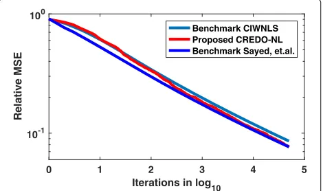
estimates at each node, which is set asxn(0)=0. Figure2

plots the relative MSE decay in terms of the number of iterations or the number of samples. It can be seen that the MSE decay of the two benchmark estimators and the

MSE decay of the proposed estimatorCREDO−N Lare

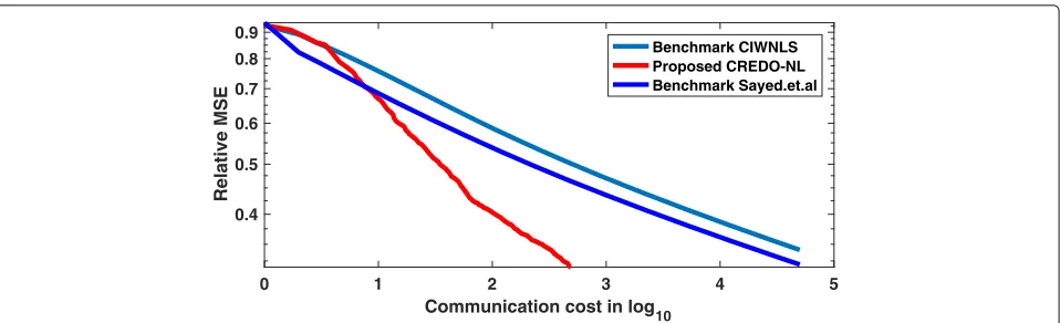
very similar with respect to the iteration count. Figure3 plots the MSE decay of the three estimators in terms of the communication cost per node. It can be seen for

0 1 2 3 4 5

Iterations in log₁₀ 10-1

100

Relative MSE

Benchmark CIWNLS Proposed CREDO-NL Benchmark Sayed, et.al.

Fig. 2Comparison of the proposed and benchmark estimators in

terms of relative MSE: Number of Iterations. The light blue line represents theCIWN LSalgorithm, the dark blue line represents the diffusion based algorithm proposed in [43], and the red line represents the proposed estimator

example that, at a relative MSE level of 10−1_{, the} pro-posed estimator requires 20 and 18 times less commu-nications as compared to the estimator in (13) and the algorithm in [43]. One can also notice a faster MSE decay

in terms of the communication cost forCREDO−N L

as compared to the benchmark (13), thus confirming our theory.

6 Discussion

In the context of existing work on non-linear dis-tributed methods, e.g., [15, 16, 31, 34–36, 40],

the current paper contributes by developing a

method with a strictly faster communication rate of O(1/C_t2−ζ)(ζ > 0 arbitrarily small) with respect to existing O(1/Ct) rates. Further, with respect to

existing works that develop methods designed to achieve communication efficiency, e.g., [13, 21, 44–46],

we develop here a different scheme with randomized

increasingly sparse communications. Finally, this paper is a continuation of works [37,38] but, in contrast with [37, 38], it considers non-linear observation models. This requires novel analysis techniques as detailed in Section1. It would be interesting to apply the proposed method on real data sets, e.g., in the context of IoT or power systems applications, in addition to synthetic data tests considered here.

7 Conclusions

In this paper, we have proposed CREDO−N L—a

communication-efficient distributed estimation scheme for non-linear observation models. We established strong consistency of the estimate sequence at each agent and characterized the MSE decay in terms of the per-agent

communication cost Ct. CREDO−N L achieves the

MSE decay rate OC_t−2+ζ, where ζ > 0 andζ is arbi-trarily small. Future research directions include extending the proposed algorithm to a mixed-time scale stochastic approximation type algorithm, so as to achieve an asymp-totic covariance independent of the network, as well as to extend the presented ideas to distributed stochastic optimization.

Endnotes

1_{From now on, in order to better distinguish the MSE}

rate of decay with respect to the number of iterationstand with respect to the number of per-node communications, we will refer to the former as theMSE iteration-wise rate and to the latter as theMSE communication rate.

0 1 2 3 4 5 Communication cost in log₁₀

0.4 0.5 0.6 0.7 0.8 0.9

Relative MSE

Benchmark CIWNLS Proposed CREDO-NL Benchmark Sayed.et.al

Fig. 3Comparison of the proposed and benchmark estimators in terms of relative MSE: Communication Cost Per Node. The light blue line

represents theCIWN LSalgorithm, the dark blue line represents the diffusion-based algorithm proposed in [43], and the red line represents the proposed estimator

of the benchmark estimator (13)-(14). As the proposed

CREDO−N Lestimator is single time scale,1 can be taken to be zero, and the main results (Theorems 1 and 2 ahead) continue to hold.

3_{To see this, note that the dependence of the}

measure-ments on the state is through sinusoidal functions (see Eq. (4)), which are everywhere differentiable and thus the gradient offn(·) within the domain exists

every-where. Moreover, as the derivatives of sin(·)and cos(·)are bounded, the norm of gradient offn(·)is bounded. Finally,

regarding Assumption3, it can be shown that the assump-tion is satisfied if (1) graph G is connected; (2) the set of admissible phase angle values, i.e., the parameter con-straint set, is chosen appropriately; (3) the real power flow between nodesnandlis non-zero if and only if there exists a physical transmission line connecting the nodes; and (4) voltage magnitudeVn =0, for all nodesn. Please

see Proposition 27 in [19].

4_{To see why this is true, consider for simplicity the}

caseRn = I, for alln. Then, there holds:nN=1fn(θ)− fn(θ)2 = (θ − θ) Nn=1FnFn

(θ − θ). Now, the statement of Assumption 3 becomes the following: the matricesFn,n = 1, ...,N, are such that there holds:(θ −

θ) N

n=1FnFn

(θ −θ) =0 if and only ifθ −θ. But this is equivalent to requiring thatN_n=1F_nFnis full rank.

5 _{Applied to our setting and in our notation, the}

diffu-sion method as in [43] takes the following form:

x_n(t+1)=xn(t)−μt(∇fn(xn(t)))R−n1(fn(xn(t))−yn(t))

xn(t+1)=

l∈n∪{n}

alnx_l(t+1).

Here,xn(t)is the solution estimate at agentn,xn(t)is an

auxiliary sequence at agentn,μtis the step-size, and the aln’s are combination weights that constitute together a

N×Ncolumn-stochastic matrix.

6_{Relative degree is the ratio of the number of links in}

the graph to the number of possible links in the graph.

Appendix A: Proof of Main Results

We present the proofs of main results in this section.

Proof of Theorem 4.1We start the proof with the follow-ing useful Lemma.

Lemma 1For each n, the process{xn(t)}satisfies

Pθ

& sup

t≥0

x(t)<∞ '

=1. (35)

ProofConsider (14). Since the projection is onto a com-pact convex set, it is non-expansive. It follows that the inequality

xn(t+1)−θ ≤ xn(t+1)−θ (36)

holds for allnandt. We first note that,

L(t)=βtL+L(t), (37)

whereEL(t)=0andE

L2_i,j(t)

= ρ02β0

(t+1)1+ − β 2 0

(t+1)2, for {i,j} ∈E,i=j.

Define, z(t) = x(t) − 1N ⊗θ and V(t) = z(t)2.

(Here, 1N is the all-ones N by 1 vector.) Note that z(t)

Lemma A1. Let{Ft}be the natural filtration generated by

the random observations and the random Laplacians i.e.,

Ft=σyn(s) N_n=1,{L(s)} braic manipulations, conditional independence, and uti-lizing (36), we have that,

wherezCdenotes the projection ofzto the consensus

sub-spaceC =z∈RMN|z=1N⊗a, for some a∈RM . The

Here, we recall thatλN(L) is the largest eigenvalue of

matrix L. Further, c1 is defined in Assumption 7, and

c2,c5 are appropriately chosen positive constants. Here,

zC⊥(t) = z(t)−zC(t), wherezC(t) is the projection of z(t) on the consensus subspaceC. Inequality (q0) holds

because, as noted above, there holds that E

(q3)follow from the properties of the Laplacian. Inequal-ity(q2)follows from Assumption7, and(q4)follows from Assumption 6 since we have that ∇fn(xn(t)) is uni-formly bounded from above by kn for alln, and hence,

we have thatG(x(t)) ≤ maxn=1,···,Nkn. (Recall quantity the noise process under consideration has finite covari-ance. We also use the fact that, almost surely,G(x(t)) ≤

lows from the Lipschitz continuity in Assumption6and

the result that G(x(t)) ≤ maxn=1,···,Nkn. That is, c3 may be taken as(maxn=1,···,Nkn)4(maxn=1,···,NR−n1)2.

Applying the bounds (41)–(43) in (39), we obtain, after some algebraic manipulations,

where c6,c8,c9 are appropriately chosen positive con-stants, andc5is as in (41). In particular,c6may be taken as

Hence,{W(t)} is a non-negative supermartingale and

converges a.s. to a bounded random variableW∗ast →

∞. It then follows from (46) thatV(t) →W∗ast → ∞. Thus, we conclude that the desired claim holds.

The following Lemma will play a key role in establishing the convergence of the estimate sequence.

Lemma 2(Lemma 4.1 in [18])Consider the scalar time-varying linear system

where{r1(t)}is a sequence, such that

We now prove the almost sure convergence of the esti-mate sequence to the true parameter. Following similar steps as in the proof of Lemma1, fortlarge enough

E[V(t+1)|Ft]≤1−2c1αt+c7αt2 is bounded from above. Moreover, it also follows that {V1(t)}t≥t1 is a supermartingale and hence converges a.s. to a finite random variable. By definition from (53), we also have that {V(t)} converges to a non-negative finite random variableV∗. Finally, from (52), we have that, non-negativity of the sequence{V(t)}, we conclude that

0≤E[V∗]≤lim inf

t→∞ E[V(t)]=0, (55)

which thus implies thatV∗ = 0 a.s. Hence,z(t) → 0 a.s. ast→ ∞, and the desired assertion follows.

We will use the following approximation result (Lemma3) and the generalized convergence criterion (Lemma4) for

the proof of Theorem 2. Lemma 3 is an extension of

Lemma 5 in [18]. Lemma4is Lemma 10 in [8].

Lemma 3Let{bt}be a scalar sequence satisfying

bt+1≤

Proof of Theorem 4.2Consider inequality (54), and recall that, by Assumption8, we have thatα0c1> 1. We can now see that the sequence{V(t)}then falls under the purview of Lemma3, and we have

lim sup

Inequality (58) now clearly implies that, for each agent n, there holds:

The communication cost Ct for the proposed

CREDO−N Lalgorithm is given byCt =

t+12

, and thus the assertion follows in conjunction with (59).

Abbreviations

CPS: Cyber-physical systems;CREDO: Communication efficient REcursive Distributed estimatOr;CREDO−N L:CREDO-non-linear; i.i.d.: Independent identically distributed; IoT: Internet of things

Funding

This work is supported by the I-BiDaaS project, funded by the European Commission under Grant Agreement No. 780787. This publication reflects the views only of the authors, and the Commission cannot be held responsible for any use which may be made of the information contained therein. The work of D. Jakovetic is also supported in part by the Serbian Ministry of Education, Science, and Technological Development, grant 174030. The work is also partially supported by the National Science Foundation under grant CCF-1513936.

Availability of data and materials

The data used in this paper is synthetic and is generated as described in Section 5 of the paper. Please contact authors for data requests.

Authors’ contributions

AKS lead the writing of Sections 2–5 and Appendix, he also lead carrying out theoretical analysis, and he carried out numerical experiments in Section 5. He also contributed in writing Sections 1, 6, and 7. DJ lead the writing of Sections 1, 6, and 7. He also contributed in writing Sections 2–5 and Appendix and in developing the code for carrying out numerical results in Section 5. DB contributed in writing Sections 1–4. SK contributed in writing Sections 1–3 and Appendix. All authors read and approved the final manuscript.

Ethics approval and consent to participate

Consent for publication

Not applicable.

Competing interests

The authors declare that they have no competing interests.

Publisher’s Note

Springer Nature remains neutral with regard to jurisdictional claims in published maps and institutional affiliations.

Author details

1_{Department of Electrical and Computer Engineering, Carnegie Mellon}

University, Pittsburgh, USA.2University of Novi Sad, Faculty of Sciences, Department of Mathematics and Informatics, 21000 Novi Sad, Serbia. 3_{University of Novi Sad, Faculty of Technical Sciences, Department of Power,}

Electronic and Communication Engineering, 21000 Novi Sad, Serbia.

Received: 23 March 2018 Accepted: 24 September 2018

References

1. A. Abur, A. G. Exposito,Power System State Estimation: Theory and Implementation. (Marcel Dekker, New York, 2004)

2. D. Bajovi´c, J. M. F. Moura, J. Xavier, B. Sinopoli, Distributed inference over directed networks: performance limits and optimal design. IEEE Trans. Sig. Process.64(13), 3308–3323 (2016)

3. B. Bollobas,Modern Graph Theory. (Springer Verlag, New York, 1998) 4. P. Braca, S. Marano, V. Matta, Enforcing consensus while monitoring the

environment in wireless sensor networks. IEEE Trans. Sig. Process.56(7), 3375–3380 (2008)

5. F. Cattivelli, A. H. Sayed, Diffusion LMS strategies for distributed estimation. IEEE Trans. Sig. Process.58(3), 1035–1048 (2010) 6. J. Chen, C. Richard, A. H. Sayed, Multitask diffusion adaptation over

networks. IEEE Trans. Sig. Process.62(16), 4129–4144 (2014)

7. F. R. K. Chung,Spectral graph theory, vol. 92. (American Mathematical Soc., Providence, 1997)

8. L. E. Dubins, D. A. Freedman, A sharper form of the Borel-Cantelli lemma and the strong law. Ann. Math. Stat.36(3), 800–807 (1965)

9. V. Fabian, On asymptotically efficient recursive estimation. Ann. Stat.6(4), 854–866 (1978)

10. R. Z. Has’minskij, inProc. Prague Symp. Asymptotic Statist.Sequential estimation and recursive asymptotically optimal procedures of estimation and observation control, vol. 1 (Charles Univ., Prague, 1974), pp. 157–178 11. C. Heinze, B. McWilliams, N. Meinshausen, in19th International Conference

on Artificial Intelligence and Statistics. Dual-loco: distributing statistical estimation using random projections, (Cadiz, 2016), pp. 875–883 12. M. D. Ilic’, J. Zaborszky,Dynamics and Control of Large Electric Power

Systems. (Wiley, New York, 2000)

13. D. Jakovetic, D. Bajovic, N. Krejic, N. Krklec Jerinkic, Distributed gradient methods with variable number of working nodes. IEEE Trans. Sig. Process.

64(15), 4080–4095 (2016)

14. D. Jakovetic, J. Xavier, J. M. F. Moura, Cooperative convex optimization in networked systems: augmented Lagrangian algorithms with directed gossip communication. IEEE Trans. Sig. Process.59(8), 3889–3902 (2011) 15. R. I. Jennrich, Asymptotic properties of non-linear least squares

estimators. Ann. Math. Stat.40(2), 633–643 (1969)

16. S. Kar, J. M. F. Moura, Asymptotically efficient distributed estimation with exponential family statistics. IEEE Trans. Inf. Theory.60(8), 4811–4831 (2014)

17. S. Kar, J. M. F. Moura, H. V. Poor, Distributed linear parameter estimation: asymptotically efficient adaptive strategies. SIAM J. Control Optim.51(3), 2200–2229 (2013)

18. S. Kar, J. M. F. Moura, H. V. Poor, QD-Learning: A Collaborative Distributed Strategy for Multi-Agent Reinforcement Learning Through Consensus + Innovations. IEEE Trans. Signal Process.61(7), 1848–1862 (2013) 19. S. Kar, J. M. F. Moura, K. Ramanan, Distributed parameter estimation in

sensor networks: nonlinear observation models and imperfect communication. IEEE Trans. Inf. Theory.58(6), 3575–3605 (2012) 20. S. Kar, J. M. F. Moura, Convergence rate analysis of distributed gossip

(linear parameter) estimation: fundamental limits and tradeoffs. IEEE J. Sel. Top. Sig. Process.5(4), 674–690 (2011)

21. G. Lan, S. Lee, Y. Zhou, Communication-efficient algorithms for decentralized and stochastic optimization. arXiv preprint arXiv:1701.03961 (2017)

22. J. Li, A. H. Sayed, Modeling bee swarming behavior through diffusion adaptation with asymmetric information sharing. EURASIP J. Adv. Sig. Process.18(1), 2012

23. Q. Liu, A. T. Ihler, inNIPS’14 Proceedings of the 27th International Conference on Neural Information Processing Systems - Volume 1. Distributed estimation, information loss and exponential families (MIT Press, Cambridge, 2014), pp. 1098–1106

24. C. G. Lopes, A. H. Sayed, Diffusion least-mean squares over adaptive networks: formulation and performance analysis. IEEE Trans. Sig. Process.

56(7), 3122–3136 (2008)

25. P. D. Lorenzo, A. H. Sayed, Sparse distributed learning based on diffusion adaptation. IEEE Trans. Sig. Process.61(6), 1419–1433 (2013)

26. C. Ma, M. Takáˇc, Partitioning data on features or samples in communication-efficient distributed optimization? arXiv preprint arXiv:1510.06688 (2015)

27. C. Ma, V. Smith, M. Jaggi, M. Jordan, P. Richtarik, M. Takac, inICML’15 Proceedings of the 32nd International Conference on International Conference on Machine Learning - Volume 37. Adding vs. averaging in distributed primal-dual optimization, (Lille, 2015), pp. 1973–1982 28. G. Mateos, G. B. Giannakis, Distributed recursive least-squares: stability and

performance analysis. IEEE Trans. Sig. Process.60(7), 3740–3754 (2012) 29. G. Mateos, I. Schizas, G. B. Giannakis, Performance analysis of the

consensus-based distributed LMS algorithm. EURASIP J. Adv. Sig. Process.

68, 2009 (2009)

30. A. Nedi´c, A. Olshevsky, C. Uribe, in2015 American Control Conference (ACC). Nonasymptotic convergence rates for cooperative learning over time-varying directed graphs (IEEE, Chicago, 2015).https://doi.org/10. 1109/ACC.2015.7172262

31. A. Nedic, A. Ozdaglar, Distributed subgradient methods for multi-agent optimization. IEEE Trans. Autom. Control.54(1), 48–61 (2009) 32. J. Pfanzagl, inProceedings of the Prague Symposium on Asymptotic

Statistics, ed. by J. Hajek. Asymptotic optimum estimation and test procedures, vol. 1 (Charles University, Prague, 1974), pp. 201–272 33. A. Primadianto, C. N. Lu, A review on distribution system state estimation.

IEEE Trans. Power Syst.32(5), 3875–3883 (2017)

34. S. S. Ram, A. Nedic, V. V. Veeravalli, Incremental stochastic subgradient algorithms for convex optimization. SIAM J. Optim.20(2), 691–717 (2009) 35. S. S. Ram, A. Nedi´c, V. V. Veeravalli, Distributed stochastic subgradient

projection algorithms for convex optimization. J. Optim. Theory Appl.

147(3), 516–545 (2010)

36. S. S. Ram, V. V. Veeravalli, A. Nedic, Distributed and recursive parameter estimation in parametrized linear state-space models. IEEE Trans. Autom. Control.55(2), 488–492 (2010)

37. A. K. Sahu, D. Jakovetic, S. Kar, Communication optimality trade-offs for distributed estimation. arXiv preprint arXiv:1801.04050 (2018) 38. A. K. Sahu, D. Jakovetic, S. Kar, inInternational Symposium on Information

Theory, ISIT. CREDO: A communication-efficient distributed estimation algorithm, (Vail, 2018)

39. A. K. Sahu, S. Kar, Distributed sequential detection for Gaussian shift-in-mean hypothesis testing. IEEE Trans. Sig. Process.64(1), 89–103 (2016)

40. A. K. Sahu, S. Kar, J. M. F. Moura, H. V. Poor, Distributed constrained recursive nonlinear least-squares estimation: algorithms and asymptotics. IEEE Trans. Sig. Inf. Process. Over Networks.2(4), 426–441 (2016) 41. D. J. Sakrison, Efficient recursive estimation; application to estimating the

parameters of a covariance function. Int. J. Eng. Sci.3(4), 461–483 (1965) 42. C. J. Stone, Adaptive maximum likelihood estimators of a location

parameter. Ann. Stat.3(2), 267–284 (1975)

43. Z. J. Towfic, J. Chen, A. H. Sayed, Excess-risk of distributed stochastic learners. IEEE Trans. Inf. Theory.62(10), 5753–5785 (2016) 44. K. Tsianos, S. Lawlor, M. G. Rabbat, inNIPS’12 Proceedings of the 25th

International Conference on Neural Information Processing Systems -Volume 2. Communication/computation tradeoffs in consensus-based distributed optimization (Curran Associates Inc., Lake Tahoe, 2012), pp. 1943–1951

46. Z. Wang, Z. Yu, Q. Ling, D. Berberidis, G. B. Giannakis, Decentralized RLS with data-adaptive censoring for regressions over large-scale networks. IEEE Trans. Signal Proc.66(6) (2018)

47. Y. Zhang, J. Duchi, M. Wainwright, inProceedings of the 26th Annual Conference on Learning Theory, PMLR. Vol. 30. Divide and conquer kernel ridge regression, (Princeton, 2013), pp. 592–617