Soft and Joint Source Channel Decoding of Quasi Arithmetic Codes

Soft and Joint Source-Channel Decoding

of Quasi-Arithmetic Codes

Thomas Guionnet

Projet TEMICS, IRISA-INRIA, Campus Universitaire de Beaulieu, 35042 Rennes Cedex, France Email:[email protected]

Christine Guillemot

Projet TEMICS, IRISA-INRIA, Campus Universitaire de Beaulieu, 35042 Rennes Cedex, France Email:[email protected]

Received 20 November 2002; Revised 7 August 2003; Recommended for Publication by Antonio Ortega

The issue of robust and joint source-channel decoding of quasi-arithmetic codes is addressed. Quasi-arithmetic coding is a reduced precision and complexity implementation of arithmetic coding. This amounts to approximating the distribution of the source. The approximation of the source distribution leads to the introduction of redundancy that can be exploited for robust decoding in presence of transmission errors. Hence, this approximation controls both the trade-offbetween compression efficiency and com-plexity and at the same time the redundancy (excess rate) introduced by this suboptimality. This paper provides first a state model of a quasi-arithmetic coder and decoder for binary andM-ary sources. The design of an error-resilient soft decoding algorithm follows quite naturally. The compression efficiency of quasi-arithmetic codes allows to add extra redundancy in the form of mark-ers designed specifically to prevent desynchronization. The algorithm is directly amenable for iterative source-channel decoding in the spirit of serial turbo codes. The coding and decoding algorithms have been tested for a wide range of channel signal-to-noise ratios (SNRs). Experimental results reveal improved symbol error rate (SER) and SNR performances against Huffman and optimal arithmetic codes.

Keywords and phrases:robust arithmetic and quasi-arithmetic coding, joint source-channel coding, soft decoding, estimation, MAP.

1. INTRODUCTION

Entropy coding, producing variable length codewords (VLCs), is a core component of any data compression scheme. However, VLCs are very sensitive to channel noise: when some bits are altered by the channel, synchroniza-tion losses can occur at the receiver, the posisynchroniza-tion of symbol boundaries are not properly estimated, leading to dramatic symbol error rates (SERs). This phenomenon has given mo-mentum to extensive work on the design of procedures for soft decoding and joint source-channel decoding of VLCs. Soft VLC decoding ideas, exploiting residual source redun-dancy (the so-called excess rate), have also been shown to reduce the “desynchronization” effect as well as the resid-ual bit error rate and SER [1,2,3]. Models incorporating both VLC-encoded sources and channel codes (CCs) have also been considered [4,5,6,7].

The research effort has first focused on Huffman codes [3, 4, 5, 8] and on reversible VLCs [6, 9, 10]. However, arithmetic codes have gained increased popularity in

code [16]. Sequential decoding of arithmetic codes is inves-tigated in [17] for supporting error correction capabilities. The complexity of this approach is reduced in [18] by us-ing trellis-coded modulation combined with a list Viterbi de-coding algorithm. A soft dede-coding procedure is described in [19]. However, one difficulty comes from the fact that the code tree, hence the state-space dimension, or the number of states of the model grows exponentially with the number of symbols being encoded. A pruning technique is then used to limit the complexity within a tractable and realistic range. However, it brings inherent limitations when using the de-coder in an iterative source-channel decoding structure. The pruning of the tree to limit the complexity is such that, in this particular case, the iterations do not bring a significant gain.

A fast arithmetic coding procedure called quasi-arith-metic codinghas been introduced in [20]. It operates on an integer interval [0,T[ and on integer subdivisions of this in-terval. This amounts to approximate the source distribution. This controlled approximation allows to reduce the number of possible coder states without significantly degrading the compression performance. The trade-offbetween the state-space dimension and the source distribution approximation is controlled by the parameter T. IfT is sufficiently small, all state transitions and outputs can then be precomputed and table lookups be in turn substituted for arithmetic oper-ations. A quasi-arithmetic coder can be regarded as an arith-metic coder governed by an approximation of the real source distribution.

In this paper, we first revisit finite-state automaton mod-eling of quasi-arithmetic coding and decoding processes for

M-ary sources. Notice that theM-ary source could be coded directly with a quasi-arithmetic coder. An accurate approxi-mation of theM-ary source distribution would however re-quire to set the parameter T to a high value, resulting in a high state-space dimension, hence in high decoding com-plexity. To maintain the complexity within a tractable range, one would have to rely on a very coarse source distribu-tion approximadistribu-tion. One can instead first map the M-ary source model into a binary model by means of a fixed-length binary code represented as a binary tree with symbols at the leaves. These trees are connected up to a depth function of the source model (e.g., for an order-1 Markov source, the depth is one). Leaves of the tree represent terminated sym-bols and are identified with the root of the next tree. The resulting finite binary tree can be regarded as a stochastic au-tomaton that models the source symbol distribution. Once theM-ary source has been converted into a binary source, the latter can be encoded by a quasi-arithmetic coder. The transitions on the binary model govern the quasi-arithmetic coder. The design of an efficient estimation procedure based on the BCJR algorithm [21] follows quite naturally. The de-coding complexity remains within a realistic range without the need for applying any pruning of the estimation trellis. The estimation algorithm has been validated under various channel conditions and for different levels of source corlation. Experimental results have shown very high error re-silience while at the same time preserving a very good

com-pression efficiency. For a comparable overall rate, in compar-ison with Huffman codes, better compression efficiency of quasi-arithmetic codes allows to dedicate extra redundancy (short “soft” synchronization patterns) specifically to de-coder resynchronization, resulting in significantly higher er-ror resilience. The usage of CCs is also considered in order to reduce the bit error rate seen by the source estimation algo-rithm. The latter can then be placed in an iterative decoding structure in the spirit of serially concatenated turbo codes, provided that the channel decoder and the quasi-arithmetic decoder are separated by an interleaver. Since, in contrast with optimal arithmetic coding, the estimation can be per-formed without pruning the trellis, the potential of the iter-ative decoding structure can be fully exploited, resulting in a very low SER (significantly lower than what can be obtained with Huffman codes). Overall, the great flexibility that quasi-arithmetic codes offer for adjusting compression efficiency, error resilience, and complexity allows an optimal adapta-tion to various transmission condiadapta-tions and terminal capa-bility requirements.

The rest of the paper is organized as follows.Section 2 describes the notations we use and states the problem ad-dressed. Sections3and4review the principles of arithmetic and quasi-arithmetic coding. Sections5and6address mod-eling issues of, respectively, coding/decoding processes and of the source. This material is exploited in the sequel (Sections 7and8) for explaining the estimation algorithm and the soft synchronization procedure.Section 9outlines the construc-tion of the iterative joint source-channel decoding procedure based on quasi-arithmetic codes. Finally, experimental re-sults are described inSection 10. We first compare the perfor-mance of the algorithm in terms of SER and signal-to-noise ratio (SNR) with respect to soft Huffman and arithmetic de-coding with theoretical Gauss-Markov sources. Simulations results of the joint source-channel turbo decoding algorithm in comparison with soft decoding of quasi-arithmetic codes are also provided.

2. NOTATIONS AND PROBLEM STATEMENT

LetA= A1· · ·ALbe a sequence of quantized source sym-bols taking their values in a finite alphabet Ꮽcomposed of

M =2qsymbols,Ꮽ= {a1,a2,. . .,ai,. . .,aM}. The sequence

M-ary source

Figure1: Conversions taking place in the coding chain.

3. ARITHMETIC CODING PRINCIPLES

We first review the principle of arithmetic coding on a simple example of a source taking values in the alpha-bet {a1,a2,a3,a4} with the stationary distribution Pa = [0.6, 0.2, 0.1, 0.1]. The interval [0, 1[ is partitioned into four cells representing the four symbols of the alphabet. The size of each cell is the stationary probability of the correspond-ing symbol. The partition (hence the bounds of the diff er-ent segmer-ents) of the unit interval is given by the cumula-tive stationary probability of the alphabet symbols. The in-terval corresponding to the first symbol to be encoded is chosen. It becomes the current interval and is again parti-tioned into different segments. The bounds of the resulting segments are driven by the model of the source. Consider-ing an order-1 Markov chain, these bounds will be governed byP(A_l+1|Al), hence, in this particular case, will be function of both the probability of the previous symbol and of the cumulative probability of the alphabet symbols. Therefore, the arithmetic coder adapts in this case to the entropyrate H(A_l+1|Al) of processA, that is, it compresses the innova-tion of the Markov chainA.

In the example above, when the sequencea1,a4,a2,a1 has been encoded, the current interval is [0.576, 0.5832[. Any number in this interval can be used to identify the sequence. We consider 0.576. The decoding of the sequence is per-formed by reproducing the coder behavior. First, the interval [0, 1[ is partitioned according to the cumulative probability of the source. Since the value 0.576 belongs to the interval [0, 0.6[, it is clear that the first symbol encoded has beena1. Therefore, the first symbol is decoded and the interval [0, 0.6[ is partitioned according to the cumulative probability of the source. The process is repeated until full decoding of the se-quence. Practical implementations of arithmetic coding have been first introduced in [22,23] and developed further in [24]. One problem that may arise when implementing arith-metic coding is the high precision needed to represent very small real numbers. In order to overcome this difficulty, one can base the algorithm on the binary representation of real numbers in the interval [0, 1[ (see [25]). Any number in the interval [0, 0.5[ will have its first bit equal to 0, while any number in the interval [0.5, 1[ will have its first bit equal to 1. Therefore, during the encoding process, as soon as the cur-rent interval is entirely under or over 1/2, the corresponding bit is emitted and the interval length is doubled. There is a specific treatment for the intervals straddling 1/2. When the current interval straddles 1/2 and is in [0.25, 0.75[, it can-not be identified by a unique bit. Its size is therefore doubled without emitting any bit, and the number of rescaling op-erations taking place before emitting any bit is memorized. When reaching an interval for which one bitU_i=uican be

emitted, then this bit will be followed by a number of bits

Ui+1 =ui+1· · ·Ui+n =ui+1, wherenis the number of scal-ing operations that have been performed before the emis-sion ofUi, and whereui+1 = ui+ 1 mod 2. The use of this technique guarantees that the current interval always satisfies low <0.25<0.5≤high or low <0.5<0.75≤high, where low and high are, respectively, the lower and upper bounds of the current interval. This avoids the problems of preci-sion which may otherwise occur in the case of small intervals straddling the middle of the segment [0, 1[.

4. FAST-REDUCED PRECISION IMPLEMENTATION

Arithmetic coding is near optimality in terms of compres-sion. Error-resilient decoding solutions can be designed [19], however, their complexity can be an issue in some contexts. The coding process can indeed be modeled under the form of a stochastic automaton, where the states are defined by three variables: low, up (denoting the bounds of the subinterval resulting from successive subdivisions of the interval [0, 1[), andnscl denoting the number of scalings performed since the last emitted bit, as explained inSection 3. Subdivisions of the interval [low, up[, hence next states, are functions of the cumulative probability distribution of the source. With-out the source model, the possible number of subdivisions, hence of states, may be infinite. If the source distribution is known, the number of states still grows exponentially with the number of symbols being encoded.

4.1. Quasi-arithmetic coding

It is observed in [20] that controlled approximations can reduce the number of possible states without significantly degrading compression performance. All state transitions and outputs can then be precomputed and table lookups can be used instead of arithmetic operations. This fast, but reduced precision, implementation of arithmetic coding is calledquasi-arithmetic coding[20]. Instead of using the real interval [0, 1[, quasi-arithmetic coding is performed on an integer interval [0,T[. The value ofTcontrols the trade-off between complexity and compression efficiency: ifTis suffi -ciently large, then the interval subdivisions will follow closely the distribution of the source. In contrast, ifTis small, all the interval subdivisions can be precomputed.

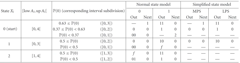
Table1: Quasi-arithmetic coder states, transitions, and outputs forT=4.

Normal state model Simplified state model StateXl [lowAl, upAl[ P(0) (corresponding interval subdivision) 0 1 MPS LPS

Out Next Out Next Out Next Out Next

0 (start) [0, 4[

0.63≤P(0) ([0, 3[) — 1 11 0 — 1 11 0

0.37≤P(0)<0.63 ([0, 2[) 0 0 1 0 0 0 1 0

P(0)<0.37 ([0, 1[) 00 0 — 2 — — — —

1 [0, 3[ 0.5≤P(0) ([0, 2[) 0 0 10 0 0 0 10 0

P(0)<0.5 ([0, 1[) 00 0 f 0 — — — —

2 [1, 4[ 0.5≤P(0) ([1, 3[) f 0 11 0 — — — —

P(0)<0.5 ([1, 2[) 01 0 1 0 — — — —

on the tree (or transitions between states) follow the dis-tribution of the source (P(A_l|Al−1) for an order-1 Markov source orP(A_l) in the zeroth-order case). LetX_ldenote the state of the automaton at each symbol instant l. As in the case of optimal arithmetic coding, the stateXlof the quasi-arithmetic coder is defined by three variables: lowA_l, upA_l, andnscl_l. The terms lowA_land upA_ldenote the bounds of the subinterval resulting from successive subdivisions of the interval [0,T[ triggered by the encoding of the sequenceAl₁. The quantitynscllis (re)set to zero when a bit is emitted and incremented each time a rescaling takes place. Hence, this quantity denotes the number of scalings performed since the last emitted bit. When a bit is emitted, it is followed bynscl_l bits of opposite value (seeSection 3).

Since there is a finite number of possible integer sub-divisions of the interval [0,T[, all the possible states of the quasi-arithmetic coder can be precomputed without knowl-edge of the source. This is however without accounting for the variablenscll. Indeed, the variablenscllis not bounded. The solution is then to consider nscl_l as a variable result-ing from state transitions (output variable) and not to con-sider this variable in the precomputation of the coder states. Table 1gives the states, outputs, and all possible transitions of a quasi-arithmetic coder precomputed for a binary source with T = 4. The value of the variable nscl_l is not consid-ered in this state model. Only the action of incrementing this variable when a rescaling is taking place is signalled by the letter f in the table, also referred to asfollow upin [26]. The coder has three states corresponding to integer subdivisions of the interval [0, 4[. The subdivisions that can possibly take place next are functions of the source probability distribu-tion. They are chosen in such a way that the correspond-ing distribution approximation will minimize the excess rate [26]. For example, we assume that the automaton is in state

Xl = 1 (defined by the interval [lowAl, upAl[ = [0, 3[). Depending on the probability of the input binary symbol 0, the interval [0, 3[ will be further subdivided into [0, 2[ corresponding to an approximated probability of 2/3 if its probability is higher than 1/2, or into [0, 1[ corresponding to an approximated probability of 1/3 if its probability is lower than 1/2. Both subdivisions result, after appropriate bit emission and scaling, into the state 0. The number of

possi-ble statesX_lis 3T2_{/16. If we take into account the different} source distributions, the number of possibletransitionsfrom all the statesX_lis 9T3_/64−6T2_{/32 +T/4.}

The number of states can be further reduced by identify-ing the symbols as more probable (MPS) and less probable (LPS) rather than as 1 and 0. This amounts to reducing the number of possible combinations of the binary source prob-abilities, the MPS being either the symbol 0 or the symbol 1. This allows to combine transitions and eliminate states as shown inTable 1. The sequenceX0· · ·XLis a Markov chain and the output of the coder is the function of transitions of this chain. This state representation can help designing a ro-bust maximum a posteriori (MAP) decoder. For a deeper un-derstanding of quasi-arithmetic coding, the reader may refer to [20].

4.2. Quasi-arithmetic decoding

We first consider the operation of an optimum arithmetic decoder. A sequence of arithmetically coded bitsU₁N is trans-lated into a sequence of symbols AL₁ by a binary decision tree. Each bit determines the choice of a vertex in the tree. Each node νof the tree identifies a state of the arithmetic decoder and corresponds to a tuple U1n−1 from which two transitions are possible: U_n = 0 or U_n = 1. The state of the decoder is specified by two intervals: [lowU_n, upU_n[ and [lowALn, upALn[. The interval [lowUn, upUn[ defines the

segment of the interval [0, 1[ selected by a given input bit se-quenceU1n. The interval [lowALn, upALn[ relates to the

sub-division obtained when the symbolA_Lncan be decoded with-out ambiguity. Both intervals must be scaled appropriately in order to avoid numerical precision problems. However, in contrast to the coding process, there is no need to keep track of the scalings that have been performed.

We now consider the interval [0,T[ and finite interval subdivisions. The quasi-arithmetic decoder can also be ex-pressed in the form of an automaton. Let X_n be its state at bit instantn;Xnstores the four variables [lowUn, upUn[ and [lowALn, upALn[. Since there is a finite number of

Table2: Quasi-arithmetic decoder states, transitions, and outputs forT=4.

StateXn State variables P(MPS) (corresponding subdivision of [lowALn, upALn[) Un=

0 Un=1

Out Next Out Next

0 (start) [lowUn, upUn[=[0, 4[ 0.63≤P(MPS) ([0, 3[) MPS, MPS 0 — 1

[lowALn, upALn[=[0, 4[ 0.37≤P(MPS)<0.63 ([0, 2[) MPS 0 LPS 0

1 [lowUn, upUn[=[2, 4[ 0.63≤P(MPS) ([0, 3[) MPS, LPS 0 LPS 0

[lowALn, upALn[=[0, 4[

andT = 4, with the MPS/LPS simplification. The decoder in this particular example has two states. Further subdivi-sions that will lead to transitions to next states are func-tions of the source probability distribution (e.g.,P(MPS) in Table 2). We assume, for example, that the automaton is in stateX_n=0 (defined by the two intervals [lowU_n, upU_n[=

[0, 4[ and [lowA_Ln, upA_Ln[ = [0, 4[), and that the input is

Un = 0. Depending on the probability of the source to be coded (hence here of the MPS and LPS symbols), the inter-val [0, 4[ will be further subdivided into [0, 3[ (if MPS prob-ability is higher than 0.63) or into [0, 2[ (if MPS probabil-ity is lower than 0.63), both subdivisions resulting into the state 0.

4.3. Source distribution approximation

Arithmetic coding realizes a conversion of source distribu-tions: in the general case, it realizes a conversion of a se-quence of symbols of anM-ary source of a given distribution into a sequence of symbols of a binary source with an inde-pendent and uniform distribution. A quasi-arithmetic coder does not produce a sequence of independently and uniformly distributed bits due to the approximation of the source dis-tribution that it realizes. It has been shown in [26] that this approximation does not induce a significant increase in code length. This however depends on the source statistics. This statement is true if the symbol probabilities are comprised between 1/tand (t−1)/t, wheretis the width of the current interval to be subdivided. Hence, the choice of the value of

Tmay depend on the source distribution. The excess rate re-sulting from the approximation can be computed as follows. Letabe a symbol taking its value inᏭ,P(a) the probability of the eventa, andQ(a) the approximation ofP(a) made by the quasi-arithmetic coder. The entropy of the source is given by

H= −

aM

a=a1

P(a) log₂P(a). (1)

The performance of the quasi-arithmetic coder can then be measured by

R= −

aM

a=a1

P(a) log₂Q(a). (2)

The excess rate induced by the quasi-arithmetic coder can hence be expressed as

E=R−H

=

aM

a=a1

P(a) log₂ P(a) Q(a)

=DPQ,

(3)

whereD(PQ) is the Kullback-Leibler distance or relative en-tropy between the approximate distributionQand the true distributionP.

5. SOURCE MODEL

For a binary source, the variableTcan be limited to a small value (down to 4) at a small cost in terms of compression [26]. This motivates a conversion of theM-ary source into a binary source to be then encoded by the quasi-arithmetic coder. This conversion amounts to a fixed-length binary cod-ing of the source.

We first assume that the source quantized onM = 2q symbols is an order-0 Markov source. It can then be repre-sented by a binary tree of depthq, as shown inFigure 2afor

M=4. The transition probabilities on the binary tree can be computed easily from the distribution of the source. The re-sulting binary tree can be seen as an automaton that models theM-ary source stationary distribution. A complete model of the source can be obtained by connecting thesuccessive lo-cal models. One possible solution consists in identifying the leafnodes of the binary tree with the rootnode of the next tree. This leads to the three states automaton ofFigure 2bin the particular case of an order-0 Markov source withM=4. InFigure 2c, the same automaton is shown in the form of a trellis, with the probability of each bit indicated on the cor-responding transition. Relying on this stochastic automaton model, the sequence of the resulting binary symbols can be modeled as a function of a hidden Markov model. LetCk de-note the stateνof the automaton afterkbinary symbols have been produced. The sequenceC0,. . .,CK is a Markov chain, and the resulting sequence of binary symbols is a function of transitions of this chain, that is,S_k=φ(C_k−1,Ck).

We now assume that the source is an order-1 Markov source. To take into account the correlation present in the

M-ary source, in the model construction, one must in addi-tion keep track of the lastM-ary symbol coded. In order to do so, one could define the state variableC_kas a pair (ν,σ), where σ is the value of the last completed symbol Al and

0 0

1

1 0

1

a1(0.1)

a2(0.4)

a3(0.4)

a4(0.4)

(a)

0

0 1

0 1

1 (b)

0(0.5) 1(0.5)

0(0.2) 1(0.8)

0(0_.8) 1(0.2)

(c)

Figure2: Graphical representation under the form of (a) a tree, (b) a stochastic automaton, and (c) a trellis of the binary model of the order-0 Markov source. Black dots correspond to leafnodes identified to rootnodes of next trees. White dots correspond to intermediate nodes of the binary representation of theM-ary symbols (M=4).

0

0 a

1

0 0

a2

1

1 0

1

1 ₀

1

a1

a2

a3

a4

a3

a4

(a)

0

0

a1

0 1

1 0

a2

1 0 1

0 a

3

1 1

a4

(b)

Figure3: Graphical representation under the form of (a) a tree and (b) a stochastic automaton of the binary model of the order-1 Markov source (M=4).

P(A_l+1|Al). Alternately, one can take into account the con-ditional distributionP(A_l+1|Al), by connectingM+ 1 trees of depthqas shown inFigure 3a, and define the state vari-ableCkas a nodeνin the resulting tree. The complete model of the source is then obtained by additional transitions from leaves to intermediate nodes as shown inFigure 3b. In this particular case, the model leads to a state space of dimension 15. The state-space dimension for an order-nMarkov source quantized onMsymbols is given byMn+1_{−1. For both state} models (C_k =(ν,σ) andC_k =(ν)), the sequenceC1· · ·CK is a Markov process, the transitions of which produce the se-quenceSof binary symbols.

Remark1. The construction of the binary model, that is, the assignment of the binary codewords to the different

sym-bols, has a strong impact on the reliability of the estimation. The transition probabilities on the binary tree are indeed defined by this symbol-to-leave assignment. Increased esti-mation reliability can be obtained when the different paths (or branches) on the model have a highly nonuniform like-lihood, that is, when the uncertainty of some branches is much lower than for others. The assignment of binary code-words to symbols must hence be such that the expression

search space to a subset of index assignments. In the experi-ments reported here, this subset has been obtained by a sim-ple circular shift of an initial index assignment. This initial-ization has an impact on the resulting SER and SNR perfor-mances. A lexicographic index assignment to symbols ranked by decreasing probability values turned out to provide good performance.

6. MODELING BIT STREAM DEPENDENCIES

In order to design efficient algorithms for estimating the se-quence of symbols that has been emitted, one has now to build a model of bit stream dependencies. For this, we con-sider theproduct(in the sense of product on automata or of tensor product of stochastic models) of the source and coder or source and decoder models. Estimation algorithms can be defined for both models. However, inSection 7, the estima-tion is performed only on the product of the source and de-coder models, since with the source and de-coder models, han-dling thenscl_kvariable can increase dramatically the number of states. For the source, in the sequel, we consider thebinary

source model described inSection 5.

6.1. Product model: source and coder

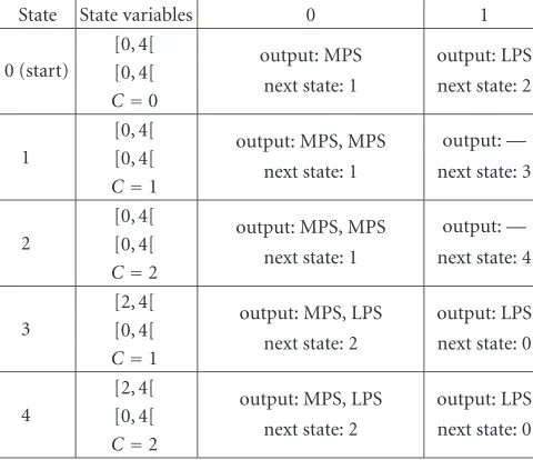
The state of the product system must gather state informa-tion of two automata: the automaton modeling the source distribution and the coder model. Hence, the stateX_kof the product system is defined as X_k = (lowS_k, upS_k,C_k). One could expect the dimension of the resulting state space to be the product of dimensions of the states spaces of the two models (source and coder). However, simplifications occur. Again, this is better explained with the simple source and coder examples ofTable 1andFigure 2.

The system resulting from the product of the coder of

Table 1 and the order-0 Markov source model ofFigure 2c

is illustrated inTable 3andFigure 4, respectively. ForT =4 and using the MPS/LPS simplification, the transitions do not lead to rescalings of the interval [lowS_k, upS_k[. For different values ofT, rescaling of the interval could occur and would then be signaled with the same notation f as inTable 1. Since the coder model has 2 states and the binary source model has 3 states, the dimension of the resulting state space should in principle be 6. However, it turns out that in general, fewer states are necessary (only 4 states instead of 6 in the sim-ple coder and source examsim-ples ofTable 1andFigure 2). This simplification results from the fact that the transitions in the coder model are a function of the source probability distribu-tion. Depending on the stationary probabilities of the input binary source, the general coder model given inTable 1 sim-plifies as shown inFigure 5. The probabilities of the binary symbols resulting from the conversion of theM-ary source depend on the previous state of the source model. Therefore, transitions on the source model will trigger the use of one of the two quasi-arithmetic trellis ofFigure 5. In the example of Figure 5b, it can be verified easily that some states will never be reached, hence reducing the state-space dimension from 6 to 4.

Table3: Source-coder product model: states, outputs, and transi-tions.

State State Variables MPS LPS

0 (start) [0, 4[ output: 0 output: 1

Figure4: Source-coder product model: trellis representation.

Xk=0 LPS (11)

Figure5: Quasi-arithmetic coder model: (a) 0.63≤P(MPS) and (b) 0.5≤P(MPS)<0.63.

In general, the state-space dimension cannot be known a priori; it must be computed, givenTand the binary source model. If NC is the number of states of the binary source model, the maximum number of states is 3T2_N

C/16. The number of bits produced by each transition on the above model being random, the structure of dependen-cies between the sequence of measurements and the model states is random. In order to capture this randomness, we actually consider the augmented Markov chain (X,N) =

S1 S2

Figure6: Source-coder product model (Nk≥Nk−1). White and black dots represent, respectively, the hidden and observed variables.

¯

Uk+1 = U_NN_kk+1+1 that have to be emitted and the next state

Xk+1. Notice that no bits may be emitted by a transition. The probabilities of successive branchings (e.g., of transitions be-tween (X_k,N_k)= (lowS_k, upS_k,C_k,N_k) and (X_k+1,Nk+1)= (lowS_k+1, upSk+1,Ck+1,Nk+1)) in the trellis are given by the binary source model, that is,P(Ck+1|Ck)=P(Sk+1|Ck). Mea-surements ¯Ykon the bits ¯Ukare gathered at the output of the transmission channel.

6.2. Product model: source and decoder

A product model of source and decoder can be con-structed similarly. The state of the product system must gather state information of the source and decoder mod-els. Hence, the stateX_nof the product system is defined as

Xn = (lowUn, upUn, lowSKn, upSKn,CKn). The system

re-sulting from the product of the decoder ofTable 2and the simple source model ofFigure 2cis illustrated inTable 4and Figure 7, respectively. Again, the state space dimension de-pends on the coder precision parametrized byTand of the source model.

The number of symbols being produced by each tran-sition on the above model is random. Therefore, the struc-ture of dependencies between the sequence of measure-ments and the sequence of decoded symbols is random. This is handled by considering the augmented Markov chain (X,K)=(X1,K1)· · ·(XN,KN) with the structure of depen-dencies graphically depicted inFigure 8. Using this model, a sequence of bitsU1N is translated into a sequence of sym-bolsSKN

1 , whereKNis the number of symbols decoded when

N bits have been received. Given a state X_n and an input bit Un+1, the automaton produces the sequence of symbols

¯

Sn+1=SK_Kn_n+1+1and the next stateXn+1. The probabilities of suc-cessive branchings (i.e., of transitions between (X_n,K_n) and (X_n+1,Kn+1)) in the trellis depend on the binary source model

Table4: Source-decoder product model: states, outputs, and tran-sitions.

State State variables 0 1

0 (start)

[0, 4[

output: MPS output: LPS [0, 4[

next state: 1 next state: 2

C=0

1

[0, 4[

output: MPS, MPS output: — [0, 4[

next state: 1 next state: 3

C=1

2

[0, 4[

output: MPS, MPS output: — [0, 4[

next state: 1 next state: 4

C=2

3

[2, 4[

output: MPS, LPS output: LPS [0, 4[

next state: 2 next state: 0

C=1

4

[2, 4[

output: MPS, LPS output: LPS [0, 4[

next state: 2 next state: 0

C=2

SK1

Figure8: Source-decoder product model. White and black dots represent, respectively, the hidden and observed variables.

6.3. Source distribution approximation

The entropy of the M-ary source computed on the binary

model inSection 6(e.g.,Figure 2c) is given by

HS|C= −NC

where C denotes the state variable of the source model, c the indices of the possible values it can take, andNCthe di-mension of the state space. The performance of the quasi-arithmetic coder when applied on this binary source for a given value of the parameterTcan be measured by

RS|X= −

where X denotes the state variable of the product model (source + coder),xrepresents the possible indices taken by the variable X, and N_X is the dimension of the state-space function ofT. The quasi-arithmetic coder realizes an approx-imation of the distribution of the binary source, hence of the

M-ary source. This approximation is, however, for a given value of the parameterT, more accurate than when apply-ing the quasi-arithmetic coder directly on theM-ary source. Here, the excess rate for a given value ofTis given by

ES|X=RS|X−HS|X between theapproximate conditional distributionQand the true conditional distributionP. One may notice that several states of the quasi-arithmetic coder can correspond to a given state cof the binary source model. Hence, several different approximationsQ(s|x) ofP(s|c) can exist (see, e.g., the states 0 and 3 ofTable 3). The excess rate can be considered as a measure of the bit stream redundancy.

7. ESTIMATION ALGORITHM

The above models of dependencies can be exploited to help the estimation of the bit stream (hence of the symbol se-quence). The MAP estimation criterion corresponds to the optimal Bayesian estimation of a processX, given available measurementsY:

However, if the mean square error (MSE) is the perfor-mance measure, the MAP criterion is suboptimal. The con-ditional mean or minimum MSE (MMSE) is in this case the optimal decoder. The decoder then seeks a sequence of symbol reproductions that will minimize the expected distortion, given the sequence of observations denoted by

E[D( ˆA,A)|Y]. These expected distortions can be computed in a very straightforward way, given the MAP estimates, pro-vided the probability measures on the sequence of binary symbolsSare converted into probability measures on the se-quence ofM-ary symbolsA. InSection 10, only the MAP es-timates have been considered.

The optimization is performed over all possiblesequences x. This applies directly to the estimation of the hidden states of the processes (X,N) (symbol-clock model of source + coder) and (X,K) (bit-clock model of source + decoder), given the sequence of measurements. The estimation is run on the source-decoder product model in order to avoid han-dling thenscl_kvariable.

Estimating the set of hidden states (X,K)=(X1,K1)· · · (XN,KN) is equivalent to estimating the associated sequence of decoded symbolsS = S1· · ·SKn· · ·SKN, given the

where ∝ denotes a renormalization factor. The Markov property allows a recursive computation of both terms of the right-hand side, using the BCJR algorithm [21]. The forward sweep concerns the first term

PXn=xn,Kn=kn|Y1n

The terms on the right-hand side of the equation are, re-spectively, the recursive term, the transition probability given by the product model (see Section 6), and the probability to have emitted the bitU_ntriggering the transition between

Xn−1 = xn−1andXn = xn, given the measureYn(channel model). The process is initialized at the starting state (0, 0) and allows to compute P(Xn,Kn|Y1n) for all possible states (x_n,k_n) and for each bit-clock instantn=1,. . .,N.

The backward sweep provides the second term in (10):

PYN

The process is initialized for all possible “last” states (x_N,k_N) and allows to computeP(Y_nN+1|Xn,Kn) for all possible states (x_n,k_n) and for each bit-clock instant consecutively fromN to 1.

As in [2,5], a termination constraint can be introduced; one can ensure that the decoder produces the right number of symbols (K_N =K) (if known). All the paths in the trellis which do not lead to a valid sequence length are suppressed. The trellis on which the estimation is performed can be pre-computed, with all transitions and outputs stored.Figure 9 shows the trellis computed with the example product model ofFigure 7for a sequence ofK=7 symbols producingN=

6 bits.

8. SOFT SYNCHRONIZATION

Termination constraints mentioned in Section 7can be re-garded as means to force synchronization at the end of the sequence; they indeed constrain the decoder to have the right number of symbols (K_N = K) (if known) after decoding the estimated bit stream ˆU. These constraints ensure syn-chronization at the end of the bit stream, but do not ensure synchronization in the middle of the sequence. One can in-troduce extra information specifically to help the resynchro-nization “in the middle” of the sequence. For this, we con-sider here the introduction of extra bits at some known

po-sitionsI_s = {i1,. . .,is}in the symbol stream. This extra in-formation takes the form of dummy binary symbols (in the spirit of the techniques described in [11,12,14,17,18]) in-serted in the binary symbol stream at some known symbol-clock positions after the conversion of theM-ary source into the binary source. Since these dummy symbols are inserted at some known symbol-clock instants, the position of the cor-responding extra bits in the coded bit stream depends on the sequence of symbols encoded, hence is random.

Models and algorithms above have to account for this ex-tra information. Inserting an exex-tra dummy symbol at known positions in the symbol stream amounts to add a section with deterministic transitions in the binary tree model of the source. The presence of this extra information can be ex-ploited by the estimation. During the estimation process, the variableK_nindicates when a marker should be expected. The corresponding transition probabilities in the estimation trel-lis are updated accordingly. A null probability is given to all transitions that do not emit the expected sequence of binary symbols, while a probability of one is set to the others. There-fore, some paths in the estimation trellis become forbidden and can be suppressed, leading to a reduction of the number of states.

9. ITERATIVE CC-AC DECODING ALGORITHM

The soft synchronization mechanism described above in-creases significantly the reliability of the segmentation and estimation of the sequence of symbols. One can however consider, in addition, the usage of an error correction code, for example, of a systematic convolutional CC. Both codes can be concatenated in the spirit of serial turbo codes. Adopt-ing this principle, one can therefore work on each model (quasi-arithmetic coder and channel coder) separately and design an iterative estimator, provided an interleaver is in-troduced between the models. The structure of dependencies between the variables involved is outlined inFigure 10.

Such a scheme requires extrinsic information on the bits

Unto be transmitted by the CC to the soft arithmetic decoder and reciprocally. The extrinsic information on a bitU_n rep-resents the modification induced by the introduction of the rest of the observationsYn−1

1 ,YnN+1on the conditional law of

UngivenYn. The extrinsic information can be expressed as

Ext_UnY|Yn∝ P

Un|Y

PUn|Yn. (13)

The iterative estimation proceeds by first running a BCJR al-gorithm on the channel coder model. The extrinsic informa-tion on the useful bitsU_nis a direct subproduct of the BCJR algorithm. These measurements can in turn be used as in-put for the estimation run on the quasi-arithmetic decoder model described above.

(0,0) 0

Figure10: Graphical representation of dependencies in the joint arithmetic-channel coding chain.

bitU_n =ungivenY is the sum of the transition probabili-ties between all states (xn−1,kn−1) and (xn,kn) for which this transition exists and is triggered byun. Thus, the a posteriori probability of a bitU_ngiven the observations is obtained by the equation

To evaluate the performance of the soft quasi-arithmetic decoding procedure, a set of experiments has been per-formed on a first-order Gauss-Markov source, with zero-mean, unit-variance, and different correlation factorsρ. The source is quantized with an eight-level uniform quantizer (3 bits) on the interval [−3, 3]. We consider sequences of

K = 200 symbols with different source correlation factors. All the simulations have been performed assuming an addi-tive white Gaussian channel with a binary phase shift keying (BPSK) modulation. The results are averaged over 3000 real-izations.

arithmetic codes [19], and quasi-arithmetic codes withT=4 for comparable overall rates. When the source correlation in-creases, the compression efficiency of the arithmetic coder increases; soft synchronization patterns are inserted in the arithmetically encoded stream up to a comparable overall rate. Figures11and12show the residual SERs and SNR ob-tained for different channelE_b/N0 for, respectively,ρ = 0.5 and ρ = 0.9. For sources with low correlation (ρ = 0.5 and under) and for values ofE_b/N0lower than 5 dB (i.e., for high bit error rates), quasi-arithmetic coding outperforms both arithmetic and Huffman coding. However, for sources with high correlation, the quasi-arithmetic coder and de-coder turn out to be slightly less efficient than the optimal arithmetic coder for this range ofEb/N0. The reason is that excess rate induced by quasi-arithmetic coding increases with the source correlation (see Section 4.3). The optimal arith-metic coding fully exploiting the source correlation, one can then insert a higher amount of soft synchronization pat-terns, for the same overall rate, resulting in an improved error resilience. The same trend has been observed for dif-ferent rates. The gain brought on soft quasi-arithmetic de-coding by synchronization markers is illustrated in Figures 13 and14, respectively, for ρ = 0.5 andρ = 0.9. Notice that, even for high correlation sources, the performances of the quasi-arithmetic decoder would obviously increase if one would allow a higher complexity, that is, a higher value for the parameterT. In order to compare fairly the three meth-ods, one must also consider their complexity. It can be mea-sured by the size of the trellis used for the estimation. Con-sidering a sequence of 200 symbols, soft decoding of Huff -man codes needs two trellises with about 900 states, respec-tively, per bit-clock and symbol-clock instants. The complex-ity of soft decoding of arithmetic codes is limited to 100 states per symbol-clock instant, using pruning. Finally, the soft de-coding of quasi-arithmetic codes leads to a trellis containing about 2400 states per bit-clock instant, hence being the most complex of the three. Pruning may be considered to reduce this complexity.

The second experiment aimed at evaluating the perfor-mance of the iterative channel/quasi-arithmetic decoding al-gorithm. Figures 15 and16 depict the SER and SNR per-formances in comparison with the decoding approach with soft synchronization, respectively, forρ = 0.5 andρ =0.9. The first observation is that the iterations bring significant improvements and higher gain is being obtained when the source correlation is high (seeFigure 16). Nevertheless, if the source correlation is low, the soft synchronization outper-forms the iterative scheme. In this range of channel SNRs, the CC cannot correct all the errors, and the desynchro-nization phenomenon prevails. It is therefore preferable to dedicate redundancy within the source to fight against these desynchronizations. In contrast, when the source correlation is high (ρ = 0.9), the SER is lower with the iterative solu-tion due to a proper exploitasolu-tion of the intersymbol corre-lation for segmenting and estimating the bit stream. It can also be observed that the gain brought by the iterations de-pends on the degree of redundancy present on both sides of

the interleaver. Figures17and18show the performances ob-tained when combining synchronization markers and chan-nel coding, respectively, forρ=0.5 andρ =0.9. Three ap-proaches are compared, with equal or sufficiently close over-all rates. In the first one, only channel coding (k/n = 2/3 and 4 iterations) is used to add redundancy. In the second one, channel coding (k/n = 5/6 and 4 iterations) is com-bined with synchronization markers. Finally, in the third ap-proach, only synchronization markers are used. For sources with high correlation, channel coding leads to higher per-formance since the correlation present in the source is al-ready exploited efficiently to fight against desynchroniza-tions. For sources with low correlation and for values of

Eb/N0 lower than 3 dB, on the contrary, the combination of channel coding and synchronization markers has been found to be the best strategy. It has also been observed that, in this case, iterations bring a higher gain than in other cases.

In another set of experiments, the influence of the length of the sequence on the system performance is considered. Figures 19 and20 depict the SER and SNR performances with three different lengths, respectively, for ρ = 0.5 and

ρ = 0.9. As expected, the performance decreases when the length of the sequence increases. This can be explained by the exploitation of the termination constraint which con-tributes to the decoder resynchronization. The length of the sequence has also an influence on the complexity of the de-coding. Indeed, this complexity depends on the size of the es-timated trellis, which depends mainly on theexcursion, that is, the possible values, of the variable K_n. The excursion is higher in the middle than at the extremities of the sequence. Hence, it reaches higher values with longer sequences. We have measured experimentally the average number of states of the trellis per bit-clock instantn. The values obtained are 557, 1177, and 2376, respectively, for sequences of 50, 100, and 200 symbols. Pruning techniques may be required for longer sequences.

100

10−1

10−2

10−3

10−4

SER

0 2 4 6

Eb/N0

Soft Huffman 2.53 bpss Soft arithmatic 2.53 bpss SoftQ-arithmatic 2.53 bpss

(a) 50

45 40 35 30 25 20 15 10 5

SNR

0 2 4 6

Eb/N0

Soft Huffman 2.53 bpss Soft arithmatic 2.53 bpss SoftQ-arithmatic 2.53 bpss

(b)

Figure11: SER and SNR performances of (i) soft Huffman decod-ing, (ii) soft arithmetic decoddecod-ing, and (iii) soft quasi-arithmetic de-coding (ρ=0.5, 200 symbols, 3000 channel realizations).

100

10−1

10−2

10−3

10−4

SER

0 2 4 6

Eb/N0

Soft Huffman 2.53 bpss Soft arithmatic 2.43 bpss SoftQ-arithmatic 2.43 bpss

(a)

45

40

35

30

25

20

15

10

SNR

0 2 4 6

Eb/N0

Soft Huffman 2.53 bpss Soft arithmatic 2.43 bpss SoftQ-arithmatic 2.43 bpss

(b)

100

10−1

10−2

10−3

SER

0 2 4 6

Eb/N0

SoftQ-arithmatic 2.43 bpss SoftQ-arithmatic 2.53 bpss SoftQ-arithmatic 2.73 bpss

(a)

35

30

25

20

15

10

5

SNR

0 2 4 6

Eb/N0

SoftQ-arithmatic 2.43 bpss SoftQ-arithmatic 2.53 bpss SoftQ-arithmatic 2.73 bpss

(b)

Figure13: SER and SNR performances of soft quasi-arithmetic de-coding for different rates (ρ=0.5, 200 symbols, 3000 channel real-izations).

100

10−1

10−2

10−3

10−4

SER

0 2 4 6

Eb/N0

SoftQ-arithmatic 2.02 bpss SoftQ-arithmatic 2.53 bpss SoftQ-arithmatic 2.73 bpss

(a)

45

40

35

30

25

20

15

10

SNR

0 2 4 6

Eb/N0

SoftQ-arithmatic 2.02 bpss SoftQ-arithmatic 2.53 bpss SoftQ-arithmatic 2.73 bpss

(b)

100

10−1

10−2

10−3

10−4

SER

0 2 4 6

Eb/N0

Soft_Q-arithmatic 2_.91 bpss

SoftQ-arithmatic + CC 2.90 bpss, iteration 1 SoftQ-arithmatic + CC 2.90 bpss, iteration 4

(a) 50

45 40 35 30 25 20 15 10 5

SNR

0 2 4 6

Eb/N0

SoftQ-arithmatic 2.91 bpss

SoftQ-arithmatic + CC 2.90 bpss, iteration 1 SoftQ-arithmatic + CC 2.90 bpss, iteration 4

(b)

Figure15: SER and SNR performances of (i) soft quasi-arithmetic decoding with soft synchronization and (ii) turbo quasi-arithmetic/ channel decoding (ρ=0.5, 200 symbols, 3000 channel realizations).

100

10−1

10−2

10−3

10−4

10−5

SER

0 2 4 6

Eb/N0

Soft_Q-arithmatic 2_.69 bpss

SoftQ-arithmatic + CC 2.69 bpss, iteration 1 SoftQ-arithmatic + CC 2.69 bpss, iteration 4

(a) 50

45

40

35

30

25

20

15

SNR

0 2 4 6

Eb/N0

SoftQ-arithmatic 2.69 bpss

Soft_Q-arithmatic + CC 2_.69 bpss, iteration 1 SoftQ-arithmatic + CC 2.69 bpss, iteration 4

(b)

100

10−1

10−2

10−3

10−4

SER

0 1 2 3 4

Eb/N0

SoftQ-arithmatic + CC 3.65 bpss SoftQ-arithmatic + CC + M 3.65 bpss SoftQ-arithmatic + M 3.65 bpss

(a) 50

45 40 35 30 25 20 15 10

SNR

0 1 2 3 4

Eb/N0

SoftQ-arithmatic + CC 3.65 bpss SoftQ-arithmatic + CC + M 3.65 bpss SoftQ-arithmatic + M 3.65 bpss

(b)

Figure 17: SER and SNR performances of (i) turbo quasi-arithmetic/channel decoding, (ii) turbo quasi-quasi-arithmetic/channel decoding with soft synchronization, and (iii) soft quasi-arithmetic decoding with soft synchronization (ρ = 0.5, 200 symbols, 1500 channel realizations).

10−1

10−2

10−3

10−4

10−5

SER

0 1 2 3 4

Eb/N0

Soft_Q-arithmatic + CC 3_.10 bpss SoftQ-arithmatic + CC + M 3.25 bpss SoftQ-arithmatic + M 3.21 bpss

(a) 55

50

45

40

35

30

25

20

SNR

0 1 2 3 4

Eb/N0

SoftQ-arithmatic + CC 3.10 bpss SoftQ-arithmatic + CC + M 3.25 bpss SoftQ-arithmatic + M 3.21 bpss

(b)

100

10−1

10−2

SER

0 1 2 3 4

Eb/N0

Soft_Q-arithmatic 50 symbols SoftQ-arithmatic 100 symbols SoftQ-arithmatic 200 symbols

(a)

22

20

18

16

14

12

10

SNR

0 1 2 3 4

Eb/N0

SoftQ-arithmatic 50 symbols SoftQ-arithmatic 100 symbols SoftQ-arithmatic 200 symbols

(b)

Figure19: SER and SNR performances of soft quasi-arithmetic de-coding for, respectively, 50, 100, and 200 symbols (ρ =0.5, 3000 channel realizations).

100

10−1

10−2

10−3

SER

0 1 2 3 4

Eb/N0

Soft_Q-arithmatic 50 symbols SoftQ-arithmatic 100 symbols SoftQ-arithmatic 200 symbols

(a)

34 32 30 28 26 24 22 20 18 16

SNR

0 1 2 3 4

Eb/N0

SoftQ-arithmatic 50 symbols SoftQ-arithmatic 100 symbols SoftQ-arithmatic 200 symbols

(b)

100

10−1

10−2

10−3

SER

0 2 4 6

Eb/N0

T=4 2.43 bpss

T=8 2.30 bpss

T=8 2.43 bpss (a) 30

25

20

15

10

5

SNR

0 2 4 6

Eb/N0

T=4 2.43 bpss

T=8 2.30 bpss

T=8 2.43 bpss (b)

Figure21: SER and SNR performances of (i) soft quasi-arithmetic decoding (T=4), (ii) soft quasi-arithmetic decoding (T=8), and (iii) soft quasi-arithmetic decoding (T=8) with soft synchroniza-tion (ρ=0.5, 100 symbols, 3000 channel realizations).

11. CONCLUSION

Arithmetic codes are becoming more and more popular in practical compression systems and emerging standards. Their well-known drawback is however their very high sen-sitivity to noise. MAP estimators running on the coding tree can help to fight against errors and possible decoder desynchronization but at the expense of rather high com-plexity. The coding tree grows exponentially with the num-ber of symbols in the sequence to be coded. Here, we have considered an alternate solution based on reduced-precision arithmetic codes, called arithmetic codes. A quasi-arithmetic coder can be viewed as a finite-state stochastic automaton. One can then run MAP estimators on the re-sulting model. For the sake of clarity, we have considered simple source models in the examples. The results reported have been obtained considering an order-1 Markov source. However, the approach extends very easily to higher-order source models. The state model of the coding and decod-ing process is of finite size. Its size depends on the accept-able approximation of the source distribution. The decod-ing complexity remains within a realistic range without the need for applying any pruning. Placed in an iterative de-coding structure in the spirit of serially concatenated turbo codes, the estimation process can then benefit from the iter-ations. Overall, the flexibility they offer for adjusting com-pression efficiency, complexity, and error resilience allows an optimal adaptation to various transmission conditions and terminal capabilities. Notice that, for low complexity, a very good trade-offcompression-noise resilience can be achieved with quasi-arithmetic codes for low correlation sources. This emphasizes the interest of the above solution for practical systems, where the coder is applied on quantized decorre-lated sequences of symbols.

REFERENCES

[1] K. P. Subbalakshmi and J. Vaisey, “On the joint source-channel decoding of variable-length encoded sources: the BSC case,”IEEE Trans. Communications, vol. 49, no. 12, pp. 2052– 2055, 2001.

[2] M. Park and D. J. Miller, “Joint source-channel decoding for variable-length encoded data by exact and approximate MAP sequence estimation,” IEEE Trans. Communications, vol. 48, no. 1, pp. 1–6, 2000.

[3] M. Park and D. J. Miller, “Decoding entropy-coded symbols over noisy channels by MAP sequence estimation for asyn-chronous HMMs,” inProc. Annual Conference on Information Sciences and Systems (CISS ’98), pp. 477–482, Princeton, NJ, USA, March 1998.

[4] A. H. Murad and T. E. Fuja, “Joint source-channel decoding of variable length encoded sources,” inProc. Information Theory Workshop (ITW ’98), pp. 94–95, Killarney, Ireland, June 1998. [5] N. Demir and K. Sayood, “Joint source/channel coding for variable length codes,” inProc. IEEE Data Compression Conference (DCC ’98), pp. 139–148, Snowbird, Utah, USA, March–April 1998.

[6] R. Bauer and J. Hagenauer, “Turbo FEC/VLC decoding and its application to text compression,” inProc. 34th Annual Confer-ence on Information SciConfer-ences and Systems (CISS ’00), pp. WA6– WA11, Princeton, NJ, USA, March 2000.

source-channel turbo decoding of entropy-coded sources,”

IEEE Journal on Selected Areas in Communications, vol. 19, no. 9, pp. 1680–1696, 2001.

[8] R. Bauer and J. Hagenauer, “Iterative source/channel decod-ing based on a trellis representation for variable length codes,” inProc. IEEE International Symposium on Information Theory (ISIT ’00), p. 117, Sorrento, Italy, June 2000.

[9] Y. Takishima, M. Wada, and H. Murakami, “Reversible vari-able length codes,” IEEE Trans. Communications, vol. 43, no. 4, pp. 158–162, 1995.

[10] J. Wen and J. D. Villasenor, “Reversible variable length codes for efficient and robust image and video coding,” inProc. IEEE Data Compression Conference (DCC ’98), pp. 471–480, Snow-bird, Utah, USA, March–April 1998.

[11] G. F. Elmasry, “Embedding channel coding in arithmetic cod-ing,”IEE Proceedings-Communications, vol. 146, no. 2, pp. 73– 78, 1999.

[12] C. Boyd, J. G. Cleary, S. A. Irvine, I. Rinsma-Melchert, and I. H. Witten, “Integrating error detection into arithmetic cod-ing,” IEEE Trans. Communications, vol. 45, no. 1, pp. 1–3, 1997.

[13] G. F. Elmasry, “Joint lossless-source and channel coding using automatic repeat request,” IEEE Trans. Communications, vol. 47, no. 7, pp. 953–955, 1999.

[14] I. Sodagar, B. B. Chai, and J. Wus, “A new error resilience technique for image compression using arithmetic coding,” inProc. IEEE Int. Conf. Acoustics, Speech, Signal Processing (ICASSP ’00), pp. 2127–2130, Istanbul, Turkey, June 2000. [15] J. Chou and K. Ramchandran, “Arithmetic coding-based

con-tinuous error detection for efficient ARQ-based image trans-mission,” IEEE Journal on Selected Areas in Communications, vol. 18, no. 6, pp. 861–867, 2000.

[16] I. Kozintsev, J. Chou, and K. Ramchandran, “Image transmis-sion using arithmetic coding based continuous error detec-tion,” inProc. IEEE Data Compression Conference (DCC ’98), pp. 339–348, Snowbird, Utah, USA, March–April 1998. [17] B. D. Pettijohn, M. W. Hoffman, and K. Sayood, “Joint

source/channel coding using arithmetic codes,” IEEE Trans. Communications, vol. 49, no. 5, pp. 826–836, 2001. [18] C. Demiroglu, M. W. Hoffman, and K. Sayood, “Joint source

channel coding using arithmetic codes and trellis coded mod-ulation,” inProc. 11th IEEE Data Compression Conference (DCC ’01), pp. 302–311, Snowbird, Utah, USA, March 2001. [19] T. Guionnet and C. Guillemot, “Soft decoding and

synchro-nization of arithmetic codes: application to image transmis-sion over noisy channels,” IEEE Trans. Image Processing, vol. 12, no. 12, pp. 1599–1609, 2003.

[20] P. G. Howard and J. S. Vitter, “Practical implementations of arithmetic coding,” inImage and Text Compression, pp. 85– 112, Kluwer Academic, Norwell, Mass, USA, 1992.

[21] L. R. Bahl, J. Cocke, F. Jelinek, and J. Raviv, “Optimal decoding of linear codes for minimizing symbol error rate,”IEEE Trans-actions on Information Theory, vol. 20, pp. 284–287, March 1974.

[22] J. J. Rissanen, “Generalized Kraft inequality and arithmetic coding,” IBM Journal of Research and Development, vol. 20, no. 3, pp. 198–203, 1976.

[23] R. Pasco, Source coding algorithms for fast data compression, Ph.D. thesis, Department of Electrical Engineering, Stanford University, Stanford, Calif, USA, 1976.

[24] J. J. Rissanen, “Arithmetic codings as number representa-tions,”Acta Polytechnica Scandinavica, vol. 31, pp. 44–51, De-cember 1979.

[25] I. H. Witten, R. M. Neal, and J. G. Cleary, “Arithmetic coding for data compression,” Communications of the ACM, vol. 30, no. 6, pp. 520–540, 1987.

[26] P. G. Howard and J. S. Vitter, “Design and analysis of fast text compression based on quasi-arithmetic coding,” inProc. IEEE Data Compression Conference (DCC ’93), pp. 98–107, Snow-bird, Utah, USA, March–April 1993.

Thomas Guionnet received his B.S. de-gree from the University of Newcastle Upon Tyne, UK, in computer science in 1997. He obtained the Engineer Degree in computer science and image processing and the Ph.D. degree from the University of Rennes 1, France, respectively, in 1999 and 2003. He is currently a Research Engineer at INRIA and is involved in the French national project RNRT VIP and in the JPEG 2000 Part

11-JPWL ad hoc group. His research interests include image process-ing, codprocess-ing, and joint source and channel coding.

Christine Guillemotis currently “Directeur de Recherche” at INRIA, in charge of a re-search group dealing with image modelling, processing, and video communication. She holds a Ph.D. degree from ´Ecole Na-tionale Sup´erieure des T´el´ecommunications (ENST) Paris. Her research interests are sig-nal and image processing, coding, and joint source and channel coding. From 1985 to October 1997, she has been with France