R E S E A R C H
Open Access
A novel sequential algorithm for clutter
and direct signal cancellation in passive
bistatic radars
Farzad Ansari
1, Mohammad Reza Taban
2*and Saeed Gazor
3Abstract
Cancellation of clutter and multipath is an important problem in passive bistatic radars. Some important recent algorithms such as the ECA, the SCA and the ECA-B project the received signals onto a subspace orthogonal to both clutter and pre-detected target subspaces. In this paper, we generalize the SCA algorithm and propose a novel sequential algorithm for clutter and multipath cancellation in the passive radars. This proposed sequential
cancellation batch (SCB) algorithm has lower complexity and requires less memory than the mentioned methods. The SCB algorithm can be employed for static and non-static clutter cancellation. The proposed algorithm is evaluated by computer simulation under practical FM radio signals. Simulation results reveal that the SCB provides an admissible performance with lower computational complexity.
Keywords: Passive radar, Bistatic multipath, Clutter cancellation
1 Introduction
Passive bistatic radars use the reflected signals from independent transmitters as illuminators of opportunity. Passive radars stay hidden and cannot be identified or localized as they do not transmit signals while they detect aerial targets. In this type of radar, the utilized signals can be analogue TV [1, 2], FM radio [3], satellite [4], DVB-T [5], DAB [6] and GSM [7] which may be present in the space and can be treated as the transmitted signal. In gen-eral, the selection of suitable illumination signals depends on some parameters such as the coverage area of these transmitters, their power and their carrier frequency and bandwidth. Commercial FM radio stations are one of the best available signal sources which yield good perfor-mance for this purpose along with low implementation costs [3]. In particular, the high transmit powers of FM broadcast stations often allow detection ranges of approx-imately 250 km [8]. Figure 1 illustrates a common scenario that often occurs in the passive radars, where the passive radar is equipped with a receive reference antenna and a surveillance antenna.
*Correspondence: [email protected]
2Department of Electrical and Computer Engineering, Isfahan University of
Technology, Isfahan 84156-83111, Iran
Full list of author information is available at the end of the article
The reference antenna is adjusted to receive only the direct path of the signal from the transmitter, while the surveillance antenna receives signals from all directions which includes signals not only from the direct path from the FM station but also from the reflections produced by targets and clutters. Using the ambiguity function based on the matched filters [3, 9], the Range-Doppler targets and clutter are detectable.
Before computing the ambiguity function, there are some challenges that must be resolved. For example, the power of the direct path signal is significantly higher than the received power from targets, and the signal received from the target and clutter often go through multipath unknown channels. Various methods have been proposed to confront these problems. Some of them have consid-ered the problem as a composite hypothesis test and have attempted to design sub-optimal detectors such as gen-eralized likelihood ratio test for target detection in the presence of the interference [10, 11]. Some others have employed adaptive filters to estimate the clutter and direct path signal components in order to cancel them [12, 13]. However, an important class of methods is based on the projection of the received signal onto a subspace orthog-onal to both the clutter and the pre-detected targets. The ECA, SCA and ECA-B are among these methods [14–16].
Fig. 1A common scenario of passive radars
Recently, a version of ECA (ECA-S) has been proposed in [17].
In this paper, we propose a novel algorithm for clut-ter and multipath cancellation for the passive radars by generalization of some recent algorithms which we call as the sequential cancellation batch (SCB) algorithm. Our simulation results show that the proposed SCB outper-forms or peroutper-forms as good as the mentioned state-of-the-art methods, depending on the conditions. Furthermore, the proposed SCB requires lesser memory than these existing state-of-the-art methods. Our simulations show that after clutter and direct signal cancellation using the SCB algorithm, weak targets likely are not detectable. Hence, in this paper, we use CLEAN algorithm [18–20] for weak target detection. Although in this paper, we con-centrate on the use of commercial FM radio signals, it should be noted that the proposed method (SCB) can be applied to any transmission of opportunity, such as GSM transmissions, DAB or DVB-T and satellites. Indeed, the choice of FM transmissions arguably results in wave-forms with the worst ambiguity properties for target detection.
The paper is organized as follows. Section 2 presents the signal model and ambiguity function. Section 3 introduces the ECA and SCA algorithms and describes the proposed SCB technique, and in Section 4, three tests are intro-duced for comparison of the performance of algorithms. Finally, Section 5 is our conclusions.
Notations: Throughout this paper, we use boldface lower case and capital letters to denote vector and matrix, respectively. We useO(.)as the complexity order of algo-rithms.diag(.,. . ., .)denotes diagonal matrix containing the elements on the main diameter.0N×Ris anN×Rzero
matrix andINis anN×Nidentical matrix. Also(.)T,(.)∗
and(.)H stand for the transpose, conjugate and Hermi-tian of a matrix or vector, respectively. The operator . denotes the integer part (or floor) of a number.
2 Signal model and ambiguity function
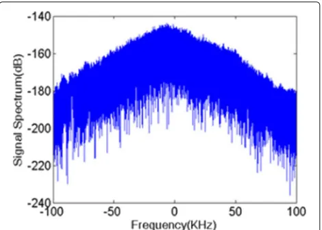
The FM radio signals used in passive radar are in the 88- to 108-MHz band. For example, in Fig. 2, the spec-trum of a commercial FM signal is showed that is used for simulation scenario.
Fig. 2Spectrum of FM signal used for simulated scenario
As seen in Fig. 1, two required signals are used for inter-ference cancellation algorithms. One is the main received signal from the surveillance antenna and another is an auxiliary signal yielded from the reference antenna. IfTint is the duration time of signal observation, the received signalssur(t)at the surveillance antenna is modelled as:
ssur(t)=Asurd(t)+
where d(t)is the direct transmitted signal that is multi-plied by the complex amplitude Asur. The variablesam,
τmandfdmare the complex amplitude, delay and Doppler
frequency of the mth target signal (m = 1,. . .,NT),
respectively, that isNT is the number of targets.ci(t)and
τciare the complex amplitude function and delay of theith
clutter (i=1,. . .,NC), that isNCis the number of clutters.
All delays are calculated with respect to the direct signal. nsur(t) is the thermal noise contribution at the receiver antenna.
The complex amplitudes ci(t) are considered slowly
varying functions of time, so that they can be repre-sented by only a few frequency components around zero Doppler:
ci(t)=ciej2πfcit, (2)
wherefciandciare Doppler shift and complex amplitude
of theith clutter (i=1,. . .,NC), respectively. In the same
way, the received signalsref(t)at the reference antenna is:
sref(t)=Arefd(t)+nref(t), (3)
The samples collected at the surveillance channel at the time instants tn = nTs, (n = 0, 1,. . .,N − 1)
are arranged in a N × 1 vector ssur, where Ts is the
sampling time and N is the number of samples to be integrated. The sampling time is selected greater than the resolution time (i.e. Ts > 1/B where B is the
sys-tem bandwidth). Similarly, we collectN +Rsamples of the signal at the reference channel in a (N + R) × 1 vector sref. We use the ambiguity function for evalua-tion of the interference cancellaevalua-tion algorithms and target detection. The discrete ambiguity function equation is as follows [9]:
tively. Consider that the discrete delaylcorresponds to the delayT[l]= lTs andRis maximum delay bin of clutter.
Similarly, the discrete Doppler frequency bin p, corre-sponds to the Doppler frequencyfd[p]=p/(NTs)andPis
maximum Doppler bin of clutter.
3 Clutter and direct signal cancellation
In this section, first we introduce two known algorithms ECA and SCA for clutter and direct signal cancellation in passive bistatic radars. Then the proposed algorithm is presented.
3.1 Extensive cancellation algorithm (ECA)
The ECA is an effective way for clutter and direct signal cancellation in the passive radars and is based on the least-squares (LS) estimation [14]. If the surveillance vectorssur is modelled with respect to the reference vectorsref lin-early, the objective function in the LS estimation can be represented as follows:
min
θ ssur−Hθ , (5)
whereθis the model parameters vector corresponding to the likely clutters andHis a known matrix depending on the positive integerpas:
H=B[-psref . . .-1sref sref 1sref . . . psref] . (6)
Here,Bis an incidence matrix that selects only the last N rows of the next multiplied matrix and has the below form:
B=[0N×R...IN]. (7)
p is a diagonal matrix making the phase shift
corre-sponding to thepth Doppler bin, as:
p=diag
1,ej2πpTs,. . .,ej2π(N+R−1)pTs. (8) Also,sref=[sref Dsref D2sref . . . Dk−1sref], whereD is a 0/1 permutation matrix that imposes a delay unit to the next multiplied vector andkindicates the maximum amount of delay in clutter samples. Indeed, the columns of srefare the delayed versions of the zero-Doppler reference signal. The columns of matrixHpresent a basis for the M-dimensional clutter subspace, whereM = (2p+1)k. The solution of (7) yieldsθˆ = (HHH)-1HHs
sur; therefore, the received signal after cancellation of direct signal and clutter can be obtained as:
sECA =ssur−Hθˆ=(IN−H(H
H
H)-1HH)ssur=P0ssur.
(9)
The computational complexity of the ECA algorithm is O(NM2+M3). This complexity is high because the esti-mation of vector θ requires the inversion of the matrix HHHwith dimensionsM×M.
3.2 Sequential cancellation algorithm (SCA)
Aiming at reducing the computational load of the ECA algorithm described in Section 3.1, a sequential solution algorithm has been offered in [14] for clutter and direct signal cancellation, called SCA.
Consider the matrixH=[x0x1 · · · xM−1], wherexiis
the(i+1)th column ofH. The sequential equations of the SCA algorithm are as follows:
• Start with initial equations as:
PM=IN, (10)
¯
s(surM)=ssur. (11) • Then, the output vector of SCA algorithm is obtained
by implementing the below recursive equations for i=M,. . ., 2, 1respectively: • In each step of the above equations, the received
signal can be improved one level as:
s(suri-1)=Pi-1ssur =Qis(suri). (15) • After finishing the above loop, by using the final
projection matrixP0, the output vectorsSCAis obtained as follows:
A schematic plan of the SCA algorithm containing the clutter and direct signal cancellation is shown in Fig. 3.
Almost all steps of a SCA algorithm have been shown in this figure. It is possible to limit the computational of the cancellation algorithm by arresting it after stageS (S < M). The computational complexity of the SCA algorithm limited toSstage isO(NMS), which can be significantly smaller than the computational cost of the corresponding complete ECA algorithm.
3.3 Sequential cancellation batch (SCB) algorithm
In order to improve the cancellation performance with a limited computational load, a modification of the SCA is proposed which is called SCB. The received signal at the surveillance antenna is divided into sections with length TB. If the entire length of the surveillance antenna
sig-nal is Tint, the total number of samples of the signal at the antenna will beN = Tintfs, where fs is the
sam-pling frequency. The signal is divided intobpackets with NB = N/b available samples. First, the SCA
algo-rithm is applied to each of these packets distinctly. The output of the SCA algorithm on each packet is a vec-tor removed of the clutter and direct signal. Then, the
main cleaned vector is obtained from the union of these sub-vectors. Finally, the main vector can be used for com-puting and plotting the ambiguity diagram and target detection.
In this manner, vectors ssurv(j) and sref(j)
correspond-ing to the(j+1)th packet are defined as follows forj = 0, 1, 2,. . .,b−1
ssurv(j)=ssur
jNB
ssur
jNB+1
. . .ssur
(j+1)NB−1
T , (17)
sref(j)=
sref
jNB-R
sref
jNB-R+1
. . .ssur(j+1)NB−1
T . (18)
If the output of the SCA algorithm on the jth packet denotes vectorsSCA(j), the total outputsSCBremoved from the clutter and direct signal is obtained as:
sSCB= sTSCA(0) sTSCA(1) . . . sTSCA(b−1)
T
. (19)
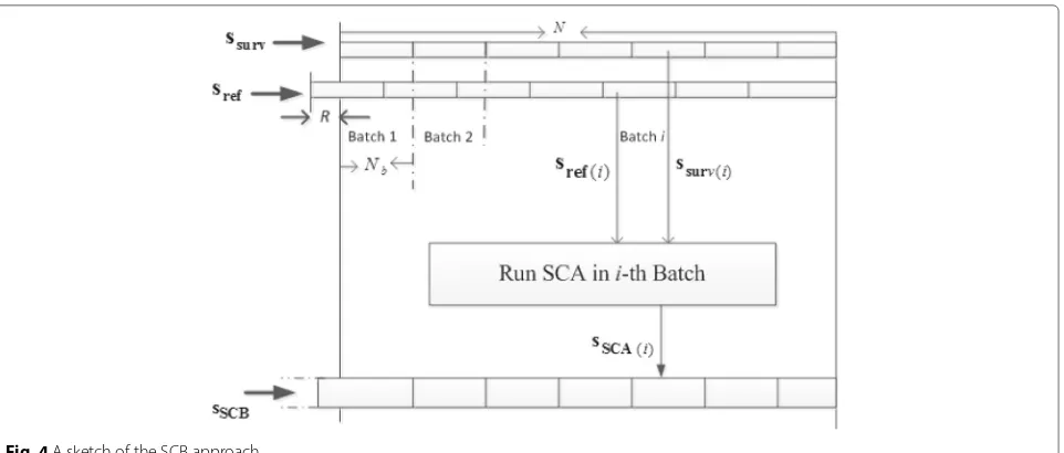
A schematic plan of the SCB algorithm is shown in Fig. 4. If we replace the applied SCA method with ECA
Fig. 4A sketch of the SCB approach
method in the SCB algorithm (instead of the SCA block that runs on theith batch in the block diagram of Fig. 4), the ECA-B method will be achieved which is explained in [15] fully.
We use the observation or CLEAN algorithm [18–21] for detection of the weak target. The Doppler frequency
(fˆi1), delay(τˆi1)and amplitude(Aˆi1)of theith strong target
(i = 1,. . .,Ns1) can be extracted based on the infor-mation of location of this strong target in the ambiguity function whereNs1is the number of strong targets which are detected after SCB algorithms. Then, the estimated echoes of the strong targets are subtracted fromsSCB(t)as follows:
s1sur(t)=sSCB(t)− Ns1
i=1 ˆ
Ai1d(t− ˆτi1)e2πjfˆi1t, (20)
where sSCB(t) is the signal removed from clutter
and direct signal by the SCB algorithm. By comput-ing the ambiguity function of s1
sur(t), the weak tar-gets can appear. In the next processing, the estimated echoes of new targets (the weak targets in ambigu-ity function of s1sur(t)) are subtracted from s1sur(t) as follows:
s2sur(t)=s1sur(t)−
Ns2
i=1 ˆ Ai2d
t− ˆτi2
e2πjˆfi2t. (21)
Here, the Doppler frequency(fˆi2), delay(τˆi2)and ampli-tude (Aˆi2) of each weak target can be extracted based on the information of location of these weak targets in the ambiguity function ofs1sur(t), andNs2is the number
of weak targets which are detected in ambiguity func-tion ofs1sur(t). The observation algorithm is repeated as follows:
sjsur(t)=sjsur−1(t)−
Nsj
i=1 ˆ
Aijd(t− ˆτij)e2πjfˆijt, j=2, 3,. . .
(22)
where ˆfij, τˆij and Aˆij are the the Doppler frequency,
delay and amplitude of unregarded weak targets which appeared in the (j− 1)th stage and detected using the ambiguity function of sjsur−1(t). The algorithm is ended when the below inequality occurs:
maxξτd,fd
−minξτd,fd
maxξτd,fd
< η, (23)
whereξ(τd,fd)is the ambiguity function ofsjsur(t)at posi-tion(τd,fd)andηis a small value selected between zero
and one in our simulations.
The computational complexity of the SCB algorithm in each batch isO(NBMS). This means that the SCB
algo-rithm requires lesser memory than the ECA and SCA algorithms. When the SCB algorithm is run onbbatches, the computational complexity will beO(bNBMS)which is
equal to the SCA algorithm becausebNBequalsN.
We remind that the computational complexity of ECA-B method isONM2+M3similar to the ECA method; but its required memory isONBM2+M3
4 Results and discussion
In this section, we investigate the performance of the pro-posed algorithm and compare it with the ECA, SCA and ECA-B methods. For this purpose, we use two different Doppler-delay scenarios. First, in scenario #1 represented in Fig. 5, we consider nine clutters in the form of blue stars and three targets in the form of red circles.
The clutter and target specifications are shown in Tables 1 and 2, respectively. Also, the signal-to-noise ratio (SNR) of the direct signal is assumed to be 60 dB.
Figure 6 shows the ambiguity function of the received signal in scenario #1, in a two-dimensional (2-D) mode without removing the direct signal and clutter. In Fig. 6a, it is seen that the peaks of targets are masked by the peaks of direct signal and clutters, and the targets are not dis-tinguishable. In Fig. 6b, the output of ambiguity function is drawn for l = 0. In this figure, the strong peak cor-responding to the direct signal (with zero Doppler and zero delay) is presented obviously. The output of ambi-guity function for p = 0 is also presented in Fig. 6c. In this figure, it is shown that the clutter is delayed up to 0.25 ms, and most of the amounts of ambigu-ity function are in zero delay, indicating the direct path signal.
First, we implement the ECA algorithm under scenario #1. Figure 7a shows the 2-D ambiguity function of the received signal after the direct signal and all echoes of clutter cancellation by the ECA algorithm. The simulation conditions arek= 50 and Doppler bin(−1, 0, 1), wherep is 1. As seen in Fig. 7a, the two strong targets now appear, but the weak target is still not detectable. Figure 7b shows the ambiguity function versus delay in Doppler shiftl=0.
Fig. 5Representation of scenario #1
Table 1Clutter echo parameters in scenario #1
Clutter #1 #2 #3 #4 #5 #6 #7 #8 #9
Delay (ms) 0.05 0.1 0.15 0.2 0.25 0.1 0.17 0.22 0.25
Doppler (Hz) 0 0 0 0 0 1 1 1 1
CNR (dB) 40 30 20 10 5 27 18 8 5
This figure shows that the direct signal and all clutters cor-responding to the delays inside the firstkbins have been removed.
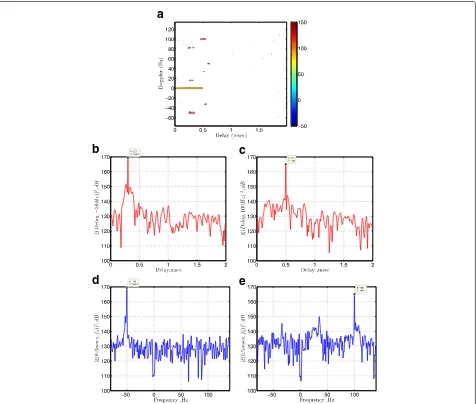
Then, the SCB algorithm is simulated based on sce-nario #1. The information required for the simulation is shown in Table 3. Figure 8a shows the 2-D ambigu-ity function of the received signal after cancelling all the clutters and direct signal using the SCB algorithm. This simulation has been prepared withS= 100, Doppler bin
(−1, 0, 1)andk = 50. The cancellation of the direct sig-nal and clutter causes the strong targets to be seen better, and by using a simple detector such as the cell-averaging constant false-alarm rate (CA-CFAR), they can simply be detected. Nonetheless, the weak target has not been detected. Figure 8b, c shows the ambiguity function ver-sus delay for Doppler shifts−50 and 100 Hz, and Fig. 8d, e shows the ambiguity function versus Doppler for delays 0.3 and 0.5 ms, respectively. In these four figures, it is seen that unlike the weak targets, the locations of two strong targets are shown obviously.
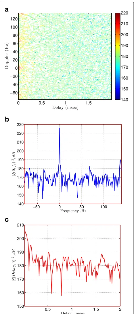
For illustrating the modified SCB method equipped with CLEAN technique, Fig. 9a shows the 2-D ambigu-ity function output of received signal after removing the direct signal and all the clutters by the SCB algorithm, and the strongest target using the observation algorithm (consider that Fig. 9 presents the ambiguity function of s1sur(t)). Here, the weak target now appears as a strong peak. Figure 9b shows the ambiguity function versus delay for Doppler 50 Hz and Fig. 9c shows the ambiguity func-tion versus Doppler for delay 0.6 ms. In these figures, the location of the weak target is observed obviously.
In the following, three tests are introduced for evalua-tion of SCB in comparison with ECA, SCA and ECA-B algorithms.
4.1 Evaluation using CA and TA tests
In this section, the CA and TA tests are introduced for comparing the clutter and direct signal cancellation
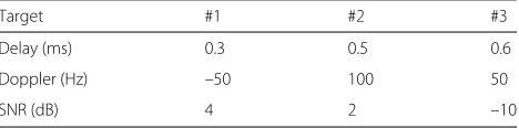
Table 2Target echo parameters in scenario #1
Target #1 #2 #3
Delay (ms) 0.3 0.5 0.6
Doppler (Hz) –50 100 50
a
b
c
Fig. 6The ambiguity function output in dB before cancellation in scenario #1.a2-D output.bSection at delay 0.cSection at Doppler 0
algorithms. Initially, the CA and TA are written as follows:
CA=10 log
input clutter amplitude peak output clutter amplitude peak
, (24)
a
b
Fig. 7The ambiguity function output in dB after direct signal and all clutter cancellation(k=50,p=1 andM=150)by the ECA algorithm in scenario #1.a2-D output.bSection atl=0
TA=10 log
input target amplitude peak output target amplitude peak
, (25)
where, the phrases “input clutter/target amplitude peak” and “output clutter/target amplitude peak” indicate the amplitude of clutter/target before and after the clut-ter and direct signal cancellation, respectively. For eval-uating the SCB algorithm in comparison with the ECA, SCA and ECA-B algorithms using the CA and
Table 3Selected parameters for simulation of the SCB algorithm
Observation time Tint 1 s
Sampling time Ts 0.005 ms
a
b
c
e
d
Fig. 8The ambiguity function output in dB after direct signal and all clutter cancellation by the SCB algorithm with Doppler bin(−1, 0, 1)in scenario #1a. 2-D output.bSection at Doppler –50 Hz.cSection at Doppler 100 Hz.dSection at delay 0.3 ms.eSection at delay 0.5 ms
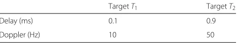
TA tests, we consider scenario #2 containing one target and one clutter (spot clutter1 or exponential spectrum clutter2) with characteristics tabulated in Table 4.
According to scenario #2, we obtain the values of CA and TA of the algorithms. For clutter and direct signal cancellation, p is considered as −1, 0 and 1. Since the CA and TA of SCB algorithm depend on the number of batches (b), we consider these quantities for various values of b. In Fig. 10, a simulated CA curve of the SCB algorithm is depicted versus the number of batches in comparison with that of the ECA, ECA-B and SCA algorithms. It is observed that the CA of SCB and ECA-B is similar, and when the clutter has an exponential spec-trum, the CA is reduced by 6 dB (in both SCB and ECA-B
methods). It is seen that the CA of SCB with ten batches
(b = 10) is close to that of ECA and SCA. By increas-ing b from 10 to 30, the CA of SCB increases. For b more than 30, further attenuation for clutter is no longer available.
a
b
c
Fig. 9The ambiguity function output in dB after direct signal, all clutters, and strong target cancellation by SCB algorithm in scenario #1.a2-D output.bSection at Doppler 50 Hz.cSection at delay 0.6 ms
that the TA of SCB and ECA-B is similar, and when the clutter has an exponential spectrum, the TA is not changed.
Table 4Clutter and target parameters in scenario #2 for calculation of CA and TA in SCB, ECA and SCA algorithms
Delay (ms) Doppler (Hz) SNR (dB)
Clutter1 0.25 0 25
Clutter2 0.25 Exponential Spectrum between−1 and 1 Hz
25
Target 0.6 100 5
4.2 Evaluation using CFAR target detection
In this section, in order to evaluate the proposed algo-rithm based on the target detection criteria, we use a CA-CFAR detector after clutter and direct signal cancellation using the mentioned algorithms. We use receiver oper-ating characteristic (ROC) curves for detection perfor-mance comparison. In this manner, first, clutter and direct signal are removed by the SCB (or ECA and ECA-B) algo-rithm, and then targets are detected based on the output of ambiguity function and CA-CFAR detector. The detec-tors based on the ECA, ECA-B and SCB algorithms are called ECA-CA, ECA-B-CA and SCB-CA, respectively.
For comparing the ECA-CA, ECA-B-CA and SCB-CA algorithms, we consider scenario #3 where targets have been placed according to Table 5 in Delay-Doppler page and there are nine clutters with fc = 0 (or
one clutter with exponential spectrum between −1 and 1 Hz), 5 dB < CNR < 30 dB and maxi-mum delay 0.3 ms, where CNR denotes clutter-to-noise ratio.
In Fig. 12, the curves of detection probabilityPdversus SNR of ECA-CA, ECA-B-CA and SCB-CA detectors are plotted for nominal probability of false alarmPfa=0.01.
It is observed that the ROC of SCB and ECA-B is similar, and when the clutter has an exponential spec-trum SNR is reduced to 4 dB in both methods. It is
10 20 30 40 50 60 70 80 90 100
42 44 46 48 50 52 54 56 58 60 62 64
Number of batches
CA(dB)
SCB ECA SCA ECA−B
SCB(Exp. spectrum) ECA−B(Exp. spectrum)
10 20 30 40 50 60 70 80 90 100
Fig. 11The TA curve of SCB versus the number of batches in comparison with that of ECA, ECA-B and SCA in scenario #2
seen that by decreasing the number of batch in the SCB algorithm, the performance of the SCB-CA improves so that the ROC of SCB-CA with b = 10 is close to the ROC of ECA for both targets T1 and T2. This means the SCB-CA detector performs similar to the ECA-CA detector if the number of batch is low. Consider that the SCB-CA has less computational complexity than that of ECA-CA. The ECA-CA and SCB-CA detec-tors degrade if Doppler frequency of target tends to be 0 Hz.
5 Conclusions
In this paper, the SCB algorithm is proposed for cancel-lation of static and non-static clutters as well as elimina-tion of direct signal component in passive bistatic radars based on projections of the received signals onto a sub-space orthogonal to the signal subsub-space of the clutter and the subspace of the previously detected targets. The SCB algorithm is first used for clutter and direct signal cancellation and detection of strong targets. To enhance the detection performance, the observation algorithm is then investigated and applied for detection of targets with weak signals. The simulation results revealed that the SCB algorithm performers well in the detection of targets com-pared with the state-of-the-art methods. The TA, CA and CFAR detection tests were used for comparing the SCB with the ECA, ECA-B and SCA algorithms. These tests
Table 5Clutter and target parameters in scenario #2 for calculation of CA and TA in SCB, ECA, ECA-B and SCA algorithms
TargetT1 TargetT2
SCB−CA (b=10) target T1
SCB−CA (b=20) target T1
ECA−CA target T2
SCB−CA (b=10) target T2
SCB−CA (b=20) target T2
ECA−B−CA (b=20) target T
1
ECA−B−CA (b=20) target T2
SCB−CA (b=20&Exp.sp.) T1
SCB−CA (b=20&Exp.sp.) T2
ECA−B−CA(b=20&Exp.sp.)T2
ECA−B−CA(b=20&Exp.sp.)T1
Fig. 12The curves of detection probability versus SNR of ECA-CA, ECA-B-CA and SCB-CA detectors for nominal probability of false alarm Pfa=0.01 in scenario #3
showed that targets may hide in the ambiguity function when the number of batches increases. The SCB algo-rithm has lesser computational complexity than the ECA and ECA-B algorithms. Moreover, the proposed method requires lesser memory than these algorithms and the SCA method.
Competing interests
The authors declare that they have no competing interests.
Author details
1Department of Electrical and Computer Engineering, Yazd University,
89195-741 Yazd, Iran.2Department of Electrical and Computer Engineering, Isfahan University of Technology, Isfahan 84156-83111, Iran.3Department of Electrical and Computer Engineering, Queen’s University, 99 Union St., Kingston ON K7L 3N6, Canada.
Received: 24 July 2016 Accepted: 25 November 2016
References
1. HD Griffiths, NR Long, Television based bistatic radar. IEE Proc. Part F Commun. Radar Signal Process.133, 649–657 (1986)
2. F Ansari, MR Taban, Clutter and direct signal cancellation in analog TV-based passive radar. Radar.1, 1–14 (2014)
3. A Lauri, F Colone, R Cardinali, P Lombardo, inProceedings of IEEE International Conference on Aerospace. Analysis and emulation of FM radio signals for passive radar (IEEE, Big Sky, MT, 2007)
4. M Cherniakov, inProceedings of IET International Conference on Radar. Space-surface bistatic synthetic aperture radar prospective and problems (IET, Edinburgh, 2002)
5. HA Harms, LM Davis, J Palmer,Understanding the signal structure in DVB-T signals for passive radar detection. (IEEE, Washington, 2010)
6. D Poullin, Passive detection using broadcasters (DAB, DVB) with CODFM modulation. IEE Proc. Radar Sonar Navigation.152, 143–152 (2005) 7. D Tan, H Sun, Y Lui, M Lesturgie, H Chan, Passive radar using global
system for mobile communication signal: theory, implementation and measurements. IEE Proc. Radar Sonar Navigation.152, 116–123 (2005) 8. PE Howland, D Maksimiuk, G Reitsma, FM radio basedbistatic radar.
IEE Proc.Radar Sonar Navigation.152, 107–115 (2005)
10. A Zaimbashi, M Derakhtian, A Sheikhi, GLRT-based CFAR detection in passive bistatic radar. IEEE Trans. Aerospace Electron. Syst.49, 134–159 (2013)
11. A Zaimbashi, M Derakhtian, A Sheikhi, Invariant target detection in multiband FM-based passive Bistatic radar. IEEE Trans. Aerospace Electron. Syst.50, 720–736 (2014)
12. J Palmer, SJ Searle, inProceedings of IEEE International Conference on Radar. Evaluation of adaptive filter algorithms for clutter cancellation in passive bistatic radar (IEEE, Atlanta, 2012)
13. F Wang, inProceedings of IET International Conference on Radar. Direct signal recovery and masking effect removal exploiting sparsity for passive bistatic radar (IET, Hangzhou, 2015)
14. F Colone, R Cardinali, P Lombardo, inProceedings of IEEE International Conference on Radar. Cancellation of clutter and multipath in passive radar using a sequential approach (IEEE, Verona, 2006)
15. F Colone, DW O’Hahan, P Lombardo, CJ Baker, A multistage processing algorithm for disturbance removal and target detection in passive bistatic radar. IEEE Trans. Aerospace Electron. Syst.45, 698–722 (2009)
16. A Ansari, MR Taban, inProceedings of Iranian Conference on Electrical and Electronic Engineering (ICEE2013). Implementation of sequential algorithm in batch processing for clutter and direct signal cancellation in passive bistatic radars (IEEE, Mashhad, 2013)
17. F Colone, C Palmarini, T Martelli, E Tilli, Sliding extensive cancellation algorithm (ECA-S) for disturbance removal in passive radar. IEEE Trans. Aerospace Electron. Syst.52, 1326–1309 (2016)
18. K Kulpa, inProceedings of Microwaves, Radar and Remote Sensing. The clean type algorithms for radar signal processing (IEEE, Kiev Ukraine, 2008) 19. RD Fry, DA Gray, inProceedings of International Conference on Radar. Clean
deconvolution for sidelobe suppression in random noise radar (IEEE, Adelaide, 2008)
20. C Jinli, Z Xiuzai, L Jiaqiang, G Hong, inProceedings of IEEE International Conference on Information Science and Technology (ICIST). Ground clutter suppression using noise radar with dual-frequency transmitter (IEEE, Hubei, 2012)
21. K Kulpa, Z Czekala, Masking effect and its removal in PCL radar. I EE Proc. Radar Sonar Navigation.152, 174–178 (2005)
Submit your manuscript to a
journal and benefi t from:
7Convenient online submission
7Rigorous peer review
7Immediate publication on acceptance
7Open access: articles freely available online
7High visibility within the fi eld
7Retaining the copyright to your article