R E S E A R C H
Open Access
Autonomous radar pulse modulation
classification using modulation
components analysis
Pei Wang
*, Zhaoyang Qiu, Jun Zhu and Bin Tang
Abstract
An autonomous method for recognizing radar pulse modulations based on modulation components analysis is introduced in this paper. Unlike the conventional automatic modulation classification methods which extract modulation features based on a list of known patterns, this proposed method classifies modulations by the existence of basic modulation components including continuous frequency modulations, discrete frequency codes and discrete phase codes in an autonomous way. A feasible way to realize this method is using the features of abrupt changes in the instantaneous frequency rate curve which derived by the short-term general representation of phase derivative. This method is suitable not only for the basic radar modulations but also for complicated and hybrid modulations. The theoretical result and two experiments demonstrate the effectiveness of the proposed method.
Keywords:Autonomous modulation classification, Modulation components analysis, Sliding window, Abrupt changes, Instantaneous frequency rate
1 Introduction
Pulse modulation classification plays an essential role in modern intercept receivers for electronic warfare (EW) applications such as threat recognition and analysis, con-struction of effective jamming responses and radar emit-ter identification [1]. In the EW context, modulations on radar pulses are divided into two classes, the intentional modulation on pulse (IMOP) and the unintentional modulation on pulse (UMOP). The feature of UMOP is usually applied for the purpose of specific emitter identifi-cation while the feature of IMOP is mainly used to collect intelligence of a hostile radar system [2]. Pulse modulation classification is a technique aiming at recognizing the intentional intra-pulse modulations of radar signals and is becoming more and more difficult because of the ever-increasing number of emitters and low probability of intercept (LPI) radar waveforms that have appeared in modern electromagnetic environment [3]. The newly emerging radar systems, such as the cognitive radar [4], the waveform-agile radar [5], and the multiple-input multiple-output (MIMO) radar [6, 7], are changing their
operation modes and bringing waveforms with various kinds of complicated IMOPs. Apart from that, some wave-forms with hybrid IMOPs, such as the discrete phase codes on linear frequency modulation (LFM) [8, 9], mul-tiple frequency-shift keying (FSK) waveform outperformed by a chirp modulation [10], and the combination of FSK and phase-shift keying (PSK) modulations [11], have also been reported. These complicated and hybrid IMOPs are posing a particular threat to modern EW intercept receivers.
However, nearly all of the existing pulse modulation classification algorithms are realized based on some known emitter databases and are suitable only for a certain group of IMOPs [12]. For example, an atomic decomposition method employing chirplet dictionary was proposed in [13], and it can realize the automatic detection and classification of radar pulses with LFM, PSK, and FSK modulations. An supervised classification system achieving overall correct classification rate of 98 % at signal-to-noise ratio (SNR) of 6 dB based on multilayer perception networks was proposed in [14] and eight classes of radar signals are classified. Algo-rithms based on some time-frequency distributions such * Correspondence:[email protected]
School of Electronic Engineering, University of Electronic Science and Technology of China, Chengdu, China
as the ambiguity function (AF) [15], Zhao Altas and Marks (ZAM) representations [16], the Rihacek distribu-tion and the Hough transform [17], were also applied to extract modulation features for five kinds of radar pulses. These existing algorithms work effectively when the radar IMOPs are in the list of their databases, but fail when they are faced with some complicated or un-known modulated pulses.
In this paper, we try to classify radar pulse modulations using an autonomous method. A two-stage classification procedure which contains a“modulation family classifica-tion” and an “accurate classification” is proposed. The former part works autonomously based on a modulation components analysis (MCA) method and can extract par-tial information even when the IMOP of the radar pulse is not in the knowledge database. The latter part is a supple-mentary part to classify an IMOP in detail and is exten-sible. The paper is organized as follows. Section 2 gives a universal category of IMOPs and describes signal models using the instantaneous frequency rate (IFR) curves. Section 3 describes the whole classification procedure of the proposed method. Two experiments to demon-strate the effectiveness of the proposed method are designed in Section 4, and Section 5 gives the main conclusions.
2 Signal model and abrupt changes analysis in IFR curve
2.1 Categories of possible radar pulse modulations In order to analyze the various kinds of IMOPs conveni-ently, we categorize them based on three kinds of basic IMOP components including the continuous frequency modulation (CFM), the discrete frequency coded (DFC) modulation and the discrete phase coded (DPC) modu-lation. Possible IMOPs in CFM class include constant frequency (CF), LFM and various nonlinear frequency modulations (NLFM). The DFC class contains binary frequency codes (BFC), the Costas codes and so on. The DPC class includes IMOPs such as binary phase codes (BPC), quadriphase codes (QPC) and polyphase codes (PPC).
Various modulations can be realized by a single IMOP or combinations of different IMOPs. According to the phase properties between different IMOPs, three modu-lation families are extended as the CFM family, the DFC family and the DPC family as shown in Fig. 1. But be-yond that, a fourth family which contains intra-pulse modulation agile waveform, noise-like waveform and so on may also appear. For the convenience of analysis, here, we consider only the former three families. It is easy to see that not only the common radar pulse modu-lations that have been used so far, but also the existing and possible complicated or hybrid modulations are under this context.
2.2 Signal model
For the intercept receivers, the received radar pulse could be modeled as follows
r tð Þ ¼s tð Þ þw tð Þ
¼Aexpðjϕð Þt Þ þw tð Þ; 0≤t≤T ð1Þ
where T is the pulse duration time, A is the complex amplitude of the signal, ϕ(t) is phase of the intercepted radar pulse, and w(t) is the complex additive white Gaussian noise (AWGN) with variance σ2. The corre-sponding discrete model is
r nð Þ ¼Aexpðjϕð Þn Þ þw nð Þ; n¼0;…;N ð2Þ where the sampling frequency isfs.
To identify an unknown, or a complicated modulated radar pulse, we should find out which basic modulation exists and that is why we call the method as“MCA”. For a signal in the CFM family, the phase function can be considered as a polynomial phase signal according to the Weierstrass theorem.
the highest order of the polynomial coefficients.
For a signal in the DFC family, the basic modulation is frequency coding.
whereMis the number of sub-pulses,fkis the carrier
fre-quency of the kth sub-pulse,Tpis the width of sub-pulse,
andg(t) is a rectangular function andg(t) = 1 when 0≤t<
Tp. Considering complicated modulations such as hybrid
modulations of CFM and basic DFC components, the phase function of a signal in DFC family can be expressed as
ϕDFCð Þ ¼t ϕCFMð Þ þt ϕBasicDFCð Þt ð5Þ
For a signal in the DPC family, the basic modulation is phase coding.
ϕBasicDPCð Þ ¼t
X
k¼0 L−1
θkg t−kTð cÞ; 0≤t≤T ð6Þ
where L is the number of phase codes; θk is kth phase
and Tc is the width of phase code. Considering
com-plicated modulations such as hybrid modulations of basic DPC modulations with CFM or DFC modulations, the phase function of a signal in DFC family can be expressed as
ϕDPCð Þ ¼t ϕCFMð Þ þt ϕBasicDFCð Þ þt ϕBasicDPCð Þt ð7Þ
The MCA method distinguishes basic modulation components based on the abrupt changes in their phase derivatives. Here the IFR curve is used as example.
2.3 IFR propertis for basic modulation components The direct derivation of IFR is the second derivative of signal phase which can be expressed as:
IFR tð Þ≜ 1
2π
d2ϕð Þt
dt2 ð8Þ
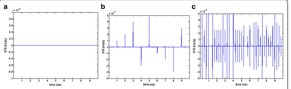
Different modulation families show different proper-ties in their IFR curves. For convenience, three basic modulations which belong to different modulation fam-ilies are considered here in discrete case.
For the basic modulation in the CFM family, the IFR is shown as
IFRCFMð Þ ¼n
1
πa2þζð Þn ð9Þ
where ζ(n) is a polynomial phase function. Thus, there are no abrupt changes in the IFR curve. The IFR curve of an LFM pulse is shown in Fig.2a.
The IFR of a basic DFC modulation is
IFR nð Þ ¼fsX
k¼1 M
fk−fk−1
δ n−kTp
ð10Þ
where δð Þ ¼n 1; n¼0
0;otherwise
. Thus, an abrupt change
appears if the adjacent sub-pulses have different frequencies and the amplitude of the abrupt change de-pends on the difference of the two adjacent frequencies. The IFR curve of a Costas coded pulse is shown in Fig.2b.
The IFR of a basic DPC modulation is
IFR nð Þ ¼ f
2 s
2π X
k¼1 M
ck−ck−1
ð Þðδðn−1−kTcÞ−δðn−kTcÞÞ
ð11Þ
There will be two abrupt changes which have a same absolute value and opposite signs in the IFR curves and the amplitude of the abrupt changes depend on the adjacent phases. The IFR curve of a QPC pulse is shown in Fig. 2c.
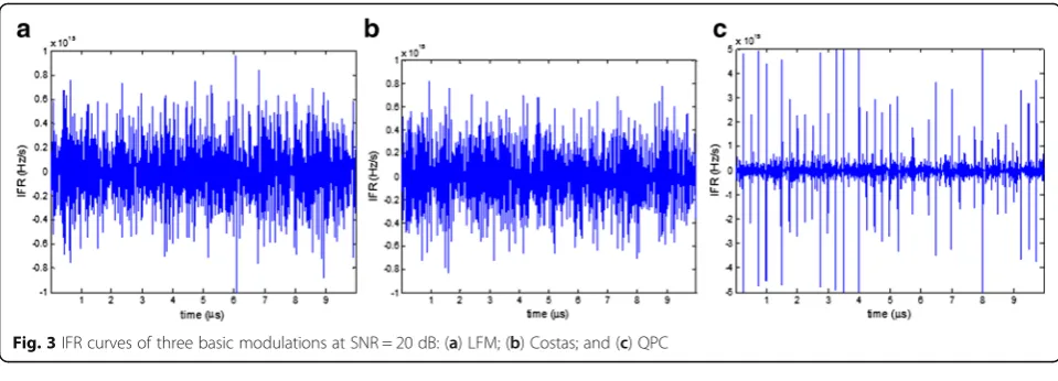
A traditional way to approximately realize the phase derivatives is using phase unwrapping and phase differ-ence operations. But, it suffers a rapid degradation of performance even at a high SNR. Figure 3 shows the estimated IFR curves of the same three pulses using the phase-based way at SNR = 20 dB, and it seems impos-sible to extract the features of abrupt changes in the IFR curves especially for the DFC signal.
2.4 Robust IFR estimation and abrupt changes analysis As the MCA method analyzes the abrupt changes in the IFR curves, methods which are robust to noise and sensitive to abrupt changes need to be found. The IFR estimation was firstly used for chirp signal estimation [18] and the concept of any order phase representation was generalized through the term of general representa-tion of phase derivative (GRPD) [19]. In [20], the IFR
was derived using the short-term polynomial phase esti-mation in the EW context and the influence of window length on parameter estimation was analyzed. On the basis of previous studies, we will extract features from the abrupt changes in the IFR curves and then classify the modulation family autonomously in this paper.
The GRPD method is a kind of multi-linear method which is suitable for IFR estimation. It has been proved that the GRPD method using a sliding window has a good performance which approaches the Cramer-Rao bound (CRB) for the IFR estimations [20]. According to the GRPD theory, the ideal representation of an arbitrary instantaneous phase derivative (IPD) of a signal can be written in the form
IPDKðt;ΩÞ ¼A2δ Ω−ϕð ÞKð Þt
ð12Þ
where Ω is the axis which corresponds to the Kth derivative of the phase function ϕ(t). In order to obtain the distribution concentrated along Kth phase derivative, a generalized complex moment (GCM) is defined as
For example, when N= 1, it leads to the short-time Fourier transform (STFT), and when N= 2, it leads to a Wigner-Ville-like distribution.
WhenK= 2, it is a time-“frequency rate”representation.
GCM2N½ sðt;τÞ ¼Y
To calculate the IFR, here, we consider a simple case forN= 2. Therefore, the GCMs are
GCM22½s;tið Þ ¼τ s tþ
estimated using a short-time window by the relations as follows.
Supposing that the length of sliding window in calculating the IFR value at a certain time instant isNw, it can be approved that [20]
CRB IFR tf ð Þi g ¼
1 π2
90f4s
N5wSNR: ð18Þ
Therefore, for a given SNR and a given mean square error (MSE) of estimators, the length of the sliding win-dow should satisfy the following relation.
Nw≥
Figure 4 shows the estimated IFR curves of the same three pulses in Figs. 2 and 3 at SNR = 3 dB.
It shows that the short-time GRPD method is robust to noise and sensitive to abrupt changes. Therefore, the IFR curves are feasible to realize the autonomous MCA method.
3 Autonomous modualtion classification flow based on the MCA method
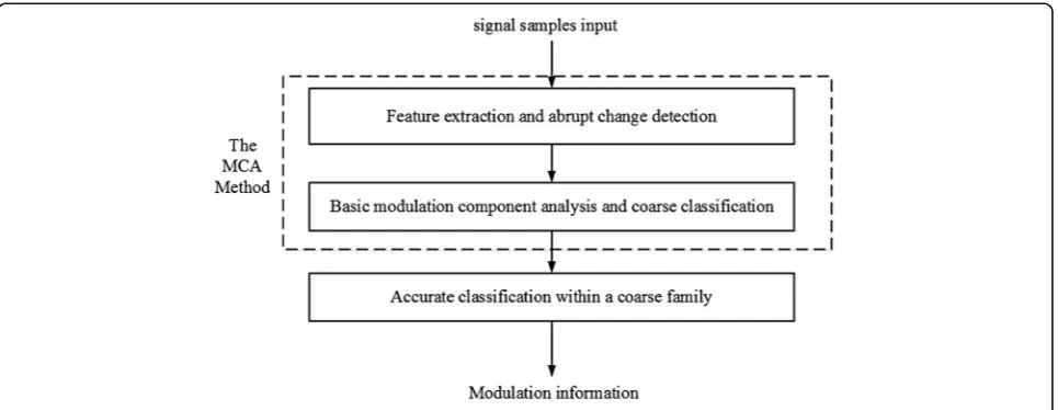
The autonomous classification methods focus on the essential differences among the three basic IMOPs. Here, we employ the abrupt changes caused by the DFC and the DPC modulations in the IFR curves. The signal processing flow for radar pulse modulation classification is shown in Fig. 5.
The modulation information is given after three steps. The samples of pulse will be processed to extract some modulation features. Then the MCA method is applied to classify the pulse into a modulation family and this can be also called a“coarse classification”. At last, an ac-curate classification will be done within the modulation family and some possible modulation parameters will be estimated at the same time using existing algorithms.
3.1 Modulation families classification based on MCA method
From the analyses above we know that the estimated IFR curve for an IMOP in the CFM family has no abrupt
changes. Thus a basic CFM component can be distin-guished from the DFC and the DPC families. The esti-mated IFR curve using a short-time window of a pure DFC components has abrupt changes regularly. Once a change appears, its values will keep positive or negative for a short period. By contrast, the abrupt changes in the estimated IFR curve for a basic DPC component appear mixed and disorderly. According to the differences of abrupt changes, we can recognize the IMOP family of a pulse autonomously. Figure 6 shows the modulation fam-ily classification flow based on the MCA method.
The flow chart contains several important modules: SNR estimation and sliding window setting module, IFR estimation module, and abrupt changes analysis module.
3.1.1 SNR estimation and sliding window setting
SNR is an important parameter in signal processing. When it comes to a non-cooperative situation, a simple and effective method to estimate the SNR is the 2nd and 4th order moments (M2M4) algorithm [21, 22]. This Fig. 4Estimated IFR curves of three basic modulations at SNR = 3 dB: (a) LFM; (b) Costas; and (c) QPC
MSEs of the M2M4 algorithm approaches its theoretical variance for SNR >−5 dB and SNR < 15 dB [22]. In this paper, we assume that the classification problem is considered when the M2M4 algorithm works well. For the discrete receiving signal in AWGN, it is easy
to calculate the 2nd order moment M2 and 4th order
moment M4.
where E[•] is the mathematical expectation of the random receiving variables and the mark ‘≅’ means “approximately equals to”. Thus the estimated SNR is expressed as
Given a requested MSEσ2IFR of the IFR estimation, the length of the window can be obtained by (19).
b gives the minimum integral value that satisfies the equa-tion. From the above equation, we can calculate that if
the estimatedSNR^ has a maximum error of 0.5 dB, then the length of the sliding window has a maximum error of less than 3 %. Therefore, the length of the sliding win-dow can be estimated accurately when the M2M4 algorithm works well.
3.1.2 IFR estimation using a sliding window
To realize the IFR estimation by (17), some parameters should be considered according to the signal processing capability and they are adjustable for the algorithm de-signer. These parameters are:
The maximum valueIFRmaxof the possible IFRs, The minimum valueIFRminof the possible IFRs, The IFR increment or the step lengthΔIFR, and The length sliding windowNwin, an odd number
that satisfiesNwin≥Nbw.
For a given time instant nc, the IFR can be calculated using the window with lengthNwb .
IFR nð Þ ¼c
2 is a transform matrix to
calcu-late the IFR and NIFR is the number of possible IFR
elements.
by the abrupt changes range from IFRmin to IFRmax, the proposed MCA method will perform well.
3.1.3 Abrupt changes analysis and the thresholds in IMOP family recognition
We set the thresholds in the MCA method through Monte Carlo simulations for a broad span of SNR and modulations. The threshold Th1 follows two strategies and is a trade-off between two sub-thresholds,Th01and Th02. Th01 is an SNR-dependent threshold and Th02 is an SNR-independent threshold related to the signal pro-cessing capability. For a signal in the CFM family, there are no abrupt changes in the IFR curve in theory. How-ever, some outliers that seem like abrupt changes may appear when the signal is disturbed by noise. Assuming that the ratio of abrupt changes in the IFR curve is α and Th1 is used to distinguish it from the other two IMOP families. According to the properties of a CFM Fig. 6Modulation family classification flow chart based on the
modulation, the threshold should be a slowly decreasing function of SNR values and always positive. By the Monte Carlo simulations for a broad span of SNR values, a pos-sible threshold can be defined as
T h01¼ρexpð−SN RÞ=SNR ð27Þ
whereρ∈(0, 1) is a small coefficient. On the other hand, the SNR-independent threshold Th02 is related to the maximum ratio η1 of abrupt changes in the IFR curve for a CFM modulation at low SNR.
T h02¼η1 ð28Þ
Thus, the thresholdTh1 should be
T h1¼ minðT h01;T h02Þ ð29Þ
where min(•) is the minimum value function. Ifα>Th1, it means that the abrupt changes caused by modulations are detected.
The thresholds Th2 and Th3 are used to determine
whether an IMOP belongs to DFC family or DPC family. The ratio of the regular changes in all abrupt changesβ
and the number of change segments Nseg are defined
here. From the analyses above, we conclude that β is
close to 1 when the IMOP belongs to the DFC family at high SNR while it approximates 0 when the IMOP is a DPC modulation.Th2 is a threshold to evaluate the pro-portion of regular changes in all abrupt changes.
T h2¼η2 ð30Þ
According to the majority rule, there isη2∈(0.5, 1) for an IMOP in the DFC family. In order to increase the re-liability of recognition, the threshold Th3 is set to
com-pare with the number of change segments Nseg. While
the window slides along the received signal samples, there is at most one change segment caused by the adja-cent sub-pulses for signal in the DFC family. It means that the maximum number of change segments for DFC modulation will not be bigger than the number of sub-pluses. However, as the signal processing is non-cooperative, the number of sub-pulses is difficult to ob-tain. Here, we assume that the number of points of the sliding window is less than that of a sub-pulse; therefore, we have
T h3¼N=Nwin: ð31Þ
Thus, a modulation type belongs to the DFC family will be recognized ifβ>Th2 andNseg<Th3.
The thresholds Th01 and Th3 change their values
autonomously for different intercepted signals with dif-ferent SNRs whileTh02 and Th2 are optional empirical thresholds which can improve classification performance according to noise level. So far, the IMOP families are recognized using the MCA method.
3.2 Accurate modulation classification within modulation families
The MCA method based on the abrupt changes can only classify an IMOP into a modulation family. If more infor-mation of an intercepted pulse is wanted, it is necessary to carry out an accurate modulation classification within a certain modulation family. Thus, it becomes a new classi-fication problem. Four basic IMOPs including the CF, LFM, BPC, and BFC modulations are considered here as examples. The modulation features are extracted from the instantaneous phase and instantaneous frequency law (IFL) curve which is calculated according to (14) and (17).
d
For the BFC modulated signal in the DFC family, we can recognize it by counting the number of frequencies in the IFL curve. For the BPC modulated signal in the BPC family, we can recognize it by determining whether the squared signal shows properties of a CF modulation. For an IMOP in the CFM family, we use the piecewise linear fitting method to the IFL curve. The mean square errors are derived between the instantaneous frequency and its least squares linear fitting. The corresponding classification flow is carried out as follows.
(1)Estimate the IFL curves and do linear fitting to get the corresponding initial frequencyfLF0and chirp ratekLF0.
(2)Divide the IFL into two equal pieces and do linear fitting to each piece to getfLF1,kLF1andfLF2,kLF2, and here, we suppose thatkLF1≥kLF2.kmaxis the
maximum of the two absolute values |kLF1| and |kLF2|. (3)Calculate the ratios,rf1=fLF1/fLF0,rf2=fLF2/fLF0,
rk=kLF1/kLF2
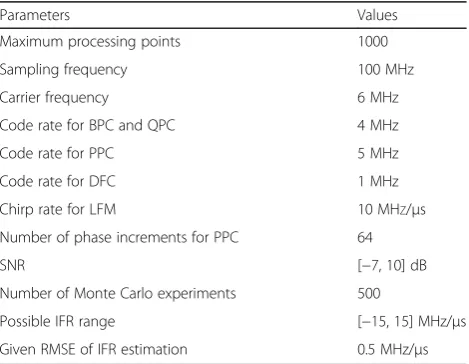
Table 1Parameters for radar pulse generation and signal processing
Parameters Values
Maximum processing points 1000
Sampling frequency 100 MHz
Carrier frequency 6 MHz
Code rate for BPC and QPC 4 MHz
Code rate for PPC 5 MHz
Code rate for DFC 1 MHz
Chirp rate for LFM 10 MHZ/μs
Number of phase increments for PPC 64
SNR [−7, 10] dB
Number of Monte Carlo experiments 500
Possible IFR range [−15, 15] MHz/μs
(4)Ifrth1≤rf1≤rth2,rth1≤rf2≤rth2, andkmax≤kmaxTh, the IMOP is determined as a CF modulation. Otherwise, ifrth1≤rk≤rth2, the IMOP is determined as an LFM.
The thresholds rth1, rth2 and kmaxTh are determined
according to the maximum errors which can be designed at the initial stage of the signal processing procedure. The accurate modulation classification is realized based on the known modulation families.
4 Results and discussion
Two experiments are designed to demonstrate the ef-fectiveness of the proposed method. The first one is used to check the performance of the MCA method and radar pulses are classified into different IMOP families. The second one is designed to classify four commonly used IMOPs by accurate classification within their IMOP families and the results are compared with the AF-based
method [15]. In these two experiments, we evaluate the performances by the probability of successful modulation family recognition (PSMFR) and the probability of suc-cessful modulation recognition (PSMR) which are both calculated using the Monte Carlo experiments. The simu-lation parameters are shown in Table 1.
In the MCA method, the coefficientρ inTh01is set as
0.25 and the maximum ratio of abrupt changes η1 for
the CFM components in Th02is set as 0.2, and the pro-portion of regular changes in all abrupt changes for the DFC componentsη2is set as 0.7. In the accurate modu-lation classification part, thresholdrth1is set as 0.8 while rth2is set as 1.2. The maximum valuekmaxThfrom a CF
modulated signal is set as 1011 Hz/s which is related to minimum chirp rate for an LFM signal. These thresholds are verified by a broad band of experiments.
4.1 Autonomous classification for modulation families The first experiment gives the performance of the pro-posed MCA method. The simulation adopts modula-tions in Table 2. The three kinds of hybrid modulamodula-tions are the LFM-BFC modulation [10] in the DFC family and the LFM-BPC [8, 9] and the BPC-BFC [11] modula-tions in the DPC family.
Figure 7 gives the probabilities of successful modula-tion family recognimodula-tion (PSMFRs) for the simulated
Table 2The IMOPs for the MCA method in the simulation
Modulation family IMOPs
CFM CF, LFM, VFM, SFM
DFC BFC, Costas coding, LFM-BFC,
DPC BPC, QPC, Frank, P1, P2, P3, P4, LFM-BPC, BPC-BFC
IMOPs. Figure 7a shows that the PSMFRs for the signals in the CFM family reach 98 % when the SNR is
above −3 dB. These signals have similar PSMFRs and
the reason is that they are classified by the same threshold Th1. Figure 7b shows the PSMFRs of BFC and Costas coded signals in the DFC family, and they can be classified well when the SNR is above 3 dB. In Fig. 7c, several IMOPs in the DPC family are classi-fied and can be classiclassi-fied well when the SNR is above 4 dB. Figure 7d gives the PSMFRs of three hybrid modulations, and the proposed method achieves a successful probability of 95 % for the three kinds of signals when the SNR is above 2 dB. This experiment shows that the MCA method can give partial infor-mation about the modulation family for various kinds of IMOPs.
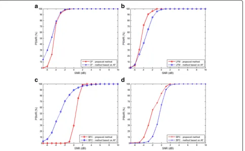
4.2 Accurate classifications for four basic radar pulse modulations
This experiment is designed to verify how the proposed method performs compared with the method based on the AF properties [15]. As the comparison method can only deal with a limited number of IMOPs, we do our experiment here for the four commonly used basic IMOPs, the CF, LFM, BPC, and BFC modulations. For a better comparison, we choose the pulse width as 5 μs
which has been used in [15]. The PSMRs are calculated using 1000 Monte Carlo trials for each SNR value. The PSMRs for the above four kinds of IMOPs are shown in Fig. 8.
For the CF signals, Fig. 8a shows that the proposed method and the comparison method have nearly the same PSMRs which are greater than 96 % when the SNR
is above −2 dB. The PSMRs for the LFM signals
ap-proaches 100 % for both of the two signals when the SNR is above 0 dB in Fig. 8b. However, the proposed method performs better than the comparison method when the SNR decreases. In Fig. 8c, we see that the PSMRs are greater than 97 % when the SNR is above 2 dB. The comparison method has slow increasing
PSMRs when the SNR values ranges from −6 to 2 dB
while the proposed method has steep rising PSMRs when the SNR is close to 1 dB. For the BPC signals, the PSMRs for both methods are greater than 98 % as Fig. 8d shows when the SNR is above 2 dB and the proposed method has a slightly better performance than the comparison method when the SNR is smaller than 2 dB. Figure 8 shows that the proposed method and the com-parison method differ slightly only when the SNR is below 2 dB.
From the two experiments above, we know that if an IMOP has features matched with a known database, it
can be recognized with a similar overall performance to the method based on the AF properties whose PSMR is more than 96 % when the SNR is above 2 dB. However, if an IMOP does not belong to a known database, the proposed method can still work and obtain partial infor-mation by classifying it into a modulation family while the conventional methods fail to work. In general, the proposed method gives a different classification structure for classification methods of radar pulse modulations. What is more, the accurate modulation classification part can be extended easily within a certain modulation family.
5 Conclusions
A two-stage pulse modulation classification method which contains a “modulation family classification” and an “accurate classification” is presented. The former stage is autonomously realized based on the proposed MCA classification method and different IMOPs are classified into three modulation families based on the abrupt change features extracted from the IFR curves. A final decision is done by the latter stage which provides supplementary information for accurate classifications. This method can deal with a broad range of IMOPs and gives partial or complete modulation information while the existing methods give complete information for only a limited number of IMOPs. The theoretical analysis is validated by two designed experiments. The proposed method gives a different classification structure for radar pulse modulations and can be extended easily. Future work will focus on the study of different realization methods for the MCA structure and the extension of the accurate modulation recognition part to some com-plicated or hybrid modulations.
Abbreviations
AF:Ambiguity function; AMC: Automatic modulation classification; AMFRR: Autonomous modulation family recognition rate; AWGN: Additive white Gaussian noise; BFC: Binary frequency codes; BPC: Binary phase codes; CFM: Continuous frequency modulation; CRB: Cramer-Rao bound; DFC: Discrete frequency coded; DPC: Discrete phase coded; EW: Electronic warfare; FSK: Frequency shift keying; GCM: Generalized complex moment; GRPD: General representation of phase derivative; IFL: Instantaneous frequency law; IFR: Instantaneous frequency rate; IMOP: Intentional modulation on pulse; LFM: Linear frequency modulation; LPI: Low probability of intercept; MCA: Modulation components analysis; MIMO: Multiple-input multiple-output; M2M4: 2nd and 4th order moments; NLFM: Nonlinear frequency modulations; PSK: Phase-shift keying; PPC: Polyphase codes; PSMFR: Probability of successful modulation family recognition; PSMR: Probability of successful modulation recognition; QPC: Quadriphase codes; SFM: Sine frequency modulation; SNR: Signal-to-noise ratio; UMOP: Unintentional modulation on pulse; VFM: V-shape frequency modulation
Acknowledgements
The authors thank the National Natural Science Foundation of China for their support for the research work. The authors also thank the reviewers for their suggestions and corrections to the original manuscript.
Funding
The work is supported by the National Natural Science Foundation of China, Grant No. 61571088 and No. 61172116.
Authors’contributions
The work presented here was carried out in collaboration between all authors. PW proposed the idea and structure of the autonomous classification and wrote the whole paper. ZQ and JZ found out the related literatures and co-designed the experiments. Professor BT gave important suggestions for the structure and experiment results of the paper. All authors have contributed to, seen, and approved the manuscript.
Competing interests
The authors declare that they have no competing interests.
Received: 29 April 2016 Accepted: 2 September 2016
References
1. RG Wiley, ELINT,The Interception and Analysis of Radar Signals(Artech House, Norwood, 2006), pp. 1–8
2. DL Adamy,EW 102: A Second Course in Electronic Warfare(Horizon House, Norwood, 2004), pp. 48–54
3. PE Pace,Detecting and Classifying Low Probability of Intercept Radar, 2nd edn. (Artech House, Norwood, 2009), pp. 1–37
4. S Haykin, Cognitive radar: a way of the future. IEEE Signal Process. Mag.23(1), 30–40 (2006)
5. SP Sira, Y Li, AP Suppappola, D Morrell, D Cochran, M Rangaswamy, Waveform-agile sensing for tracking. IEEE Signal Process. Mag. 26(1), 53–64 (2009)
6. W Huleihel, J Tabrikian, R Shavit, Optimal adaptive waveform design for cognitive MIMO radar. IEEE Trans. Signal Process. 61(20), 5075–5089 (2013)
7. S Wang, Q He, Z He, LFM-based waveform design for cognitive MIMO radar with constrained bandwidth. EURASIP J. Adv. Signal Process. 2014, 89 (2014)
8. DJ Lynch,Introduction to RF Stealth(SciTech Publishing, Releigh, 2004), pp. 336–343
9. M Ngwar, J Wight,Phase Coded Linear Frequency Modulated Waveform for Low Cost Marine Radar System, in Radar Conference(IEEE, Washington DC, 2010), pp. 1044–1049
10. M Kronauge, H Rohling, New chirp sequence radar waveform. IEEE Trans. Aero. Electron. Syst.50(4), 2870–2877 (2014)
11. JA Lemieux, FM Ingels,Analysis of FSK/PSK Modulated Radar Signals Using Costas Arrays and Complementary Welti Code.In Radar Conference(IEEE, Arlington VA, 1990), pp. 589–594
12. OA Dobre, A Abdi, YB Ness, W Su, Survey of automatic modulation classification techniques: classical approaches and new trends. IET Commun. 1(2), 137–156 (2007)
13. GL Risueño, J Grajal, OY Ojeda, Atomic decomposition-based radar complex signal interception. IEE Proc. Radar Son. Nav.150(4), 323–331 (2003)
14. H Lunden, V Koivunen, Automatic radar waveform recognition. IEEE J. Sel. Top. Signal Process.1(1), 124–136 (2007)
15. D Zeng, H Xiong, J Wang, B Tang, An approach to intra-pulse modulation recognition based on the ambiguity function. Circ. Syst. Signal Process. 29(6), 1103–1122 (2010)
16. D Zeng, X Zeng, G Lu, B Tang, Automatic modulation
classification of radar signals using the generalized time-frequency representation of Zhao, Altas and Marks. IET Radar Son. Nav. 5(4), 507–516 (2011)
17. D Zeng, X Zeng, H Cheng, B Tang, Automatic modulation classification of radar signals using the Rihaczek distribution and Hough transform. IET Radar Son. Nav.6(5), 322–331 (2012)
18. PO Shea, A fast algorithm for estimating the parameters of a quadratic FM signal. IEEE Trans. Signal Process.52(2), 385–393 (2004)
20. F Digne, C Cornu, A Baussard, A Khenchaf, D Jahan, inIET International Conference on Radar Systems (Radar 2012). Use of short-term polynomial phase estimation for new electronic warfare systems, (IEEE, Glasgow, UK, 2012), pp. 1–6
21. DR Pauluzzi, NC Beaulien, A comparison of SNR estimation techniques for the AWGN channel. IEEE Trans. Commun.48(10), 1681–1691 (2000) 22. LV Roberto, M Carlos, Sixth-order statistics-based non-data-aided SNR
estimation. IEEE Commun. Lett.11(4), 351–353 (2007)
Submit your manuscript to a
journal and benefi t from:
7 Convenient online submission
7Rigorous peer review
7 Immediate publication on acceptance
7Open access: articles freely available online
7 High visibility within the fi eld
7Retaining the copyright to your article