R E S E A R C H
Open Access
A generalized gamma correction
algorithm based on the SLIP model
Guang Deng
Abstract
Traditional contrast enhancement techniques were developed to enhance the dynamic range of images with narrow histograms. However, it is not unusual that an image with a broad histogram still suffers from low contrast in both the shadow and highlight areas. In this paper, we first develop a unified framework called the generalized gamma correction for the enhancement of these two types of images. The generalization is based on the interpretation of the gamma correction algorithm as a special case of the scalar multiplication of a generalized linear system (GLS). By using the scalar multiplication based on other GLS, we obtain the generalized gamma correction algorithm. We then develop an algorithm based on the generalized gamma correction algorithm which uses the recently developed symmetric logarithmic image processing (SLIP) model. We demonstrate that the proposed algorithm can be configured to enhance both types of images by adaptively choosing the mapping function and the multiplication factor. Experimental results and comparisons with classical contrast enhancement and state-of-the-art adaptive gamma correction algorithms demonstrate that the proposed algorithm is an effective and efficient tool for the enhancement of images with either narrow or broad histogram.
Keywords: Symmetric LIP model, Generalized linear system, Contrast enhancement
1 Introduction
1.1 Problem formulation
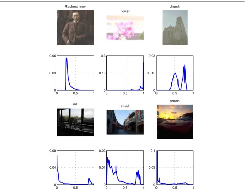
The contrast of an image is one of the most important factors influencing its subjective quality. An image, which is subjectively rated as low contrast, is usually associated with a limited dynamic range. In practice, pixels of an image can be broadly classified as either in the areas of shadow, mid-tone, or highlight. They correspond to pix-els in the lower end, middle part, and the higher end of the histogram, respectively. An image, which is classified as global low contrast, can have a narrow histogram in one of these areas. On the other hand, pixels of an image can be distributed mostly in the shadow and highlight areas which have limited dynamic ranges. Such an image is clas-sified as local low contrast. Figure 1 shows histograms of the six test images. The first three are typical cases of images with global low contrast, while the other three are typical cases of local low contrast.
Correspondence: [email protected]
Department of Engineering, La Trobe University, Bundoora, Victoria 3086, Australia
To enhance images of global low contrast, we can use classical dynamic range stretching algorithms such as his-togram equalization, gamma correction, and linear con-trast stretching [1]. However, since an image of local low contrast usually has a broad histogram, these algorithm may not produce the desired result.
In this work, we focus on the following problem: to develop a unified framework such that it can be used to enhance the two types of images.
1.2 A brief review of related works
Image enhancement is an active research area which has accumulated many papers on contrast enhancement. Contrast enhancement can be broadly classified as the fol-lowing: histogram-based methods such as many different ways of performing histogram equalization; linear con-trast stretching; nonlinear signal transformation such as gamma correction; and transform domain-based meth-ods such as performing enhancement in the wavelet or Fourier transform domain. Since this paper is on the gen-eralization of the gamma correction algorithm, we will only provide a brief review of some related works. Com-putational intensive image enhancement algorithms such
Rachmaninov
flower
church
0 0.5 1
0 0.03 0.06
0 0.5 1
0 0.15 0.3
0 0.5 1
0 0.015 0.03
iris street ferrari
0 0.5 1
0 0.04 0.08
0 0.5 1
0 0.01 0.02
0 0.5 1
0 0.05 0.1
Fig. 1First row: images of global low contrast.Second row: normalized histograms of images in the first row.Third row: images of local low contrast.
Fourth row: normalized histograms of images in the third row. Normalized histogram is the probability distribution function of pixels in an image
as the Retinex [2] and its variants including optimization through variational methods [3, 4] are not discussed.
In the following discussion, a pixel of an image is rep-resented by x where the spacial location of the pixel is omitted to simplify the notation. It is also assumed that the pixel gray scale has been normalized such that x ∈ (0, 1).
1.2.1 The logarithmic image processing model
In [5], the scalar multiplication operation of the logarith-mic image processing (LIP) model is used to enhance an image as follows:
y=γ1× x
=φ−1
LIP(γ1φLIP(x)) (1)
where φLIP(x) = −log(1 − x) and γ1 is an
image-dependent adaptive gain. It is determined by maximizing
the dynamic range of the processed image. The optimalγ is given by
γ1=
1
σ log μ+σ
μ−σ
(2)
whereμandσare the mean and standard deviation of the transformed image dataφLIP(x)= −log(1−x). However,
a drawback of this result is that it only works for images for which the conditionμ > σ is satisfied.
1.2.2 The parametric log-ratio model
In [6], the scalar multiplication operation of the paramet-ric log-ratio (PLR) model is used to enhance an image as follows:
y=γ2⊗x
=φ−1
where
φPLR(x)= −log
1−x
ηx (4)
The multiplication factorγ2and the model parameter
η are determined by the user-specified mapping of the two input pixels denoted(x1,x2)to the corresponding two
output pixels(y1,y2)by solving the following equations:
y1=γ2⊗x1 (5)
and
y2=γ2⊗x2 (6)
1.2.3 The local color correction algorithm
The local color correction (LCC) algorithm [7, 8] is defined as follows:
y=xγ3(x) (7)
where
γ3(x)=22f(x)−1 (8)
andf(x)is the pixel value after Gaussian low-pass filtering of the original image.
1.2.4 Adaptive gamma correction
In the adaptive gamma correction (AGC) algorithm [9], the gain parameter is based on the modified histogram which is defined as follows:
p(k)=
integer), the gamma correction is performed by 255×
(k/255)γ4(k), where
Sinceh(k)is the probability distribution function (PDF) of pixels in an image, p(k) can be regarded as a modi-fied PDF. As such,γ4(k)is the complementary cumulative
distribution function with respect top(k).
1.2.5 Summary
The LCC and AGC algorithms are actually the classi-cal gamma correction algorithm with different ways of adaptively calculating the gainγ. Although the LIP model-based algorithm is not directly related to the gamma correction, their relationship can be seen by rewriting Eq. 1 as the follows:
y=1−(1−x)γ (11)
A further simplification shows
¯
y= ¯xγ (12)
wherey¯ = 1−yandx¯ = 1−x. Thus, the LIP model-based algorithm can be regarded as the gamma correction algorithm operating on the negative image(1−x)and the result is an enhanced negative imagey¯. The desired result is then obtained be the inversey=1− ¯y. As such, the LIP model-based scalar multiplication can be regarded as a generalized gamma correction algorithm. This motivates us to explore a principled approach for the generalization. The PLR model-based algorithm can also be considered a generalized gamma correction algorithm. This is will be discussed in Section 2.2.
Computationally, all of the above mentioned algorithms use the exponential operation. The difference in com-plexity is largely due to the different ways of calculating the exponent for different algorithms. In an extreme case where the exponent is fixed, the complexity is the lowest. In another extreme case where the exponent is adaptively calculated for each pixel, the complexity is the highest. Depending on the available hardware resources, a trade-off between computational complexity and performance has to be made.
1.3 Contribution of this paper
The motivation is to extend the idea of the scalar multipli-cation based on the LIP model which has limited success due to the constraint. The novelty of this work is the devel-opment of the generalized gamma correction algorithm by which the two types of low-contrast images can be enhanced. This is in contrast to the classical gamma cor-rection algorithm which can only enhance underexposed or overexposed images. These images belong to the broad class of global low contrast.
also develop a simple method for the classification of low-contrast images into either local or global low con-trast. As such, automatic image enhancement with default parameter settings can be performed.
The organization of this paper is as follows. In Section 2, after a brief review of the concept of a GLS, we define and compare several systems based on their generating functions. We then show that the classical gamma correc-tion algorithm is a special case of the scalar multiplicacorrec-tion of a GLS for which the generating function is the loga-rithmic function. This leads naturally to the development of the generalized gamma correction algorithm in which the logarithmic function is replaced by other generating functions. By comparing the properties of scalar multi-plication operations of different systems, we show that the SLIP model can be configured to enhance the two types of low-contrast images effectively. In Section 3, we describe the proposed dynamic range enhancement algorithm using the SLIP model-based scalar multipli-cation. The proposed algorithm has three key elements: (1) pre-mapping of the signal from (0, 1) to (−1, 1), (2) determining the multiplication factor and performing the scalar multiplication, and (3) post-mapping the sig-nal(−1, 1) to (0, 1). In Section 4, we test the proposed algorithm using six images. We study the effect of param-eter setting and compare the performance of the pro-posed algorithm with those of the state-of-the-art adap-tive gamma correction algorithms and the classical con-trast enhancement algorithms including linear concon-trast stretching and contrast-limited histogram equalization. Experimental results show that the proposed algorithm successfully enhances the two types of images, while other algorithms considered in this paper can only enhance one type of image well. In Section 5, we summarize the main result of this paper.
2 The generalized gamma correction algorithm
After a brief review and the definition of the GLS, we develop the generalized gamma correction algorithm which is the scalar multiplication operation of a GLS.
2.1 The generalized linear system 2.1.1 A brief review
The GLS, such as the homomorphic multiplicative system (MHS) [10, 11], generalized mean filter [12], the log-ratio (LR) model [13], and the logarithmic image processing (LIP) model [14], has been studied since the late 1960s. The LIP model has been applied to many practical prob-lems [5, 15–26]. Its operations have been justified from perspectives of physical image formation model, human vision models [15], and information theory [27]. Based on a new imaging device model [28], a generalized LIP (GLIP) model has been developed [29]. Other extensions of the LIP model include the parametric [21, 30], the pseudo
and the harmonic LIP models [31, 32], and the symmet-ric extension [33]. The LR model has also been recently extended from two perspectives: the Bregman divergence [34] and the triangular norm [6]. The same idea of the LR model has also been further explored in [35] to study other generalized linear systems.
2.1.2 Definition
The block diagram of a GLS is shown in Fig. 2, whereφis called the generating function of the system. The generat-ing function is strictly monotonically increasgenerat-ing and is a one-to-one and on-to mapping. For example, let the input signal setS = {x|x ∈ (m,M)}, wheremandMare the lower and upper bounds of the signal values, respectively. The mapping φ(x) has the property φ(x) ∈ (−∞,∞). As such, the inverse mapping has the property: φ−1 :
(−∞,∞)→(m,M).
Different generating functions result in different sys-tems. Despite their differences, generalized linear systems have two fundamental operations: vector addition⊕and scalar multiplication ⊗, which are defined by using the generating function as follows:
x⊕y=φ−1φ(x)+φ(y) (13)
and
γ ⊗x=φ−1[γ φ(x)] (14)
wherex,y∈ S, andγ ∈ R. An important property of the GLS is that it is closed under the vector addition and scalar multiplication, i.e.,x⊕y ∈ (m,M)andγ ⊗x ∈ (m,M). This closure property ensures that an image processed by a GLS will not have the out-of-range problem.
A special value in the signal set is the additive identity element, denoted byI, and is defined as follows:
x⊕I=x (15)
A useful property of the identity element is that it is preserved under the scalar multiplication
γ ⊗I=I (16)
This property will be used to develop the proposed algorithm.
2.1.3 Examples
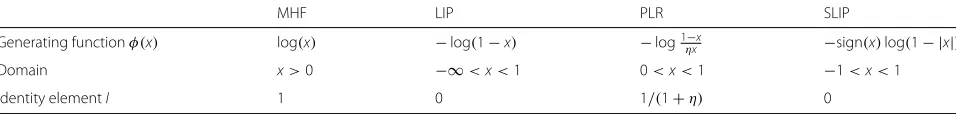
Prominent examples of generalized linear systems include the multiplicative homomorphic filter (MHF), the para-metric LR model, the LIP model, and the SLIP model. Key elements of these systems are summarized in Table 1.
Table 1Examples of generalized linear systems
MHF LIP PLR SLIP
Generating functionφ(x) log(x) −log(1−x) −log1−x
ηx −sign(x)log(1− |x|) Domain x>0 −∞<x<1 0<x<1 −1<x<1
Identity elementI 1 0 1/(1+η) 0
2.2 Generalized gamma correction
To develop the generalized gamma correction algorithm, let us rewrite the gamma correction as follows:
y=xγ
=exp(γlog(x)) =φ−1[γ φ(x)]
=γ ⊗x (17)
where x > 0, γ is a real number, and φ(x) = log(x). As such, the gamma correction is written as the scalar multiplication of a particular GLS which is the MHF.
The concept of the GLS provides a theoretical frame-work to generalize the gamma correction algorithm by using other generating functions. We will thus call the scalar multiplication operation of a GLS a generalized gamma correction. In the past, image enhancement using the scalar multiplication operation of the LIP model [5] and the PLR model [6] have been studied. In this work, we study the application of the SLIP model.
2.3 Generalized gamma correction using the SLIP model
The generalized gamma correction due the SLIP-based scalar multiplication is as follows:
y=γ ⊗x
=sign(x)1−(1x|)γ (18)
In Fig. 3c, d, we demonstrate the effects of setting dif-ferent values ofγ. Because in the SLIP model the signal is defined in the interval(−1, 1)and the gray-scale value of the image is usually in the interval(0, 1), a pre-processing step which maps the interval (0, 1) to (−1, 1) is thus required. Details of this mapping will be discussed in next section. After the mapping, the scalar multiplication using the SLIP model can be configured(γ <1)to enhance the dynamic range of both shadow and highlight areas at the cost of compressing the dynamic range of the mid-tone. It can also be configured(γ > 1) to enhance the dynamic range of an image with a narrow histogram at the cost of compression of the dynamic ranges of both shadow and highlight. This can be clearly seen in Fig. 3c, d.
In Fig. 3, we also demonstrate the main differences between different generalized gamma correction algo-rithms due to different generating functions. We can see that gamma correction (using MHF) can be configured
(γ < 1) to enhance the dynamic range of the shadow
area at the cost of compression of that of the highlight area and vice versa(γ >1). The LIP scalar multiplication has a similar effect as that of gamma correction. Obvi-ously, these two algorithms are not capable of enhancing the dynamic ranges of the shadow and the highlight simul-taneously. The PLR model (defined in Table 1) has a parameter η (η > 0). In actual applications, it is eas-ier to indirectly specifyη by using the identity element of the vector addition operation denoted byI0 which is
given byI0 = (1+η)−1[6]. We can see from Fig. 3e, f
that setting different values ofI0leads to an
asymmetri-cal enhancement or compression effects on the shadow, mid-tone, and highlight areas. For example, whenγ <1, it will enhance the shadow or the highlight or both areas depending on the setting of the identity element. On the other hand, when γ > 1, it will enhance the dynamic range of the narrow histogram which can be centered at different pixel values which depend on the setting of the identity element.
3 Proposed algorithm
3.1 The general structure
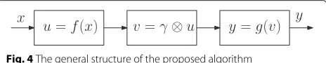
Let the input image to be processed be denoted asxand the final output image be denoted asy. Using the SLIP model, the signal set is defined asS = {x|x ∈ (−1, 1)}. Since after proper normalization, the gray scale of digi-tal images is in the interval (0, 1), the first step of using the proposed SLIP-based generalized gamma correction algorithm is to determine a function
u=f(x) (19)
such thatf :(0, 1)→(−1, 1). The second step is the appli-cation of the generalized gamma correction algorithm
v=γ ⊗u (20)
where v ∈ (−1, 1). The third step is to determine a function
y=g(v) (21)
such thatg:(−1, 1)→(0, 1). The general structure of the proposed algorithm is shown Fig. 4.
In the following, we definexmandxMas the minimum
and maximum values of the input imagex. We also define theρ-quantile value denoted byx(ρ)asPr(x<x(ρ))=ρ
wherexm ≤ x(ρ) ≤ xM and 0 ≤ ρ ≤ 1. In the limiting
cases, we havexm = x(ρ)|ρ=0andxM = x(ρ)|ρ=1. For
imagev, we also definevm,vM, andv(ρ)in the same way
as those corresponding terms in imagex.
3.2 Enhancing global low-contrast image 3.2.1 Determine the function f(x)
The dynamic range of the image can be defined as
Rx =x2−x1 (22)
wherex2 = x(ρ2)andx1 = x(ρ1). For example, we can
setρ2= 0.995 andρ1= 0.005 such that 99 % of the
pix-els are in the interval [x1,x2]. Since images of global low
Fig. 4The general structure of the proposed algorithm
contrast usually have a narrow histogram, one way to map the interval(0, 1)to(−1, 1)is by using
u=f(x)=x−b (23)
wherexm < b < xM. As such, we haveu1 = x1−band
u2=x2−b.
To determine the parameterb, it is reasonable to assume that after the scalar multiplication the results are
v1=γ ⊗u1= −c (24)
and
v2=γ ⊗u2=c (25)
where c is a positive constant close to 1. As such, the dynamic range of the imagevis given by
Rv=v2−v1=2c (26)
This assumption ensures that the dynamic range of the image is increased after the scalar multiplication. Using Eqs. 24 and 25 and the generating function of the SLIP model, we can derive the following result:
b= x2+x1
2 (27)
3.2.2 Determine the gainγ
Referring to Fig. 3d, the enhancement of the image is through the scalar multiplication with γ > 1. Setting a larger value forγ will lead to more contrast enhancement. We leave this as a parameter for the user to adjust to achieve the desirable results.
3.2.3 Determine the function g(v)
The final output image is obtained by a simple linear mapping
y=g(v)= v−v(ρ1) v(ρ2)−v(ρ1)
(28)
where ρ1andρ2 are user-specified parameters with the
property 0 ≤ ρ1 ≤ ρ2 ≤ 1. One simple way to set
these two parameters is to use the minimumvmand the
maximumvMinstead ofv(ρ1)andv(ρ2).
3.3 Enhancing local low-contrast image 3.3.1 Determine the function f(x)
We assume that the local low-contrast image has a broad histogram such as the one shown in Fig 1. We determine the mapping function f(x) based on the following con-siderations. Referring to Fig. 3c, in order for the scalar multiplication to effectively expand the dynamic range of the image content in both the shadow and highlight areas, the functionf(x)should have the property thatf(xm) =
−candf(xM) = c, wherec > 0 andcis a constant very
close to 1, e.g.,c = 0.999. As such, the gray-scale values in the shadow area are mapped to(−1,u1), whereu1<0
values in the highlight area are mapped to(u2, 1), where
u2>0 is an image-dependent constant. The center of the
mid-tone should be mapped to 0. We consider a linear mapping function
f(x)=a(x−b) (29)
When it satisfies the above conditions, it can be shown that
3.3.2 Determine the gainγ
Referring to Fig. 3c, since our goal is to enhance the dynamic ranges of the shadow and the highlight, the dynamic range of mid-tone has to be compressed. The gainγ can be determined by the amount of compression of the dynamic range of the mid-tone. More specifically, the mid-tone can be specified by the probabilityPr(|u|< u0) = ρ0. Once ρ0 (0 < ρ0 < 1) is specified,u0 can
be determined and the dynamic range [−u0,u0] will be
compressed based on a simple scalingv0 =τu0, whereτ
(0< τ <1) is the user-specified parameter. From Eq. 20, we can determine the scaling factor denotedγ0as follows:
v0=γ0⊗u0 (33)
In practice, as in most image processing software pack-ages, the user can directly specifyγ to achieve a desired outcome. However, obtaining γ using Eq. 34, the user can have more control over the trade-off between the compression of the mid-tone and the stretching of the dynamic ranges for the shadow and highlight.
3.3.3 Determine the function g(v)
For simplicity, we will adopt the same mapping function as that stated in Eq. 28.
3.4 Automatic enhancement
3.4.1 Image classification
In this section, we describe a simple method to classify an image as either global or local low contrast. The first task is to calculate the dynamic range of the input image using Eq. 22. If it is smaller than a predefined thresholdτ, i.e.,
Rx < τ, then the image is classified as global low
con-trast. IfRx ≥τ, then a further test is performed to see if
the image is of local low contrast. The assumption for the test is that a global low-contrast image usually has a uni-modal histogram while the local low-contrast image has a bimodal histogram. This assumption is justified from histograms of real images shown in Fig. 1.
The test is through the median absolute deviation (MAD)δ which is defined for a set of data{dn}n=1:N as
follows:
δ=median{|dn−τ|} (35)
where τ = median{dn} is the median of the data set.
The MAD is a robust measure of the spread of the data [36]. For an image, all pixels form a set of data denoted as {xn}n=1:N. We use Otsu’s method [37] to partition pixels
of the image into two sets:{un}n=1:Jand{vn}n=1::K, where J+K = N. We then calculate the MAD for the whole imageδ0, and the MAD for the two sets of pixelsδuandδv.
The image is classified as local low contrast whenδ0>
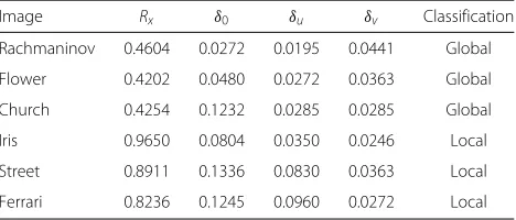
max(δu,δv). This classification rule is based on the obser-vation that for an image with a bimodal histogram, pixels can be robustly classified into two classes. The MAD of each class is usually smaller than the MAD of the whole image. The proposed classification method is confirmed in Table 2 which shows the values for images shown in Fig. 1.
3.4.2 Automatic enhancement
Once the low-contrast image is classified, the proposed algorithms developed in this paper can be applied. To enhance the global low-contrast image, the algorithm has one parameterγ (γ > 1) which can be set to a default valueγ =2. In actual application, the user can then adjust the value to achieve the desirable result. Similarly, the pro-posed algorithm for the local low-contrast image has one parameterγ (γ <1) which can be specified through the trade-off between the compression of the mid-tone and the expansion of the shadow and highlight. It can also be set to a default value, e.g., γ = 0.6. The user can then adjust the value to achieve the desirable result.
Table 2Image classification based on the dynamic range and median absolute deviation
Image Rx δ0 δu δv Classification Rachmaninov 0.4604 0.0272 0.0195 0.0441 Global
Flower 0.4202 0.0480 0.0272 0.0363 Global
Church 0.4254 0.1232 0.0285 0.0285 Global
Iris 0.9650 0.0804 0.0350 0.0246 Local
Street 0.8911 0.1336 0.0830 0.0363 Local
4 Results and comparison
For a color image, we first convert it from the RGB color space to the HSI space. The intensity component is pro-cessed. The result is then converted back to RGB space. For comparison, we have processed the image using the following algorithms in which the first two are classi-cal and well established, and the other three are recently published and have demonstrated good results.
• LCS: linear contrast stretching using MATLAB functionimadjustwith default settings
• CLAHE: contrast-limited adaptive histogram equalization [38] using MATLAB function
adapthisteqwith contrast parameter set to 0.004
• LCC: local color correction algorithm [7, 8] with default parameter settings1
• AGC: adaptive gamma correction2[9]
• PLR: parametric log-ratio model [6]
We use the standard deviation (σ), the mean (μ), and the entropy (H) of the intensity component as numeri-cal measures to compare images. The standard deviation has been used as an indicator of the contrast of the image [39]. The mean is used to measure the overall brightness of the image. The entropy is a measure of the flatness of the probability distribution of the gray-scale values in an image. When the distribution is a uniform distribution, the upper bound of the entropy of 8-bit is achieved for an image with gray-scale values quantized to 8 bits. Achieving higher entropy is one of the goals in image enhancement, e.g., histogram equalization [1]. However, it should be noted that none of these numeri-cal measures can replace the human subjective evaluation. The subjective evaluation depends on a lot of factors such as the viewing environment, the physical charac-teristics of the display device, and most importantly, the differences in viewer’s individual preference of contrast, sharpness, color, etc. As such, it is a subject currently under intense investigation and is out of the scope of this paper.
4.1 Enhancement of global low-contrast images
We use the Rachmaninov image to test the proposed algo-rithm. This image has a narrow histogram which is a typ-ical image of global low contrast. Referring to Section 3.2, we have tested three settings: γ = 2, 5, 7. Results are shown in Fig. 5 and in Table 3. From these results, we can make the following observations. Using the proposed algorithm, the standard deviation of the processed image increases with the increase of the parameter γ. Com-pared to the original image, the contrast of the processed image is significantly enhanced. This is confirmed visually
and numerically. Since the same image may appear to have different contrast on different display devices, the parameterγ can be set by the observer to produce a sat-isfactory result. The entropy of the processed images is also greater than that of the original image. This is an indication that the probability distribution of pixels in the processed image is closer to the uniform distribution than that of the original image.
Compared with the other algorithms, we can see that the proposed algorithm produces results visually quite close to that of the classical LCS. All algorithms tested, except the LCC algorithm, have improved the image qual-ity to some extent. This is confirmed from their respective values ofσ,μ, andH. The AGC also enhances the con-trast, but the overall brightness of the processed image is also increased. The CLAHE and PLR algorithms pro-duce similar results in which the enhancement in contrast is less than those produced by the proposed algorithm and the LCS. This is confirmed by the standard deviation of these images. The LCC algorithm increases the over-all brightness of the image, but it does not enhance the contrast of the image. As a result, the subjective quality of these images is not as satisfactory as that of the proposed algorithm and the LCS.
To further investigate the performance of the proposed algorithm, we run the same test using an overexposed flower image. It has a narrow histogram which is concen-trated in the highlight area. Results are shown in Fig. 6 and in Table 4. From these results, we can make very sim-ilar observations as those with the Rachmaninov image. Visually, the quality of the image produced by the pro-posed algorithm is similar to that produced by the PLR algorithm but is better than those of other algorithm tested.
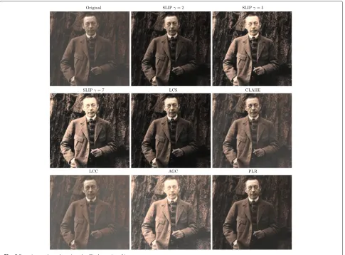
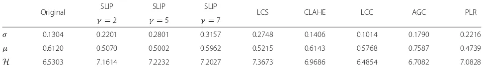
To demonstrate the robustness of the algorithm, we per-form experiment on the church image. We have tested three settings: γ = 2, 5, 7. Results are shown in Fig. 7 and in Table 5. From these results, we can clearly see that the low-contrast original image is due to haze-like effect rather than inaccurate exposure such as the flower image or the aging effect such as the Rachmaninov image. The proposed algorithm has successfully enhanced the con-trast of this image by removing the haze effect. Similar results have been achieved by using the linear contrast stretching. The numerical results shown in Table 5 sup-port these observations.
Overall, for the three test images, the proposed algo-rithm has produced images with the largest values of standard deviation and entropy among all algorithms tested.
4.2 Enhancement of local low-contrast images
Fig. 5Experimental results using the “Rachmaninov” image
the proposed algorithm (refer to Section 3.3) by setting
ρ0=0.1 andτ =0.5, by which the dynamic range of 10 %
of the pixels in the mid-tone will be compressed by a scal-ing factor of 0.5. To test the performance of the proposed algorithm with user-specifiedγ, we also setγ =1.2γ0and
γ =0.8γ0.
Results are shown in Fig. 8 and in Table 6. From these results, we can make the following observations. Using the proposed algorithm, the mean of the processed image increases with the increase of the parameter γ. This is an indication that the brightness of the shadow area
has been enhanced. The standard deviation of the pro-cessed image increases with the increase of ofγ but is always smaller than that of the original image. This is because the original image has an excessive contrast such that details in the shadow and highlight areas cannot be clearly seen. The proposed algorithm enhances the image by stretching the dynamic range of both areas towards the mid-tone. This results in a smaller standard devia-tion. The entropy of the processed image is roughly the same as that of the original image. Compared with the original image, the improvement in image quality can be
Table 3Comparison of the standard deviationσ, the meanμ, and the entropyHof the original and processed Rachmaninov images
Original SLIP SLIP SLIP LCS CLAHE LCC AGC PLR
γ=2 γ =5 γ=7
σ 0.0904 0.1439 0.2069 0.2348 0.1635 0.1299 0.0721 0.1800 0.1310
μ 0.3205 0.1789 0.2768 0.3152 0.1899 0.3277 0.4090 0.4645 0.2493
Fig. 6Experimental results using the over-exposed flower image
observed in both the shadow area (e.g., the leaves of the plant and the heater below the window) and the highlight area (e.g., the clouds in the sky). A negative effect of com-pressing the mid-tone can be observed in the part of the image where there are trees. Compared with the origi-nal image, the details of the trees in the processed image seem to be smoothed. This is because that part of the image is in the mid-tone and its dynamic range is com-pressed. This results in lost of contrast which leads to lost of details.
Compared with the other algorithms, we can see that the proposed algorithm produces results visually quite close to that of the LCC and PLR algorithms. The adaptive histogram equalization (CLAHE) significantly enhances the highlight area, but it does not enhance the shadow area. The AGC enhances the shadow area, but it does not enhance the highlight area. The classical linear contrast enhancement algorithm does not enhance both areas.
These observations can be explained from the standard deviation point of view. Refer to Table 6, the standard deviation of images produced by the LCS, CLAHE, LCC, and AGC algorithms is quite close to that of the original image. This indicates that these algorithms do not reduce the excess contrast of the original image. From the same point of view, we can understand that the quality of image produced by the PLR algorithm is similar to that pro-duced by the proposed algorithm, because the standard deviations are quite close to each other.
To further investigate the performance of the proposed algorithm, we process another image which is used in [9]. We test the proposed algorithm (refer to Section 3.3) by settingρ0=0.15 andτ =0.7, by which the dynamic range
of 15 % of the pixels in the mid-tone will be compressed by a scaling factor of 0.7. To test the performance of proposed algorithm with user-specifiedγ, we also setγ =1.2γ0and
γ =0.8γ0.
Table 4Comparison of the standard deviationσ, the meanμ, and the entropyHof the original and processed flower images
Original SLIP SLIP SLIP LCS CLAHE LCC AGC PLR
γ =2 γ=5 γ=7
σ 0.1073 0.2345 0.2841 0.3072 0.2289 0.1487 0.1364 0.0988 0.2502
μ 0.9059 0.8062 0.7517 0.7256 0.7654 0.8632 0.8644 0.9408 0.7787
Fig. 7Experimental results using the church image
Results are shown in Fig. 9 and in Table 7. From these results, we can make the following observations which are quite similar to those with the “iris” image. Using the proposed algorithm, the standard deviation increases with the increase of the parameterγ. However,
similar to the case of the “iris” image, the standard devi-ation of the processed image is smaller than that of the original image. This is because the original image has an excessive contrast with dark shadow areas such as the street inside the building and bright highlight areas
Table 5Comparison of the standard deviationσ, the meanμ, and the entropyHof the original and processed church images
Original SLIP SLIP SLIP LCS CLAHE LCC AGC PLR
γ=2 γ =5 γ=7
σ 0.1304 0.2201 0.2801 0.3157 0.2748 0.1406 0.1014 0.1790 0.2216
μ 0.6120 0.5070 0.5002 0.5962 0.5215 0.6143 0.5768 0.7587 0.4739
Fig. 8Experimental results using the “iris” image
such as the sky. The proposed algorithm enhances the image by stretching the dynamic range of both areas towards the mid-tone. As a result, the details of the dark areas can be easily seen, while the contrast of the sky is preserved.
Compared with the other algorithms, we can see that the proposed algorithm produces results visually quite close to that of the LCC and PLR algorithms. This can be
explained from the standard deviation point of view, i.e., the standard deviation of these images are quite close to each other. The adaptive histogram equalization (CLAHE) significantly enhances the highlight area, but it does not enhance the shadow area. The AGC enhances the shadow area, but it does not enhance the highlight area. The classical linear contrast enhancement algorithm does not enhance both areas.
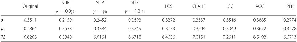
Table 6Comparison of the standard deviationσ, the meanμ, and the entropyHof the original and processed “iris” images
Original SLIP SLIP SLIP LCS CLAHE LCC AGC PLR
γ=0.8γ0 γ =γ0 γ =1.2γ0
σ 0.3511 0.2159 0.2452 0.2693 0.3272 0.3337 0.3516 0.3885 0.2774
μ 0.2864 0.3558 0.3384 0.3249 0.3133 0.3204 0.3049 0.3672 0.3578
Fig. 9Experimental results using the street image
To demonstrate the robustness of the proposed algo-rithm, we test it using the “ferrari” image3 which has a broad histogram. We set the parameters for the proposed algorithm as follows:ρ0=0.2 andτ =0.65. As such, the
dynamic range of 2 % of the pixels in the mid-tone will be compressed by a scaling factor of 0.65. To test the perfor-mance of the proposed algorithm with the user-specified
γ, we also setγ =1.2γ0andγ =0.8γ0, whereγ0is
deter-mined by the settingsρ0 = 0.2 and τ = 0.65. Results
are shown in Fig. 10 and Table 8. From this figure, we can clearly see that the results from the proposed algorithm
are similar to those produced by other algorithms. In fact, whenγ = γ0, the proposed algorithm is able to achieve
a good balance between retaining the contrast of the sky and enhancing the contrast of the bonnet of the car.
For the above three test images, the entropy of the pro-cessed images by all algorithms is about the same as that of the original image. This is because these test images have broad histograms and the aim of the proposed algo-rithm is not to further broaden the histogram. As such, the entropy of the processed image does change much from that of original image. In contrast, a global low-contrast
Table 7Comparison of the standard deviationσ, the meanμ, and the entropyHof the original and processed “street” images
Original SLIP SLIP SLIP LCS CLAHE LCC AGC PLR
γ=0.8γ0 γ=γ0 γ=1.2γ0
σ 0.2909 0.2063 0.2345 0.2578 0.2936 0.2853 0.2261 0.3410 0.2641
μ 0.3126 0.3653 0.3474 0.3329 0.3500 0.3939 0.3936 0.4416 0.3940
Fig. 10Experimental results using the ferrari image
image has a narrow histogram. As a result of enhancement of the dynamic range of the image, the proposed algorithm broadens the histogram leading to increase in entropy.
5 Conclusions
In this paper, based on the concept of the generalized linear system (GLS), we first proposed the generalized gamma correction algorithm as the scalar multiplication of a GLS. We then proposed an image enhancement algorithm by using the recently developed symmetric LIP (SLIP) model. We show that the proposed can be configured to effectively and efficiently enhance images of
either global low contrast or local low contrast. While the classical gamma correction algorithm can only enhance underexposed or overexposed images, the generalized gamma correction algorithm can be used to enhance images with low contrast in areas of shadow, mid-tone, highlight, or a combination of them. The expansion of the capability of the gamma algorithm thus constitutes a novel contribution of this paper. Experimental results and comparisons with classical and recently developed image enhancement algorithms demonstrate that the proposed generalized gamma correction algorithm is an effective tool.
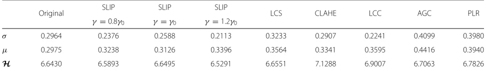
Table 8Comparison of the standard deviationσ, the meanμ, and the entropyHof original and processed “ferrari” images
Original SLIP SLIP SLIP LCS CLAHE LCC AGC PLR
γ =0.8γ0 γ=γ0 γ=1.2γ0
σ 0.2964 0.2376 0.2588 0.2113 0.3233 0.2907 0.2241 0.4099 0.3980
μ 0.2975 0.3238 0.3126 0.3396 0.3564 0.3341 0.3595 0.4416 0.3940
Endnotes
1The LCC algorithm is run remotely from the web site
http://www.ipol.im/pub/art/2011/gl_lcc/
2The source code is kindly provided by the authors. 3Available from http://www.ipol.im/pub/art/2011/gl_
lcc/#
Competing interests
The author declares that he has no competing interests.
Received: 5 November 2015 Accepted: 27 May 2016
References
1. RC Gonzalez, RE Woods,Digital Image Processing, (3rd Edition). (Prentice-Hall, Inc., Upper Saddle River, NJ, USA, 2006)
2. EH Land, JJ McCann, Lightness and the retinex theory. J. Opt. Soc. Am.61, 1–11 (1971)
3. R Kimmel, M Elad, D Shaked, R Keshet, I Sobel, A variational framework for retinex. Int. J. Comput. Vis.52, 7–23 (2003)
4. L Wang, L Xiao, H Liu, Z Wei, Variational Bayesian method for retinex. IEEE Trans. Image Process.23, 3381–3396 (2014)
5. M Jourlin, J-C Pinoli, Image dynamic range enhancement and stabilization in the context of the logarithmic image processing model. Signal Process.41, 225–237 (1995)
6. G Deng, Parametric generalized linear system based on the notion of the t-norm. IEEE Trans. Image Process.22(7), 2903–2910 (2013)
7. N Moroney, inIS&T/SID 8th Color Imaging Conference. Local color correction using non-linear masking (IS&T/SID, Scottsdale, Arizona, 2000), pp. 108–111
8. JGG Salas, JL Lisani, Local color correction. Image Process. On Line (2011). http://www.ipol.im/pub/art/2011/gl_lcc/
9. SC Huang, FC Cheng, YS Chiu, Efficient contrast enhancement using adaptive gamma correction with weighting distribution. IEEE Trans. Image Process.22(3), 1032–1041 (2013)
10. AV Oppenheim, RW Schafer, Jr Stockham TG, Nonlinear filtering of multiplied and convolved signals. IEEE Trans. Audio Electroacoustics. 16(3), 437–466 (1968)
11. Jr. Stockham TG, Image processing in the context of a visual model. Proc. IEEE.60(7), 842–828 (1972)
12. I Pitas, A Venetsanopoulos, Nonlinear mean filters in image processing. IEEE Trans. Acoust., Speech, Signal Process.34(3), 573–584 (1986) 13. H Shvaytser, S Peleg, Inversion of picture operators. Pattern Recogn. Lett.
5(1), 49–61 (1987)
14. M Jourlin, J-C Pinoli, A model for logarithmic image processing. J. Microsc. 149, 21–35 (1988)
15. J-C Pinoli, A general comparative study of the multiplicative
homomorphic, log-ratio and logarithmic image processing approaches. Signal Process.58(1), 11–45 (1997)
16. G Deng, J-C Pinoli, Differentiation-based edge detection using the logarithmic image processing model. J. Math. Imaging Vis.8(2), 161–180 (1998)
17. G Courbebaisse, F Trunde, M Jourlin, Wavelet transform and lip model. Image Anal. Stereol.21, 121–125 (2002)
18. M Lievin, F Luthon, Nonlinear color space and spatiotemporal MRF for hierarchical segmentation of face features in video. IEEE Trans. Image Process.13(1), 63–71 (2004)
19. JM Palomares, J Gonzalez, ER Vidal, A Prieto, General logarithmic image processing convolution. IEEE Trans. Image Process.15(11), 3602–3608 (2006)
20. J-C Pinoli, J Debayle, Logarithmic adaptive neighborhood image processing (LANIP): introduction, connections to human brightness perception, and application issues. EURASIP J. Adv. Signal Process. 2007(Article ID 36 105), 22 (2007). doi:10.1155/2007/36105 21. K Panetta, E Wharton, S Agaian, Human visual system-based image
enhancement and logarithmic contrast measure. IEEE Trans. Syst. Man Cybern. B.38(1), 174–188 (2008)
22. K Panetta, EJ Wharton, SS Agaian, Logarithmic edge detection with applications. J. Comput.3, 11–19 (2008)
23. H Gouinaud, Y Gavet, J Debayle, J-C Pinoli, inProc. 7tn Int. Symposium on Image and Signal Processing and Analysis. Color correction in the framework of color logarithmic image processing (IEEE, Dubrovnik, Croatia, 2011), pp. 129–133
24. M Jourlin, J Breugnot, F Itthirad, M Bouabdellah, B Close, inAdvances in Imaging and Electron Physics, ed. by PW Hawkes. Logarithmic image processing for color images, vol. 168 (Elsevier, 2011), pp. 65–107 25. JC Pinoli, J Debayle, Adaptive generalized metrics, distance maps and
nearest neighbor transforms on gray tone images. Pattern Recognit. 45(7), 2758–2768 (2012)
26. M Jourlin, E Couka, B Abdallah, J Corvo, J Breugnot, Asplünd’s metric defined in the logarithmic image processing (LIP) framework: a new way to perform double-sided image probing for non-linear grayscale pattern matching. Pattern Recognit.47(9), 2908–2924 (2014)
27. G Deng, An entropy interpretation of the logarithmic image processing model with application to contrast enhancement. IEEE Trans. Image Process.18(5), 1135–1140 (2009)
28. L Sbaiz, Y Feng, E Charbon, S Susstrunk, M Vetterli, inProc. IEEE Int. Conf. on Acoustics, Speech and Signal Processing. The gigavision camera (IEEE, Taiwan, 2009), pp. 1093–1096
29. G Deng, A generalized logarithmic image processing model based on the giga-vision sensor model. IEEE Trans. Image Process.3, 1406–1414 (2012) 30. SC Nercessian, K Panetta, SS Agaian, Multiresolution decomposition
schemes using the parameterized logarithmic image processing model with application to image fusion. EURASIP J. Adv. Signal Process.2011, Article ID 515084 (2011). doi:10.1155/2011/515084
31. V Patrascu, inIEEE Int. Conf. on Fuzzy Systems. Fuzzy enhancement method using logarithmic models (IEEE, Budapest, 2004), pp. 1431–1436 32. C Vertan, A Oprea, C Florea, L Florea, inAdvanced Concepts for Intelligent
Vision Systems. A pseudo-logarithmic image processing framework for edge detection (Springer, Juan-les-Pins, France, 2008), pp. 637–644 33. L Navarro, G Deng, G Courbebaisse, The symmetric logarithmic image
processing model. Digital Signal Process.23(5), 1337–1343 (2013) 34. G Deng, A generalized unsharp masking algorithm. IEEE Trans. Image
Process.20(5), 1249–1261 (2011)
35. R Vorobel, inProc 2010 Int. Kharkov Symposium on Physics and Engineering of Microwaves, Millimeter and Submillimeter Waves. Logarithmic type image processing algebras (IEEE, Kharkiv, Ukraine, 2010), pp. 1–3 36. DC Hoalin, F Mosteller, JW Tukey,Understanding Robust and Exploratory
Data Analysis. (John Wiley & Sons, 1983)
37. N Otsu, A threshold selection method from gray-level histograms. IEEE Trans. Syst., Man, Cybern.9, 62–66 (1979)
38. K Zuiderveld, ed. by PS Heckbert. Graphics Gems IV, ch. Contrast Limited Adaptive Histogram Equalization (Academic Press Professional, Inc., San Diego, CA, USA, 1994), pp. 474–485
39. E Peli, Contrast in complex images. J. Opt. Soc. Am. A.7, 2032–2040 (1990)
Submit your manuscript to a
journal and benefi t from:
7Convenient online submission 7Rigorous peer review
7Immediate publication on acceptance 7Open access: articles freely available online 7High visibility within the fi eld
7Retaining the copyright to your article