Solution of Game Theory Problems by New Approach

Volume 8, No. 5, May-June 2017

International Journal of Advanced Research in Computer Science RESEARCH PAPER

Available Online at www.ijarcs.info

ISSN No. 0976-5697

Solution of Game Theory Problems by New Approach

Kalpana Lokhande

Department of Mathematics Priyadarshani College of Engineering

Nagpur (M.S.), India

P. G. Khot

Department of Statistics

MJP Educational Campus, RTM Nagpur University Nagpur (M.S.), India

N. W. Khobragade

Department of Mathematics

MJP Educational Campus, RTM Nagpur University Nagpur (M.S.), India

Abstract: In this paper, an alternative approach to the Simplex method for game theory problem is suggested. Here we proposed a new approach based on the iterative procedure for the solution of a game theory problem by alternative simplex method. The method sometimes involves less or at the most an equal number of iteration as compared to computational procedure for solving NLPP. We observed that the rule of selecting pivot vector at initial stage and thereby for some NLPP it takes more number of iteration to achieve optimality. Here at the initial step we choose the pivot vector on the basis of new rules described below. This powerful technique is better understood by resolving a cycling problem.

Keywords: Optimum solution, New method, Game theory Problem , operations research, no saddle point

INTRODUCTION

Game theory attempts to study decision-making in the situations where two or more intelligent and the rational opponents are involved under conditions of conflict and cooperation. The approach of the game theory is to seek to determine a rival’s most profitable counter-strategy to one’s own ‘best’ moves and to formulate the appropriate defensive measures.

Game theory is the formal study of conflict and cooperation. Game theoretic concepts apply whenever the actions of several agents are interdependent. These agents may be individuals, groups, firms, or any combination of these. The concepts of game theory provide a language to formulate structure, analyze, and understand strategic scenarios. In practical life, it is required to take decision in a competing situation when there are two or more opposite parties with conflicting interests and the outcome is controlled by the decision of the all parties concerned. Such problems occur frequently in the economics, Business, Administration Sociology, Political Science and Military training. It is in this context that the game theory was developed in the twentieth century. However the mathematician treatment of the Game Theory was made available only in 1944, when John-Von-Newmann and the Oscar Morgenstrem [15] published their article ‘Theory of the Game and Economics behaviour. The Von-Newmann’s approach to solve the Game theory problems was based on the maximum losses. Most of the problems can be handled by this principle.

In 1994, B¨orgers' [1] discussed the theory of Weak Dominance and Approximate Common Knowledge. Brown [2]studied Iterative Solution of Games by Fictitious Play in Activity Analysis of Production and Allocation. Dantzig [3]discussed Maximization of linear function of variables subject to linear inequalities. Fudenberg and Levine [4] studied The Theory of Learning in Games. Gass [5]discussed Linear Programming. Ghadle, Pawar and Khobragade [6] find the Solution of Linear Programming

Problem by New Approach. Khobragade and Khot [7] discussed Alternative Approach to the Simplex Method and Lokhande, Khobragade, Khot[8] studied Simplex Method: An Alternative Approach. O'Neill [9] discussed Non metric Test of the Minimax Theory of Two-person Zero-sum Games.

Rasmussen [10] studied Games and information: an introduction to game theory. Sharma [11] has written the book on Operation Research. Stinchcombe [12] discussed General Normal Form Games. Tang [13] studied Anticipatory Learning in Two-person Games: Some Experimental Results. Vaidya, Khobragade [14] found the Solution of Game Problems Using New Approach. Weibull [16] studied Evolutionary Game Theory.

In this paper, an attempt has been made to solve the game theory problems by KKL method.

ALGORITHMOFKKLMETHOD

Step 1. For the m×nrectangular game when either m or n or both are greater than equal to three, new linear programming approach is as follows:

Let the two person zero sum game be defined as follows: Player A has m course of action

(

)

m

A A

A₁, ₂,..., and player B has n course of the action

(

)

n

B B

B₁, ₂,..., . The pay-off to the player A if he selects strategy Ai and player B select

j

B is aij. Mixed strategy for player A is defined by the probabilities

m

p

p

,...,

1 , where

p

1

+

...

+

p

m

=

1

and mixed

strategy for player B is defined by

n

q

q

,...,

1 where

1

...

1

+

+

q

n

=

q

.

Player A

Minimize

ν

1

=

Z or

y

1

+

y

2

+

...

.

y

n Subject to the constraints:

1

...

...

1 2 12 1

11

y

+

a

y

+

a

n

y

n

≥

a

1

...

...

2 2 22 1

21

y

+

a

y

+

a

n

y

n

≥

a

1 ... ... .... ... ... ... ... ... .... ... ... ... ... ... 2 2 1

1 + m + mn m ≥

m y a y a y

a Player B Maximize ν 1 =

Z or x1+x2+...xn Subject to the constraints:

1 ... ... 1 2 12 1

11x +a x +anxn ≤

a 1 ... ... 2 2 22 1

21x +a x +a nxn ≤

a 1 ... ... .... ... ... ... ... ... .... ... ... ... ... ... 2 2 1

1 + m + mn m ≤

m x a x a x

a

The steps for the computation of the optimal solution are as follows:

Step 2: Formulate the linear programming model of the real world problem that is obtained a mathematical representation of the problems objective function and constraints as stated below.

Maximize

M

=

c

1

x

1

+

c

2

x

2

+

...

+

c

n

x

n Subject to constraints:

1 1

2 12 1

11

x

a

x

...

a

x

b

a

+

+

+

_{n n}

≤

2 2

2 22 1

21x a x ... a x b

a + + + _{n n} ≤

m n n m m

m

x

a

x

a

x

b

a

+

+

...

+

≤

...

...

...

...

...

...

...

...

...

...

...

...

2 2 1 1

x1,x2,x3,...,xn ≥0

If the objective function is minimized, then convert it into a problem of maximizing by using the rule

Minimum M= - (Maximum (-M))

Allbi′s,i=1,2,...,m must be non negative. If any one of

bi

is negative, multiply corresponding inequality by (-1), So as to get allbi′s,

i

=

1

,

2

,...,

m

non-negative.

Step 3: Convert all inequations of the constraints into the equations by introducing slack variables in the left hand side of constraints and assign a zero coefficient to the corresponding variable in the objective function. Thus we can reformulate the problem in terms of equation as follows: Maximize

m n

nx p p p

c x

c x c

M= _{1 1}+ _{2 2} +...+ +0 ₁+0 ₂+...+0 Subject to constraints:

a

11

x

1

+

a

12

x

2

+

...

+

a

1n

x

n

+

p

1

=

b

1 a₂₁x₁+a₂₂x₂ +...+a_2nx_n +p₂ =b₂

m m n n m m

m

x

a

x

a

x

p

b

a

+

+

...

+

+

=

...

...

...

...

...

...

...

..

...

...

...

...

...

...

2 2 1 1

wherex₁,x₂,x₃,...,x_n ≥0 and 0

.., ,... , , _{2 3}

1 p p pm ≥

p

Step 4: An initial basic feasible solution is obtained by setting

x

₁

=

x

₂

=

x

₃

=

...

=

x

_n

=

0

. Thus we get

1 1 b

p = ,p2 =b2,…, pm =bm.

Step 5: For computational, efficiency and simplicity, the initial basic feasible solution, the constraint of the standard linear programming problem as well as the function can be displayed in a tabular form,

Reducing The Game Problem To A L.P.P.

It is somewhat more difficult to solve a game problem with an

m

×

n

payoff matrix having neither a saddle point nor any dominant column or row.

Further, in order to avoid any graphical simplification, we consider the general case when neither

m

nor

n

is 2. The problem is to determine

m

probabilities

p

_i for player A, say, with which he must mix his

m

pure strategies to get his mixed strategy,

n

probabilities

q

_j for player B, say, with which he should mix his

n

moves to get his mixed strategy; and the expected optimum value

v

of the game. Consider an

m

×

n

rectangular payoff matrix

(

a

_ij

)

for player A.

Let _

     = m m m p p A A S   1

1 _and

      = n n n q q B B S   1 1

where

∑

∑

= = = = m i n j j i q p 1 1

1, be the mixed strategies for the two players respectively.

Player A select

p

_i that will maximize his minimum expected payoff in a column, white player B selects the q_j that will minimize his maximum expected loss in a row of the payoff matrix (aij).

Now, the expected gains gj(j=12n) of player A against B’s moves are given by

m m p a p a p a

g1= 11 1+ 21 2++ 1

m m p a p a p a

g2 = 12 1+ 22 2++ 2



m mn n

n

n a p a p a p

g = _{1 1}+ _{2 2}++

and the expected losses

l

i

(

i

=

1

2



m

)

of player B against A’s moves are given by

n n

q

a

q

a

q

a

l

₁

=

_{11 1}

+

_{12 2}

+



+

₁

n nq a q a q a

l2= 21 1+ 22 2++ 2



n mn m

m

m a q a q a q

l + 1 1+ 2 2++ .

Thus, mathematically, minimax maximin principle suggests that player A should select p_i(p_i≥0,

∑

= = m i i p 1

1) that will yield _{max[min( )]}

j j

i g

for j=12n and the player B should select q_j(q_j≥0,

∑

= = n j j q 1 1) that will yield _{min[max( )]}

i i

j l

Let _{min( )}

j

j g

u= and

max

(

_i

)

i

l

v

=

,

then the problem for player A is to Maximize

u

subject to the constraints :

∑

=

≥

= m

i i

i p u

a g

1 1

1

∑

= =

m

i i

p 1

1 ,

∑

= ≥ = m

i i

i p u

a g

1 2

2 , pi ≥0 for all

i

.



∑

=

≥

= m

i i in

n a p u

g

1

and the problem for player B is to Minimize

v

subject to the constraints :

∑

= ≤ = n

j j

jq v

a l

1 1 1

∑

=

≤ = n

j j

jq v

a l

1 2

2 ,

∑

= =

n

j j

q 1

1



∑

=

≤

= n

j j mj

m a q v

l

1

, qj≥0 for all

j

.

The above LPP formulation can be simplified by assuming that

u

and

v

both are positive. For, every element of (a_ij) can be made strictly greater than zero by adding some constant to all the entries of

(

a

_ij

)

.

After the optimum solution is obtained, the true value of the game is obtained by subtracting that constant. Thus assuming that

u

>

0

,

v

>

0

, we introduce the new variables

u p

p i

i=

′

i

=

1

2



m

and v q

q′j = j , j=12n

so that the two problem become :

Problem of Player A

Maximize

u

= Minimize

∑

∑

= =

′

=

=

m

i i m

i i

p

u

p

u

1 1

1

i.e. Minimize

p

₀

=

p

₁

′

+

p

₂

′

+



+

p

_m

′

subject to the constraints :

1

1 2

21 1

11

p

′

+

a

p

′

+

+

a

m

p

′

m

≥

a



1

2 2

22 1

12

p

′

+

a

p

′

+

+

a

m

p

′

m

≥

a





1

2

2 1

1n

p

′

+

a

n

p

′

+

+

a

mn

p

′

m

≥

a



0 ≥ ′

i

p ,

i

=

1

2



m

Problem of Player B

Minimize v=maximize

∑

∑

= =

′ =

= n

j j n

j j

q v q

v 1 1

1

i.e. Maximize q0=q1′+q′2++q′_n Subject to the constraints :

1 1 2

12 1

11q′+a q′+ +anq′n≤

a 

1 2 2

22 1

21q′+a q′+ +a nq′n≤

a 



1 2

2 1

1 ′+ m ′+ + mn ′n≤

mq a q a q

a 

0

≥ ′_j

q , j=12n.

After the optimum solution is obtained using the new simplex method, the original optimum values can be determined.

Notice that B’s problem is actually the dual of A’s problem. Thus if one problem is solved, that will automatically yield the solution to the other.

Example1: Solve the following 3×3 game by linear programming:

Player B Player A

1 –1 –1

–1 –1 3

–1 2 –1

Solution: The given payoff matrix does not possess a saddle point. Since the maximin value is (–1), it is possible that the value of the game may be non – positive. Thus a constant

1

≥

C is added to all the elements of the payoff matrix.

Let C=2, the payoff matrix then becomes Player B

Player A

3 1 1

1 1 5

1 4 1

The problem of player A is to determine p₁, p₂ and p₃ so as to

Minimize

3 2 1 0

1

p p p u

p = = ′+ ′+ ′ Subject to the constraints :

1

3

p

₁

′

+

p

₂

′

+

p

₃

′

≥

1 4 3 2 1′+p′+ p′≥

p

1 5 2 3 1′+ p′+p′≥

p ,

0

,

,

2 3 1

′

p

′

p

′

≥

p

where _;

u p

p i

i=

′ u= minimum expected gain of A. The problem of player B is to determine

q

₁

,

q

₂

,

q

₃ so as to Maximize

3 2 1 0

1

q q q v

q = = ′+ ′+ ′ subject to the constraints :

1 3q1′+q2′+q3′ ≤

1 5 ₃ 2 1′+q′+ q′≤

q

1 4 2 3 1′+ q′+q′≤

q ,

0

,

,

2 3 1

′

q

′

q

′

≥

q

.

where v q

[image:4.595.88.510.71.224.2]

Table I. Initial Simplex Table

C = 1 1 1 0 0 0

B

C

y

_B

x

_B

y

₁

y

₂

y

₃

y

₄

y

₅

y

₆ Ratio

0

4

y

1 3 1 1 1 0 0 1/1

0

5

y

1 1 1 5 0 1 0 1/5

0

6

y

1 1 4 1 0 0 1 1/1

0 –1 –1 –1 0 0 0 Z_j−C_j

Ψj 4 6 7

↑ ↓

Here max [(_Zj−_Cj) + Ψj] is the entering vector, where

Ψ

=

∑

ij

j

a

.

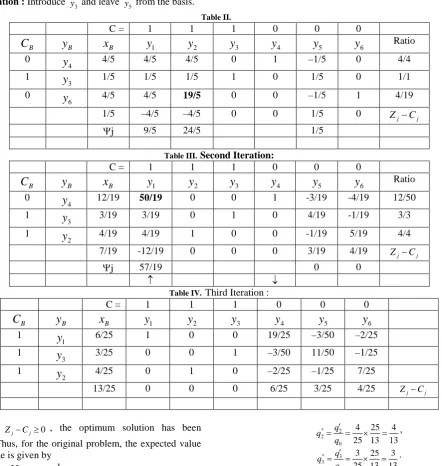
First Iteration : Introduce 3

y and leave y5 from the basis.

Table II.

C = 1 1 1 0 0 0

B

C

y

B

x

B

y

1

y

2

y

3

y

4

y

5

y

6 Ratio

0

4

y

4/5 4/5 4/5 0 1 –1/5 0 4/4

1

3

y

1/5 1/5 1/5 1 0 1/5 0 1/1 0

6

y

4/5 4/5 19/5 0 0 –1/5 1 4/19

1/5 –4/5 –4/5 0 0 1/5 0

j

j C

Z −

Ψj 9/5 24/5 1/5

Table III. Second Iteration:

C = 1 1 1 0 0 0

B

C

y

_B

x

_B

y

₁

y

₂

y

₃

y

₄

y

₅

y

₆ Ratio

0

4

y

12/19 50/19 0 0 1 -3/19 -4/19 12/50

1

3

y

3/19 3/19 0 1 0 4/19 -1/19 3/3

1

2

y

4/19 4/19 1 0 0 -1/19 5/19 4/4

7/19 -12/19 0 0 0 3/19 4/19 Z_j−C_j

Ψj 57/19 0 0

↑ ↓

Table IV. Third Iteration :

C = 1 1 1 0 0 0

B

C

y

B

x

B

y

1

y

2

y

3

y

4

y

5

y

6

1

1

y

6/25 1 0 0 19/25 –3/50 –2/25

1

3

y

3/25 0 0 1 –3/50 11/50 –1/25

1

2

y

4/25 0 1 0 –2/25 –1/25 7/25

13/25 0 0 0 6/25 3/25 4/25 Z_j−C_j

Since all Z_j−C_j≥0 , the optimum solution has been attained. Thus, for the original problem, the expected value of the game is given by

C q

v = −

0

* 1 ₂

13 25₋

=

13 1 − =

and the optimum mixed strategy for B is given by

13 6 13 25 25

6

0 1 *

1 = × =

′ =

q q

q ,

13 4 13 25 25

4

0 2 *

2 = × =

′ =

q q

q ,

13 3 13 25 25

3

0 3 *

3 = × =

′ =

q q

q .

The optimum strategies for A are obtained from the dual solution to the above problem.

The optimum values for p₁′,p₂′ and 3

p′, where u p

p i

i′=

) 3 2 , 1

[image:4.595.78.521.237.703.2]

above optimum simplex table under y₄ y₅ and y6, because A’s problem is the dual of B’s problem.

Thus 25

6

1′= p ,

25 3 2=

′

p , 25

4

3=

′

p ,

25 13

0 0=q =

p .

Hence the optimum mixed strategy for A is given by

13 6 13 25 25

2

0 1 *

1 =

           = ′ =

p p

p ,

13 3 13 25 25

3

0 2 *

2 =

           = ′ =

p p

p ,

13 4 13 25 25

4

0 3 *

3 =

           = ′ =

p p p

Hence the optimum solution to the original game problem is

   

  =

13 / 4 13 / 3 13 / 6

3 2

1 A A

A SA

,

   

  =

13 / 3 13 / 4 13 / 6

3 2

1 B B

B SB

,

13

1

*₌₋

v .

Example 2: Solve the following 3×3 game by linear programming:

Player B

Player A 8 9 3

2 5 6

4 1 7

1 4 1

Solution The problem of player A is to determine p₁, p2 and

3

p so as to Minimize

3 2 1 0

1

p p p u

p = = ′+ ′+ ′ Subject to the constraints:

1 4 2

8p₁′+ p₂′+ p₃′≥

1 5

9p1′+ p2′+p3′≥

1 7 6

3p1′+ p2′+ p3′≥ , 0 , , 2 3 1′ p′ p′≥ p

Where _;

u p

p i

i =

′ u= minimum expected gain of A. The problem of player B is to determine

3 2 1,q ,q

q so as to Maximize

3 2 1 0

1

q q q v

q = = ′+ ′+ ′ subject to the constraints :

1 3 9

8q1′+ q2′+ q3′≤

1 6 5

2q1′+ q2′+ q3′≤

1 7 4q₁′+q₂′+ q₃′≤ , q1′,q2′,q3′≥0. where

v q

q′_j = j ;

v

=

maximum expected loss of B.

Let us solve B’s problem by simplex method. Introducing the slack variable _q4′_,q5′_,q6′ respectively in the constraints of the problem, one obtains the following simplex tables :

Initial Simplex Table

C = 1 1 1 0 0 0

B

C

y

_B

x

_B

y

₁

y

₂

y

₃

y

₄

y

₅

y

₆ Ratio

0

4

y

1 8 9 3 1 0 0 1/3

0

5

y

1 2 5 6 0 1 0 1/6

0

6

y

1 4 1 7 0 0 1 1/7

0 –1 –1 –1 0 0 0 Zj−Cj

Ψj 14 15 16

↑ ↓

First Iteration : Introduce y₃ and leave 6

y from the basis.

C = 1 1 1 0 0 0

B

C

y

_B

x

_B

y

₁

y

₂

y

3

y

4

y

5

y

6 Ratio

0

4

y

4/7 44/7 60/7 0 1 0 -3/7 1/15

0

5

y

1/7 -10/7 29/7 0 0 1 -6/7 1/29

1

3

y

1/7 4/7 1/7 1 0 0 1/7 1

1/7 -17/7 22/7 -1 -1 -1 -6/7

j

j C

Z −

Ψj

↑ ↓

Second Iteration : Introduce 2

y and leave y4 from the basis

C = 1 1 1 0 0 0

B

C

y

_B

x

_B

y

₁

y

₂

y

₃

y

₄

y

₅

y

₆ Ratio

0

4

y

8/29 268/29 0 0 1 -60/29 39/29 12/50

1

2

y

1/29 -10/29 1 0 0 7/29 -6/29 3/3

1

3

13/29 321/29 0 0 0 66/2919 68/2919 Z_j−C_j

↑ ↓

Third Iteration : Introduce

y

₁ and leave

y

₄ from the basis

C = 1 1 1 0 0 0

B

C

y

B

x

B

y

1

y

2

y

3

y

4

y

5

y

6

1

1

y

2/67 1 0 0 29/68 -15/67 39/268

1

2

y

3/67 0 0 1 5/134 11/67 -21/134

1

3

y

8/67 0 1 0 -9/134 7/67 11/134

13/67 0 0 0 21/268 12/268 19/268

j

j C

Z −

Since all _{− ≥0}

j j C

Z , the optimum solution has been attained.

Thus, for the problem, the expected value of the game is given by

67 / 13 1

0

*= =

q v

and the optimum mixed strategy for B is given by

13 2 13 67 67

2

0 1 *

1 = × =

′ =

q q

q ,

13 3 13 67 67

3

0 2 *

2 = × =

′ =

q q

q ,

13 8 13 67 67

8

0 3 *

3 = × =

′ =

q q

q .

The optimum strategies for A are obtained from the dual solution to the above problem.

The optimum values for p₁′,p₂′ and p₃′ , where u p

p i

i=

′

) 3 2 , 1

(i=  are read off from the net evaluation row of the above optimum simplex table under y₄ y5 and y6, because A’s problem is the dual of B’s problem.

Thus _21/268 1′=

p , p2′=12/268, p3′=19/268, Hence the optimum mixed strategy for A is given by

52 21 13 67 268

21 0 1 *

1 =

           = ′ =

p p

p ,

52 12 13 67 268

12 0 2 *

2 =

           = ′ =

p p

p ,

52 19 13 67 268

19 0 3 *

3 =

           = ′ =

p p p

Hence the optimum solution to the original game problem is

   

  =

52 / 19 52 / 12 52 / 21

3 2

1 A A

A SA

,

   

  =

13 / 8 13 / 3 13 / 2

3 2

1 B B

B SB

,

13 67 *=

v .

Example3:. Solve the following

2

×

3

game by linear programming:

Player B

Player A 3 –1 4

6 7 -2

Solution : Since two of the entries in the pay-off matrix are negative a constant C≥1 is added to all the elements of the payoff matrix.

Let 3, the payoff matrix then becomes Player B

Player A 6 2 7

9 10 1

The problem of player A is to determine p₁, p2 and p3 so as to

Minimize

2 1 0

1

p

p

u

p

=

=

′

+

′

Subject to the constraints :

1

9

6

p

1

′

+

p

2

′

3

≥

1

10

2

p

1

′

+

p

2

′

3

≥

1

7

p

1

′

+

p

2

′

≥

,

0

,

2 1

′

p

′

≥

p

Where _;

u p

p i

i=

′ u= minimum expected gain of A. The problem of player B is to determine

q

₁

,

q

₂

,

q

₃ so as to Maximize

3 2 1 0

1

q q q v

q = = ′+ ′+ ′ subject to the constraints :

1

7

2

6

q

1

′

+

q

2

′

+

q

3

′

≤

1

10

9

q

1

′

+

q

2

′

+

q

3

′

≤

;

0

,

,

2 3 1

′

q

′

q

′

≥

q

.

where v q

q′j= j ; v= maximum expected loss of B.

Let us solve B’s problem by simplex method. Introducing the slack variable q₄′,q₅′,q₆′ respectively in the constraints of the problem, one obtains the following simplex tables :

Initial Simplex Table

C = 1 1 1 0 0

B

C

y

_B

x

_B

y

₁

y

₂

y

₃

y

₄

y

₅ Ratio

0

4

0

5

y

1 9 10 1 0 1 1/9

0 –1 –1 –1 0 0 Z_j−C_j

Ψj 15 12 8

↑

First Iteration : Introduce y₁and leave y₅ from the basis.

C = 1 1 1 0 0

B

C

y

_B

x

_B

y

₁

y

₂

y

₃

y

₄

y

₅ Ratio

0

4

y

1/3 0 -14/3 19/3 1 -2/3 1/19

1

1

y

1/9 1 10/9 1/9 0 1/9 1

1/9 1/9 -8/9 1/9

j

j C

Z −

Ψj 0 -2 39/9 0 -5/9

↑ ↓

Second Iteration : Introduce 1

yand leave y₅ from the basis

C = 1 1 1 0 0

B

C

y

_B

x

_B

y

₁

y

₂

y

₃

y

₄

y

₅ Ratio

1

3

y

1/19 0 -14/19 1 3/19 -2/19 -14

1

1

y

2/19 1 68/57 0 -1/57 7/57 3/34

0 11/57 0 -1/57 7/57

j

j C

Z −

Ψj 2 26/57 8/57 1/57

Third Iteration : Introduce 2

y

and leave 1

y

from the basis

C = 1 1 1 0 0

B

C

y

B

x

B

y

1

y

2

y

3

y

4

y

5 Ratio

1

3

y

2/17 42/68 0 1 5/34 -1/34 -14

1

2

y

3/34 57/68 1 0 -1/68 7/68 3/34

7/34 29/68 0 0 9/68 5/68

j

j C

Z −

Thus, for the original problem, the expected value of the game is given by

C q

v = −

0

* 1

3 7 34₋

=

7 13

=

and the optimum mixed strategy for B is given by

68

9

0 1 *

1

=

′

=

q

q

q

,

68

5

0 2 *

2

=

′

=

q

q

q

,

Hence the optimum solution to the original game problem is

   

  =

14 / 5 14 / 9

2

1 A

A SA

,

   

  =

7 / 4 7 / 3 0

3 2

1 B B

B SB

, 34

7 *=

v .

CONCLUSION

We observed that the solution of Game Theory problem has been obtained by our technique very easily and requires less or at the most equal number of iterations than traditional simplex method. This technique is very useful to apply on numerical problems, reduces the labour work, gives more accuracy and improved optimum solution. Therefore this method is more powerful in solving Game Theory problems as compare to traditional simplex method.

REFERENCES

[1] B¨orgers, “Weak Dominance and Approximate Common Knowledge,” Journal of Economic Theory, 64(1) 265-277, 1994.

[2] G. Brown, “Iterative Solution of Games by Fictitious Play," in Activity Analysis of Production and Allocation, John Wiley & Sons, New York.1951 .

[3] G. B. Dantzig, “Maximization of linear function of variables subject to linear inequalities” In: 21-Ed. Koopman Cowls Commission Monograph, 13, John Wiley and Sons, Inc., New Yark, 1951.

[4] D Fudenberg and D Levine, “The Theory of Learning in Games”, Boston: MIT Press,1998.

[5] S. I. Gass, “Linear Programming,” 3/e, McGraw-Hill Kogakusha, Tokyo ,1969.

[6] K. P. Ghadle, T. S. Pawar and N. W. Khobragade, “Solution of Linear Programming Problem by New Approach”, IJEIT, Vol.3, Issue 6. Pp.301-307, 2013

[7] N. W. Khobragade and P. G. Khot, “Alternative Approach to the Simplex Method-II”, Acta Ciencia Indica, Vol.xxx IM, No.3, 651, 2005.

[9] B. O'Neill, “Non metric Test of the Minimax Theory of Two-person Zero-sum Games”, Proceedings of the National Academy of Sciences, 84, 1987, 2106-2109.

[10] E. Rasmussen, “Games and information: an introduction to game theory”.

[11] S. D. Sharma, “Operation Research”, Kedar Nath Ram Nath, 132, R. G. Road, Meerut-250001 (U.P.), India.

[12] M. B. Stinchcombe, “General Normal Form Games. Working paper”, Department of Economics, University of Texas at Austin.169,2001.

[13] F. F. Tang, “Anticipatory Learning in Two-person Games: Some Experimental Results”, Journal of Economic Behavior and Organization, 44, 221-232,2001.

[14] N. V. Vaidya, N. W. Khobragade, “Solution of Game Problems Using New Approach”, IJEIT, Vol. 3, Issue 5, 2013. [15] Von Neumann and Morgenstern, “The Theory of Games and Economic Behavior”, Princeton: Princeton University Press, 1944.