Volume 9, No. 2, March-April 2018
International Journal of Advanced Research in Computer Science RESEARCH PAPER
Available Online at www.ijarcs.info
ISSN No. 0976-5697
RFKNN: ROUGH-FUZZY KNN FOR BIG DATA CLASSIFICATION
Mohamed Mahfouz
Ph.D., Department of Computer and Systems Engineering, Faculty of Engineering, University of Alexandria,
Alexandria, Egypt 21544, Egypt
Abstract: The K-nearest neighbors (kNN) is a lazy-learning method for classification and regression that has been successfully applied to several
application domains. It is simple and directly applicable to multi-class problems however it suffers a high complexity in terms of both memory and computations. Several research studies try to scale the kNN method to very large datasets using crisp partitioning. In this paper, we propose to integrate the principles of rough sets and fuzzy sets while conducting a clustering algorithm to separate the whole dataset into several parts, each of which is then conducted kNN classification. The concept of crisp lower bound and fuzzy boundary of a cluster which is applied to the proposed algorithm allows accurate selection of the set of data points to be involved in classifying an unseen data point. The data points to be used are a mix of core and border data points of the clusters created in the training phase. The experimental results on standard datasets show that the proposed kNN classification is more effective than related recent work with a slight increase in classification time.
Keywords: classification, kNN, big data, clustering, fuzzy sets, rough sets.
I. INTRODUCTION
The K-Nearest Neighbors (kNN) is a renowned data mining technique. It is applied to both classification and regression tasks in several application domains [1], [2]. Traditional kNN classification algorithm works as follows: A data point is classified by identifying the k neighbors of
this data point and counting the number of neighbors from each class. The data point is assigned to the class to which the majority of the k neighbors belong. k is a positive
integer, typically small and depends on the size and distribution of the input data. When k = 1, then the unseen
data point is assigned to the class of its nearest neighbor. In binary (two classes) classification problems, it is meaningful to choose k to be an odd number to avoid tied votes. One of
the key advantages of nearest neighbor approach is that the density function for each target data point is estimated locally and differently instead of being estimated once for the entire instance space [3]. From its definition, it is clear that it is simple (easy to implement), multi-class (can deal with datasets having more than two classes), memory-based (training set stored in memory without explicit generalization), and non-parametric method (no assumptions about the input data).
In [4], the performance of different similarity measures that can be used in the KNN algorithm, are evaluated. In [5], a new affinity function for distance measure between a test point and a training point based on local learning is introduced. A Bayesian method is investigated in [6] for estimating a proper value for k in kNN algorithm.
In [7], An adaptive parameter-free neighborhood construction algorithm based on density and connectivity is proposed to tackle the problem of estimating the set of neighbors for each data point without a priori information about the dataset. A recent approach in [8] proposed an algorithm termed CM-kNN that learns a correlation matrix to reconstruct test data points by training data to assign different k values to different test data points and applied the
proposed algorithm to regression and missing data imputation.
When traditional KNN decision rule is applied to unbalanced data, there is a tendency to assign an unseen object to the majority class label. Several strategies for selecting the objects to be dimmed from the majority class are proposed in [9]. Another approach is resizing the input dataset by either under sampling majority class, oversampling the minority class or by doing both at the same time (hybrid) [10], until the data is balanced.
Also, kNN is used in future selection as in [11] where a neighborhood rough set technique is used to rank and prioritize lists of potential tumor-related genes from the genetic profile. Other research studies that use an ensemble of KNN classifiers as a gene selector are found in [12] and [13].
Although the kNN algorithm has shown outstanding performance in a wide variety of problems, it lacks the scalability to manage (very) large datasets. The kNN suffers high computational complexity. The complexity to find the nearest neighbor training example of a single test instance is O(n·d), where n is the number of training objects and d is
the number of attributes (features). Also, an extra complexity O(k log k + n) to select the k closets neighbors.
Furthermore, the kNN model requires the training data to be stored in memory for a rapid computation of the distances. An example for early work for accelerating kNN is found in [1] where the fat k closest vectors are identified in the design
set of a kNN classifier for each input vector by performing a partial distance search in the wavelet domain.
However, early work does not suit very large datasets. This motivates researchers in the big data area to distribute the processing of a kNN classifier over a cluster of nodes to be suitable for the application of big data [14].
Landmark-based Spectral Clustering (LSC) is used in [17] for partitioning the input data. Landmarks for LSC are selected either randomly or using k-means and the corresponding techniques are termed as RC-kNN and LC-kNN respectively.
In this paper, we propose to integrate the principles of rough sets [18] and fuzzy sets [19] into the approach in [17]. This allows distinguishing between core and border objects in each produced cluster. In the classification of an unseen object, a proper set of data points are efficiently and effectively selected as a union of one core partition and several border partitions that are necessary for classifying the unseen data point depending on its membership in the clusters which are produced in the training phase. Two techniques are proposed termed as RC-RFkNN and LC-RFkNN for randomly or using k-means landmarks for LSC clustering respectively. Experimental results show that RC-RFkNN and LC-RC-RFkNN achieve an enhancement in terms of classification accuracy over RC-kNN and LC-kNN respectively.
The remainder of this paper is organized as follows. Section II details the proposed method along with the necessary background. Then, Section III presents the experimental setup and results with analysis of results. Finally, Section IV outlines the conclusions drawn in this work.
II. MATERIALS AND METHODS
A. Rough Set and Fuzzy Set
[image:2.595.54.263.561.684.2]Let a target set X to be represented using attribute subset P and P(X); P (X) are two crisp sets representing the lower boundary of X, and the upper boundary of the target set X respectively. The tuple <P(X),P (X)> composed of the lower and upper approximation of a set X
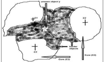
U is called a rough set [18]. In the remaining of this paper, we refer to the lower and upper approximation of a cluster Ci as L(Ci) and U(Ci) respectively. The lower approximation of a cluster L(Ci) is an unadventurous approximation consisting of only those objects which can definitely be identified as members of this cluster. The upper approximation includes all data points that might be members of the target set. (Some data points in the upper approximation may not be members of the target set).Figure 1 core and border regions of 3 overlapping clusters C1, C2 and C3, the borders of the 3 clusters should be included in predicting a label for y.
The lower approximation contains objects that are members of the target set with probability equals 1, while the upper approximation contains objects that are members of the target set with non-zero probability. As shown in Fig. 1, the boundary region, given by set difference U(Ci)-L(Ci) consists of those objects that can neither be ruled in nor
ruled out as members of the target cluster. A fuzzy set F [19] of U is a mapping from U into the unit interval [0, 1]: µF : U [0,1],
The crisp set that contains all the elements of U that have a nonzero membership value in F is called as the support of the fuzzy set F.
A function mapping of all the elements in a crisp set into real numbers in [0, 1] is called a membership function. The larger value of the membership function represents the higher degree of the membership. It means how closely an element resembles an ideal element. Membership functions can represent the uncertainty using some particular functions. In the following sections Border(Ci) refers to U(Ci)-L(Ci) while Core(Ci) refers to L(Ci).
B. Soft Clustering
The algorithm k-means [20] which is used in [17] as the final step for partitioning the input big dataset always results in memberships {0,1}. In the proposed algorithm we need fuzzy memberships i.e. positive grades of membership uij for
each object xj in cluster i. If we use fuzzy clustering
algorithm such as fuzzy k-means [21], an object may belong to all clusters with varying degree of belongingness. The pitfall is that all memberships are used in computing new centers which in turn used in computing new memberships at each iteration of the algorithm and hence small memberships still have an effect on the whole process. Furthermore, in the proposed algorithm we are interested in objects that have enough high membership to be considered core or border objects.
In [22] three mathematical models for soft clustering (semi-fuzzy) along with three algorithms for implementing them are introduced. The First model limits the fuzziness to a smaller subset of the available clusters. The second and third models allow a pattern to be associated with the proper number of clusters based on a proper choice of threshold value on distance or membership respectively. The concept of semi-fuzzy clustering are applied to several problems in bioinformatics [23], [24], [25]. In this paper the third model of soft (semi-fuzzy) clustering introduced in [22] will be applied instead of the k-means in [17].
C. RC-kNN and LC-kNN algorithms [17]
The most related technique for the proposed technique is a recent approach for scaling KNN in [17] which is based on Landmark-based Spectral Clustering (LSC). LSC starts by computing p landmarks by using the resulting centers of
running the k-means algorithm several times (or by using random sampling). Then, constructs an affinity matrix W between data points and landmark samples. The v
representative samples are computed using the eigenvectors of a matrix derived from W. The overall time complexity for LSC is O (p3+p2n). For each test sample, its nearest cluster
center is identified and its corresponding cluster is used as the new training dataset for this sample.
D. Proposed Algorithm
Table 1 describes the pre-classification steps of the proposed algorithm. Steps 1-4 in Table 1 represent the steps of LSC algorithm which are the same as in [17]. After computing p landmarks in step 1, r nearest landmarks for
each object xi are identified, denoted Z<i>. A matrix W of
r Z z l i j i ji i l h z x h z x w 2 2 2 2 2 / || || 2 / || || (1)Let W'= D-0.5 W where D is the row sum of W. Note that each column of W sums up to 1 and thus the degree matrix of W'W'T is I.
The matrix V in step 4 is called as right singular vectors of the k eigenvectors of W'W'T. V can be computed as follows:
1
'
W U VT T
(2) Where U= [u1, u2, ..., um] is called as the left singular vectors of the first k eigenvectors of W'W'T
In step 5, soft k-means is applied instead of k-means
Table 1 Proposed Pre-Classification Steps (Partitioning Process) Input:
X: dataset of n data points x1; x2;ڮڮ; xn
p: no. landmarks
m: number of clusters Output: m clusters; begin
1. Produce p landmarks using k-means or random sampling on X. 2. Compute matrix W as in Eq. (1).
3. Compute the first k eigenvectors of W'W'T, denoted by
U= [u1, u2, ..., um].
4. Compute V=[v1, v2, ..., vm] according to Eq. (2).
// each row in V is a data point
5. Apply soft k-means [22] on V to get m clusters
6. foreach cluster Ci identify Core(Ci) and Border(Ci) endfor end
The third model of [22] is used in step 5 in Table 1 instead of k-means. Soft k-means is similar to fuzzy k-means, except, in each iteration the computed memberships are compared to a threshold and any membership less than the specified threshold is set to zero and the memberships are re-normalized. We did a small modification to this model such that any membership is compared to the maximum membership if it less than the maximum by more than a threshold δ then it is set to zero and the memberships are re-normalized. The membership of an object y in a cluster j
denoted µj(y) is calculated as follows:
) 1 /( 1
1 ( , )
) , ( ) (
m m i i j j C y s C y s y (3)Where s(y,Cj) is the similarity between object y and the center of cluster Cj, m is a fuzzifier greater than 1. If
dissimilarity measure such as Euclidian distance were used then s(y,Cj) may be replaced by 1/ d(y,Cj).
In the proposed algorithm RFkNN, each cluster is represented by a crisp lower approximation (Core(Ci), and a fuzzy boundary (Border(Ci) ) see Fig. 1. As shown in Table 2, which describes the classification algorithm, after computing the memberships for the unseen data point in each cluster, then the membership values are sorted, and the difference of the two highest memberships is compared with a threshold value δ.
Let µij and µkj be the highest and second highest
memberships of subsequence xj.
If µij - µkj > δ, then xj Core(Ci) as well as xj
Border(Ci), xj
Border(Ck) for any cluster k≠i; and NewXis set to cluster Ci (both the core and border of Ci) otherwise,
NewX is set to cluster Ci (both the core and border of Ci) union the border of any cluster Ck such that µij - µkj < δ.
[image:3.595.307.557.113.353.2]Finally, in step 4, only the set of data points NewX is used in classifying the unseen data point y. That is, the proposed algorithm separates the core and overlapping portions of each cluster based on the threshold value δ.
Table 2: Proposed Classification Process Input:
X: the dataset X partitioned into m clusters denoted C1..Cm
y : a test (unseen) sample
δ : a threshold used for distinguishing border and core objects Input: y is an unseen object, k is the no. of nearest neighbors Output: The predicted class label for y
Begin
1. compute the fuzzy membership of y in each cluster Cj
denoted µj(y), j=1,2,…,m using Eq. (3)
2. set NewX = Core(Cj ) where arg max ( ) 1 y j j m j
3. fori=1 to m //Border(Cj) is always included
if (µj(y)- µi(y)) < then // default value for δ=0.15
NewX = NewX
Border(Ci) endif endfor4. apply kNN using NewX to predict a class label for y End
III. EXPERIMENTAL RESULTS
A. Input Data
[image:3.595.307.567.457.521.2]As mentioned in the previous sections, our proposed algorithm is an extension of RC-kNN and LC-kNN. Thus, in order to show the effectiveness of LC-RFkNN and RC-RFkNN algorithms, we took the kNN as the baseline and made a comparison between kNN, kNN, RC-kNN, LC-RFkNN and RC-LC-RFkNN using three large multi-class datasets listed in table 3 from UCI [26] and LIBSVM [27].
Table 3 Description of datasets used in our experiments
Dataset Name Ref. no. objects no. futures
LETTER [26] 20000 16
PENDIGITS [26] 10992 16
USPS [27] 7,291 256
B. Performance Measure
In the following experiments, the empirical accuracy is used for estimating the quality of the proposed classifier. Let g be a classifier, and xi and yi be respectively a test
sample and its class label. Let g(xi) be the predicted class for
xi using the classifier g. The accuracy can be calculated as
follows:
n i y xg i i
n Accuracy
1 ( )
1 1
(4) The accuracy in Eq. (1) is calculated as total number of corrected prediction divided by the total number of data points to be classified. Computing the accuracy on imbalanced data using Eq. (1) is a misleading performance measure.
n i y x g yi i iw n Accuracy 1 ) ( 1 1 (5) where wy be the weight of the class y as follows:
wy =
n i y yi n 1 1 / 1 (6)
performance measures can be easily computed as macro and micro average over all classes. TPi refers to the number of
instances of class i that are correctly classified as class i. FPi
is the number of instances of class j (i ≠ j) that are
incorrectly classified as class i. FNi is the number of
instances of class i that are incorrectly classified as class j (i
≠j). In order to be able to compare with RC-kNN and
LC-kNN, the accuracy is used in evaluating RFkNN as it was the only measure used in [17] .
C. Experimental results for different value of m As mentioned before the proposed algorithms RC-RFkNN and LC-RC-RFkNN are based on partitioning the datasets into several clusters. Each cluster in the proposed algorithm is seen as two crisp partitions core and border. The no. of clusters m is very important to the proposed
algorithm as it was very important to RC-kNN and LC-kNN algorithms [17].
The value of m directly affects the classification time and
accuracy. Thus, in order to select a proper value of m, a
group of experiments were conducted on the three standard datasets listed in table 3. By choosing different values of m
for RFkNN and RC-RFkNN. Specifically, the LC-RFkNN and RC-LC-RFkNN in this group of experiments were carried out on the three datasets with m=10, 15, 20, 25 and
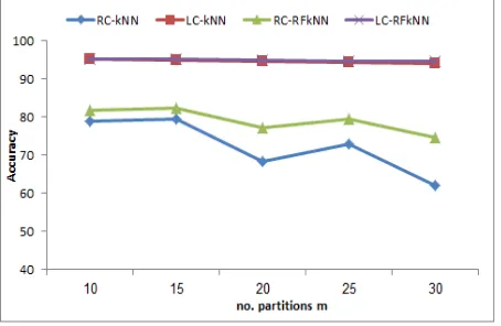
30, respectively as shown in Fig. 2-4. The values plotted for RC-kNN and LC-kNN are those reported in [17].
From Fig. 2–4, we found that the two proposed algorithms LC-RFkNN and RC-RFkNN outperform the corresponding algorithms LC-KNN and RC-kNN respectively in terms of accuracy. The accuracy of the algorithm kNN is the upper bound for the other four algorithms as expected. The gain in performance for RC-RFkNN over RC-kNN was much higher than the gain in performance with LC-RFkNN over LC-kNN.
[image:4.595.315.546.56.208.2]RC-RFkNN is higher by 3.6%, 1% and 2.4% than RC-kNN for m=15 on LETTER, PENDIGITS and UPS respectively.
Figure 2 Performance comparison for different values of m on LETTER
Also LC-RFkNN is higher by 0.25%, 0.24% and 0.17% than LC-kNN for m=15 on LETTER, PENDIGITS and UPS
respectively.
Figure 3 Performance comparison for different values of m on PENDIGITS
The higher the no. of partitions m the higher the gain in
performance in terms of accuracy is, up to m =20. For
values of m higher than 20, RC-RFkNN still higher than
[image:4.595.315.544.271.418.2]RC-kNN.
Figure 4 Performance comparison for different values of m on UPS
It is clear from the figures 2-4 that identifying core and border objects helps increasing the performance in terms of accuracy. The runtime of the proposed algorithm cannot be directly compared to those reported by [17].
However, the runtime of the proposed classification algorithm is not expected to be much higher than LC-kNN or RC-kNN as both algorithms needs to compute the distance to the centers of the m partitions. The proposed
algorithm has an advantage of having stable performance for large values of m as shown in above figures. Large value of
m means less classification time since the average partition size is smaller.
D. Tuning the parameter k
This section reports the results of a group of experiments which were conducted on LETTER dataset in order to select a proper value for the number of nearest neighbors k. k is
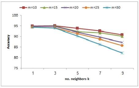
varied between 1 to 9 by step equals 2. Each point in the figures 5-6 represents the mean of 15 results with the same parameters. From Fig. 5 and 6, the classification accuracy slightly increases from k=1 to k=3 after that with the
increase of the value of k, the overall of classification
accuracy decreases. Furthermore, the higher the no. partitions m, the higher the decrease in the classification
accuracy with higher value of k. Hence, the difference
between the samples is significant and the classification accuracy will reduces. We can make a conclusion that k= 1
[image:4.595.36.263.501.649.2]of k may be set as small as possible since high value of k
means increase in runtime also. The value of k is extremely
[image:5.595.43.272.157.299.2]training-data dependent, changing the position of a few training data may lead to a significant loss of performance. Including the border objects of other partitions in addition to the the nearest partition increases the classification accuracy of the proposed method. Besides, it reduces the sensitivity of RC-RFkNN and LC-RFkNN for larger value of m and k.
Figure 5 Accuracy of RC-RFkNN for different values of nearest neighbors k and no. of partitions m on LETTER
The performance of the proposed methods for both k = 1
and k = 3 were high while for RC-kNN and LC-kNN the
[image:5.595.44.271.369.514.2]performance degrades for value of k higher than 1.
Figure 6 Accuracy of LC-RFkNN for different values of nearest neighbors k and no. of partitions m on LETTER
E. Performance Summary
In this experiment, in order to use the reported results in [17], the values of m and k are set to 10 and 1 respectively.
As shown in Table 4, we can observe that the proposed RC-RFkNN and LC-RC-RFkNN outperform RC-kNN and LC-kNN respectively. The amount of improvement increase as m
increases, as shown in Fig. 2-4 above. Also the proposed algorithm is less sensitive to the choice of k for small
number of k less than or equal 5 as shown in Fig. 5-6 . The
main advantage of the proposed algorithm is its stable
performance for high value of m compared to RC-kNN and
LC-kNN. As the number of partitions increases, the average size of NewX decreases resulting in a decrease in classification time with acceptable performance as shown in Fig. 2-6. Therefore, according to the experimental results, we may conclude that both RC-RFkNN and LC-RFkNN work well in terms of classification accuracy and time.
Table 4 Classification Accuracy of RFkNN compared to three algorithms on three datasets for m=10 and k=1
Dataset RC-kNN
LC-kNN
kNN LC-RFkNN
RC-RFkNN
LETTER 78.92 94.95 95.18 81.53 95.08 PENDIGIT 94.52 97.21 97.80 94.61 97.38 UPS 90.27 93.55 94.82 92.31 93.55
IV. CONCLUSION AND FEATURE WORK
Several existing efficient kNN classification algorithms are based on partitioning such as in [17]. This paper proposes an enhancement over these techniques by using the rough fuzzy set while conducting the clustering algorithm to separate the whole dataset into several parts. After clustering, each produced cluster is divided into two partitions: border and core. Only one core partition along with one or more border partitions are used in classifying unseen objects. The number of border partitions to be used depends on the unseen object's memberships in the clusters that are produced in the training phase. The proposed algorithm is a generalization of existing RC-kNN and LC-kNN algorithms [17]. Experimental studies are carried to select a suitable value for the input parameters for each dataset such as the number of clusters to be produced in the training phase m and the number of neighbors to be used in the
classification phase k. the traditional kNN is used as the base
line and several experiments are conducted on three standard datasets to compare the proposed RC-RFkNN and LC-RFkNN to the most related algorithms kNN, LC-kNN and RC-kNN. The experimental results showed that the proposed LC-RFkNN and RC-RFkNN outperform the corresponding techniques LC-kNN and RC-kNN respectively. The gain in performance in terms of accuracy with RC-RFkNN over RC-KNN was higher than LC-RFkNN over LC-kNN. The proposed approach inherits its efficiency from RC-KNN and LC-kNN since the added steps to both the training and testing phase are very simple. As a feature work, a new solution to perform an approximate k-nearest neighbors classification based on Spark may be developed to deal with big data [28]. We will also investigate the influence of using rough fuzzy set on the balance of accuracy and computation efficiency.
V. REFERENCES
[1] W.-J. Hwang and K.-W. Wen, "Fast kNN classification algorithm based on partial distance search," Electronics letters, vol. 34, pp. 2062-2063, 1998.
[2] Y. Song, J. Liang, J. Lu, and X. Zhao, "An efficient instance selection algorithm for k nearest neighbor regression," Neurocomputing, vol. 251, pp. 26-34, 2017.
[3] R. S. Michalski, J. G. Carbonell, and T. M. Mitchell, Machine learning: An artificial intelligence approach: Springer Science & Business Media, 2013.
Different Distances and Classification Rules," International Journal of Computer Applications, vol. 62, 2013.
[5] G. Bhattacharya, K. Ghosh, and A. S. Chowdhury, "An affinity-based new local distance function and similarity measure for kNN algorithm," Pattern Recognition Letters, vol. 33, pp. 356-363, 2012.
[6] M. J. Islam, Q. J. Wu, M. Ahmadi, and M. A. Sid-Ahmed, "Investigating the performance of naive-bayes classifiers and k-nearest neighbor classifiers," in Convergence Information Technology, 2007. International Conference on, 2007, pp. 1541-1546.
[7] T. İnkaya, S. Kayalıgil, and N. E. Özdemirel, "An adaptive neighbourhood construction algorithm based on density and connectivity," Pattern Recognition Letters, vol. 52, pp. 17-24, 2015.
[8] S. Zhang, X. Li, M. Zong, X. Zhu, and D. Cheng, "Learning k for knn classification," ACM Transactions on Intelligent Systems and Technology (TIST), vol. 8, p. 43, 2017. [9] I. Mani and I. Zhang, "kNN approach to unbalanced data
distributions: a case study involving information extraction," in Proceedings of workshop on learning from imbalanced datasets, 2003.
[10] V. Ganganwar, "An overview of classification algorithms for imbalanced datasets," International Journal of Emerging Technology and Advanced Engineering, vol. 2, pp. 42-47, 2012.
[11] M.-L. Hou, S.-L. Wang, X.-L. Li, and Y.-K. Lei, "Neighborhood rough set reduction-based gene selection and prioritization for gene expression profile analysis and molecular cancer classification," BioMed Research International, vol. 2010, 2010.
[12] O. Okun and H. Priisalu, "Dataset complexity in gene expression based cancer classification using ensembles of k-nearest neighbors," Artificial intelligence in medicine, vol. 45, pp. 151-162, 2009.
[13] S. D. Bay, "Nearest neighbor classification from multiple feature subsets," Intelligent data analysis, vol. 3, pp. 191-209, 1999.
[14] X. Wu, C. Zhang, and S. Zhang, "Efficient mining of both positive and negative association rules," ACM Transactions on Information Systems (TOIS), vol. 22, pp. 381-405, 2004. [15] X. Zhu, L. Zhang, and Z. Huang, "A sparse embedding and
least variance encoding approach to hashing," IEEE transactions on image processing, vol. 23, pp. 3737-3750, 2014.
[16] X. Zhu, S. Zhang, Z. Jin, Z. Zhang, and Z. Xu, "Missing value estimation for mixed-attribute data sets," IEEE Transactions on Knowledge and Data Engineering, vol. 23, pp. 110-121, 2011.
[17] Z. Deng, X. Zhu, D. Cheng, M. Zong, and S. Zhang, "Efficient kNN classification algorithm for big data," Neurocomputing, vol. 195, pp. 143-148, 2016.
[18] Z. Pawlak and R. Sets, "Theoretical aspects of reasoning about data," Kluwer, Netherlands, 1991.
[19] L. A. Zadeh, "Fuzzy sets," in Fuzzy Sets, Fuzzy Logic, And Fuzzy Systems: Selected Papers by Lotfi A Zadeh, ed: World Scientific, 1996, pp. 394-432.
[20] A. K. Jain and R. C. Dubes, "Algorithms for clustering data," 1988.
[21] R. J. Hathaway and J. C. Bezdek, "Extending fuzzy and probabilistic clustering to very large data sets," Computational Statistics & Data Analysis, vol. 51, pp. 215-234, 2006.
[22] S. Z. Selim and M. A. Ismail, "Soft clustering of multidimensional data: a semi-fuzzy approach," Pattern Recognition, vol. 17, pp. 559-568, 1984.
[23] M. A. Mahfouz and M. A. Ismail, "Efficient soft relational clustering based on randomized search applied to selection of bio-basis for amino acid sequence analysis," in Computer Engineering & Systems (ICCES), 2012 Seventh International Conference on, 2012, pp. 287-292.
[24] M. A. Mahfouz and M. A. Ismail, "Semi-possibilistic Biclustering Applied to Discrete and Continuous Data," in International Conference on Advanced Machine Learning Technologies and Applications, 2012, pp. 327-338.
[25] M. A. Mahfouz and M. A. Ismail, "Soft flexible overlapping biclustering utilizing hybrid search strategies," in International Conference on Advanced Machine Learning Technologies and Applications, 2012, pp. 315-326.
[26] "K. Bache,M.Lichman, UCIMach.Learn.Repos.(2013).", ed. [27] C.-C. Chang and C.-J. Lin, "LIBSVM: a library for support
vector machines," ACM transactions on intelligent systems and technology (TIST), vol. 2, p. 27, 2011.