Is consumption growth consistent with intertemporal optimization? evidence from the consumer expenditure survey

NUER WORKING PAPER SERIES

IS CONSUMPTION GROWTH CONSISTENT WITH INThRTEMPORAL OPTIMIZATION? EVIDENCE FROM THE

CONSUMER EXPENDITURE SURVEY

Orazio P. Attanasio Guglielmo Weber

Working Paper No. 4795

NATIONAL BUREAU OF ECONOMIC RESEARCH 1050 Massachusetts Avenue

Cambridge, MA 02138 July 1994

NBER Working Paper #4795 July 1994 ISCONSUMPTION GROWTH

CONSISTENT WITH INTERTEMPORAL OPTIMIZATION?EVIDENCEFROMTHE

CONSUMEREXPENDITURE SURVEY

ABSTRACt'

In this paper we showthat some ofthe predictions of models of consumer intertemporal optimization are not inconsistent with the patterns of non-durable expenditure observed in US household-level data, Our results and our approach are new in several respects.

First, we use the only US micro data set which has direct and complete information on household consumption. The microeconomic data sets used in most of the consumption literature so far contained either very limited information on consumption (like the PSID) or none at all, in which case consumption had to be obtained indirectly from income and changes in assets.

Second, we propose a flexible and novel specification of preferences which is easily estimable and allows a general treatment of multiple commodities. We show that a proper utatment of aggregation overcommodities can be important, both theoretically and in practice. Third, we present empirical results that show that it is possibletofind a reasonably simple specification of preferences, which controls for the effects of changes in demographics and labor supply behavior over the life cycle and which is not rejected by the available data. On our preferred specification, we obtain sharp estimates of key behavioral parameters (including the elasticity of intertemporal substitution) and no rejections of theoretical restrictions.

Our results contrast sharply with most of the previous evidence, which has typically been interpreted as rejection of the theory. We show that previous rejections can be explained by the simplifying assumptions made to derive empirically tractable equations. We also show that results obtained using food consumption or aggregate data can be extremely misleading.

Orazio P. Attanasio _{Guglielmo Weber}

Department of Economics Dipartimento di Scienzc Economiche

Stanford University UniversitA di Venezia

Stanford, CA 94305 Ca'Foscari

1. Introduction

In this paper we show that some of the predictions of models of consumer interteinporal optimization are not inconsistent with the patterns of non-durable expenditure observed in US household-level data. Our results and our approach are new in several respects.

First, we use the _only US micro data set which has direct and complete informationon

household consumption. Themicroeconomic datasets used in mostof the consumptionliterature sofar contained either very limited information on consumption (like the PSlD) or cone at all, in which case consumption had to be obtained indirectly from income and changes in assets.

Second, we propose a flexible and novel specification of preferences which is easily estimable and allows a general treatment of multiple commodities. We show that a proper treatment of aggregation over commodities can be important, both theoretically and in practice.

Third, we present empirical results that show that it is possible to find a reasonably simple specification of preferences, which controls for the effects of changes in demographics and labor supply behavior over the life cycle and which is not rejected by the available data.

Our results contrast sharply with most of the previous evidence, which has typically been interpreted as rejection of the theory. Several papers in the last 15 years have used microeconomic data to establish the plausibility of the intertemporal optimization model. Hall and Mishkin (1982), for instance, found that consumption is excessively sensitive to lagged labor income. Zeldes (1989) finds excess sensitivity for low wealth households and suggest that liquidity constraints arc important for these individuals. Results based on aggregate time series data, such as those in

Flavin (1981) and Campbell and Mankiw (1989), suggest even stronger rejections.

In this paper we interpret previous rejections as evidence against some simplifying assumptions made to derive empirically tractable equations. In particular, we show that:

a) aggregate data are particularly unsuitable to test the theory. Incorrect aggregation can lead to spurious rejections of the theory. Even in the simple case of isoelastic utility aggregation can be troublesome, as the theory requires knowledge of the logarithm of consumption. We use our household-level data to assess the consequences of neglecting the non-linearities implied by the model - andfind that theory restrictions can be rejected just because of an incorrect aggregation

procedure;

See also Carroll and Summers (1991) who observe that consumption tracks income over the life cycle. The papers by Runkle (1991), and Kane and Runkle (1992) are exceptions. Altonja and Siow (1987) appeal to measurement error to explain the rejections reported in some of the papers cited above.

b) food consumption, which is often taken as a 'proxy' for total non-durable consumption in studies using micro-data, 2is_{unsuitable because preferences are non-separable between food and}

other non-durables, and food is a necessity. Furthermore, during the sample period the relative price of food is far from constant. We show that the consequences of using food consumption rather than total non-durable_{consumption arenon-negligible: theory restrictions are rejected, and the} elasticity of intertemporal substitution is poorly determined when food is used.

We use a time series of cross-sections (the Consumer Expenditure Survey, 1980-90)_toconstruct consistently aggregated cohort-level data -a _{synthetic panel- where households are grouped by} year-of-birth and education. As discussed below, the availability of a relatively long time period is crucial in the estimation of Euler equations. Furthermore, thanks to the detailed information in the data set, we can construct different consumption_{measures, which include food and other} non-durable commodities.

The use of a micro economic data set which contains comprehensive information on consump-tion, income, leisure and household composiconsump-tion, allows us to address several questions directly. Our parametrization of preferences takes into account explicitly the possibility of non-homotheticity. The scheme we propose involves the estimation of a demand system, which allows us to construct the household-specific price indices that characterize the intertemporal allocation ofconsumption expenditure. In addition, we allow for the effects of demographic changes and leisure on intertem-poral allocation of expenditure. Finally, we can test theory restrictions in various ways, including

the popular excess-sensitivity tests.

-We_{show that a proper consideration of aggregation across commodities}

can be important for the estimation of key behavioral parameters. We also show that several simplifying assumptions commonly used in the literature, such as homotheticity and separability between_consumption and leisure are strongly rejected by the data. On our preferred specification, we obtain sharp estimates of key behavioral parameters (including the elasticity ofintertempora] substitution) and no rejections of theoretical restrictions.

The paper is organized as follows. Section 2 describes the data: it shows that income_and consumption age profiles track each other. This could be due to myopic behavior (as pointed out by Carroll and Summers, 1991), but could also be explained bychanges in demographics and leistire over the life cycle. In Section 2, we also show that both the relativeprice of food and its share in non-durable expenditure have varied considerably_{over the 1980s. Section 3 illustrates}

2 _An

same of the effects of incorrect aggregation across consumersandof using expenditure on food to describe intertemporal allocation ofconsumption. Section 4 describes in detail our specification of preferences which allows for non-homotheticity and non-separability between goods and leisure. Section 5 discusses econometric issues, with particular reference to problems which arise when the data are averages over relatively small sub-samples of the population. Section 6 presents estimation results: section 6.1 describes parameter estimates of a small demand system, which confirm the importance of non-homotheticity, and section 6.2 presents our estimates of the Euler equation. Section 7 concludes the paper.

2. Consumption behavior: data and descriptive analysis

Until recently, no micro dataset contained complete information on US household consump-tion. As stressed above1 most of the empirical work on the life-cycle model used the PSID, which contains only a measure of food consumption. Since 1980 the Bureau of Labor Statistics has been running the Consumer Expenditure (CEX) Survey on a continuous basis. The Survey is now available for 11 consecutive years which include two recessions and a long expansion, two major tax changes and witnessed substantial movements in relative wages and prices. The CEX is not a full panel (households are interviewed over four consecutive quarters, and then replaced); however, because it is available over a relatively long time period and it contains considerable demographic information, the use of synthetic cohort analysis allows the study of the evolution of consumption over the life cycle.

Therefore the CEX gives, for the first time, the possibility of analyzing individual consumption behavior over the life cycle and over the business cycle. In the next section we present a structural model for non-durable consumption which is not rejected by the data and allows us to estimate some key behavioral parameters. Before doing so, however, we describe the main features of the data used in estimation.

2.1 The GEl Survey

Thedata we use cover the period from 1980 to 1990. In this subsection we describe the data and the main selection criteria used. The CEX is based on a comprehensive survey run by the Bureau of Labor Statistics, which interviews about 4,800 households every quarter; 80 %ofthese

The unit of reference is what the BLS defines 'consumer unit' which consists of 'all members of a particular housing unit or other type of living quarters who are related by blood, marriage,

are then re-interviewed the following quarter, while the remaining 20 % are replaced by a new, random group. Therefore, each household is interviewed at moat four times over a period of a year. During the interviews, a number of questions are asked concerning household characteristics (demographics, work status, education, race, etc.) and detailed expenditures over the three months prior to the interview. The sample i5 representative of the US population.

We excludefrom our sample non-urban households, households residing in student housing, households with incomplete income responses. Furthermore, as discussed below, we consider only households headed by individuals born alter 1904andbefore 1965 and that are at least 19 and no more than 75 years old. These exclusion restrictions leave us with a sample of 146219 interviews. From each interview we consider, in addition to the demographic and labor supply variables die-cussed below, the expenditure figures for the month preceding the interview. The first two months of the quarter preceding the interview are excluded to avoid the fairly complicated error structure that the timing of the interviews would imply on quarterly data.

In what follows we consider various components of non-durable expenditure. In particular, for reasons to be discussed below, we look at food (defined as the sum of food at home, food away from home, alcohol and tobacco) and expenditure on other non-durable goods and services, such as services, heating fuel, public and private transport (including gasoline) and personal care, and semi-durables, defined as clothing and footwear. The major exclusions from total consumption expenditure are consumer durables, housing, health and education expenditure.

In the sequel we use two income variables: total after tax family income and total before tax 'labor' income. •Labor'_{income is defined as total family income minus capital income.} Unfortu-nately it is not possible to reconstruct the alter tax labor income.

In this paper we stress the importance of controlling for changes in the demographic structure of the household for a proper modelling of consumption behavior. We also stress the possibility that consumption and leisure might not be separable in the utility function. Therefore, even though it

Is Dot_{necessary to model labor supply explicitly, it is necessary to control for it. Fortunately, the}

adoption, or some other legal arrangement, such as foster children. Consumer unit determination for unrelated persons is based on financial independence. To be considered financially independent, at least two of the three major expense categories (food, housing, and other living expenses) have to be provided by the respondent'.

Such a complication would arise because there are households interviewed in each month and therefore their quarterly consumption would refer to overlapping periods.

Income data are collected at the first and last interview, and refer to the previous 12 months. Labor Income is also computed at second or third interview if a member of the household_reports changing her employment.

CEX contains a wealthofinformation on household characteristics and labor supply behavior. The demographic variables we examined in the empirical analysis are family size, number of children by age groups, number of adult members, number of persona older than 64, gender of household head, the educational attainment of the reference person, and the marital status of the household head.

The labor supply variables we have considered are various employment dummies, the number of earners, the number of hours worked by the wife and the dummies for part time and full time female employment.

The demand system in section 6 is estimated for different groups, formed on the basis of the educational attainment of the household head. The first group is that of high school dropouts, the second that of high school graduates, the third that of households with some college education and the fourth that of college graduates. Considering all years together the four groups account for 22.7, 29, 22 and 26.3 per cent of the total sample.

We devote a considerable amount of attention to the construction of appropriate price indices. Besides the parameters of the demand system discussed below, to construct such indices we need the price of the commodities we model (food and other non-durables). These are constructed from the components of the CPI published monthly by the Bureau for Labor Statistics. These prices are region-specific. The price indices for the composite commodities (food, other non-d urables) that form our demand system are then constructed as expenditure-share weighted averages of the elementary price indices. These prices are, therefore, household-specific.

To describe the intertemporal allocation of consumption we need also a nominal interest rate. We choose the return on Municipal Bonds as it is tax exempt, therefore avoiding us the difficulty of measuring individual marginal tax rates. We have also experimented with the 3-month treasury bill. Both interest rate series are taken from the Economic Report of (liePresident.

2.2 Life cycle and time series variation

In this subsection we describe the main features of the variables that are relevant for the more formal analysis of section 6. In particular, we characterize the life-cycle profile of non-durable consumption, household income, family composition and female labor supply. In addition, we examine the time series variability of prices and average consumption over the sample period under study. This analysis is useful not only as a descriptive tool, but also as an indirect check on the quality of the data set, which is relatively new.

The main _{problem with using}

the

CEX Survey for the analysisofa dynamic modelsuch as the life cycle one, is that each household is not observed over a long period of time. However, the continuity of the Survey allow us to follow the average consumption behavior of homogeneous groups over time, as they age. This is the main idea behind the synthetic cohort analysis which is used both in this section and in the more structural analysis in section 6.6

We divide the households in the sample in cohorts, defined on the basis of the year of birth of the household head.

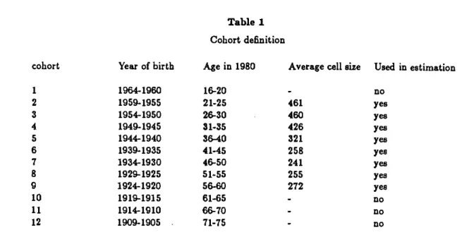
We then average the variables of interest over all the households belonging to a given cohort observed in a given year. If there are N cohorts observed for T years, this procedure gives use NT observations. In table 1 we report the cohort definition, their age in 1980 and the average cell size. The same cohort definitions are used in the section 5 to construct quarterly times series.

The advantage of grouping by the year of birth rather than by age in studying life cycle behavior is obvious. One follows over time a group of individuals born in the same period and therefore coming of age at the same_{time. Estimatingage profiles by pooling together several cross} sections and grouping by age is potentially very misleading in the presence of cohort effects.

In Figure 1 we plot average cohort log income and log non-durable consumption against age. Each connecting segment represents mean log income or consumption of a given cohort. Because cohorts are defined by a 5 year interval and the sample covers eleven years, each cohort overlaps with an adjacent cohort at 6 ages.

Both income and consumption are hump-shaped peaking before, retirement. Furthermore, consumption is considerably less variable than income: the standard deviation of the residuals obtained regressing first log consumption and then log income on a polynomial in age and cohort dummies is 0.04 and 0.06 respectively. This dJffereiice could be explained by smoothing behavior or by greater measurement error in income than in consumption.

The fact that b0th consumption and income present a pronounced hump (and the fact that differences in the shape of income profiles among occupation groups were reflected by similar differences in consumption profiles), is interpreted by Carroll and Summers (1991) as evidence against the life cycle model. Carroll and Summers, however, ignore family composition: in Figure 2, we plot the age profile of family size. As can be seen, the age profile for family size is also hump

• Details are given in section 5.

The household head is defined as the person who owns or signs the rental contract of the home where the consumer unit lives. For married couples, however,we define the husband as the household head and therefore use his age to establish to which cohort the household belongs to.

Table 1

Cohort definition

cohort Year of birth Age in 1980 Averagecell size Used in estimation

1964-1960 16-20

-

no

2 1959-1955 21-25 461 yes

3 1954-1950 26-30 460 _yea

4

1949-1945 31-35 426 _yea

5 1944-1940 36-40 321 _yea

6

1939-1935 41-45 258 _yes

7 1934-1930 46-50 241 _yea

8 1929-1925 51-55 255 yes

9 1924-1920 56-60 272 _yes

10 1919-1915 61-65 - no

11 1914-1910 66-70 - _no

Ii-

U-I

LA-

L2-C

0

Lfl 01 SW4W ra rta a@a

lb th

/

'I-

'OS-to —

S.,

-9—

a

log o stir In XuJisld li

/

/

40

1.2 —

S

M

a

—

.4 —

1500 —

Lcç o ft1y tte

th

I. £

1000 —

500 —

0—

2b

Figure 2

FsoI. arviual hiMs of ct

I

--20 40

shaped. '

In_{figure 3, we plot}the life-cycleprofile for female average annual hours of work. The average is conditional on the presence of the wife, but not on positive hours. Several features are worth noticing. First, female labor supply exhibits a substantial amount of variability both at life cycle and business cycle frequencies. Strong cohort effects are also apparent. Second, there i5 no apparent dip in female hours corresponding to fertility ages. This feature differentiates this profile from similar ones for other countries (like the UK) or other time periods.

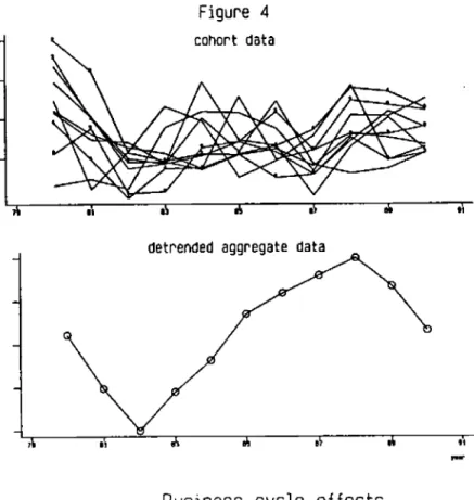
Several influences affect consumption and are partly detectable in Figure 1. We can think of life cycle effects, cohort effects and business cycle effects. In figure 4 we try to remove life cycle and cohort effects to isolate time effects. Of course this decomposition is somewhat artificial as the three kinds of effects are not identifiable. By regressing average cohort consumption on cohort dummies and a 5th degree age polynomial and considering the residuals of such a regression as time effects, we interpret all trends in consumption as deriving from a combination of cohort and age effects. In figure 4 these residuals are plotted together with de-trended aggregate non-durable consumption. Two features are noticeable. First, there is a substantial amount of synchronization across cohorts. The 1981-1982 recession is particularly visible. After that the average residuals seem to rise fairly steadily until the end of the sample. Second, average residuals follow reasonably well aggregate consumption. The correlation coefficient between the average residuals and aggregate de-trended consumption is around 0.4.

2.3Movements_{in consumption} shares andrelative_prices

In what follows, we give considerable emphasis to non-homotheticity and aggregation across comjnodities As Gorman (1959) has shown, the conditions under which one can aggregate across commodities and consider a single price index to characterize the allocation of consumption over time, are very stringent. If some goods are necessities and other goods are luxuries1 and their relative prices change, then at least two price indexes are needed to deflate nominal expenditure. Failing to model the features of preferences which prevent the consideration of a single price index introduces an omitted variable problem which can induce serious biases.

• There are also remarkable differences in the shape of family size acroes education and oc-cupation groups It is therefore possible that differences in consumption across education groups could be explained by differences in demographics. See the discussion in Attanaaio et al. (1994).

o The presence of measurement error and of definitional differences between CEX and national accounts consumption should also be kept in mind.

Figure 4

cohort data

Business cycle effects

'Ii

.09

.07

.05

.03

.01

—.01

Figure 5

.51

.49

.47

.45

-Figure 6

share of food

year

91

I I I I

In figure 5 we plotthe relative price offood and othernon-durablesover the 1980s. As can

be seen thereis a substantial amount of variability. In particular, around 1986 the relative price of foodand othernon-durablee exhibitsasubstantialshock. This is due to the decline in oil products priceswhich are included in non-durablee.

Correspondingto these changes in relative prices one can observe changes in consumption shares. In Figure 6 we plot the average share of food in non-durable expenditure over the 1980s. The graphs exhibit a substantial drop in 1982 followed by a more gentle decline up until 1985, when the share of food starts to increase again. Part of the dramatic drop of 1982 is probably explained by data problems. '° For this reason, in what follows, we report results for both the whole sample and a subsample which excludes the first two years.

In the first part of section 6 we modet the relationship between relative prices and food share when we estimate a simple demand system. Thisisthe first blockofour empirical strategy

to

modelnon-durable consumption expenditure. The necessity of such a step is evident in Figure 5.

3. What can we learn from aggregate data and from

food consumption?

As stressed in the introduction, most of the empirical work on the life cycle model of con-sumption has used either aggregate data or micro data which contained only limited information on consumption, namely expenditure on food. The use of the CES puts us in a vantage position, in

that we can replicate the results of other researchers and address the issues of aggregation across

consumers and commodities.

£1 Aggregation across consumers

Nobodywould doubt that actual consumers are heterogenous. Theissue, however, is to estab-lish to what extent heterogeneity affects inferences on the intertemporal optimization model based

on aggregate data. Attanasio and Weber (1993), using a long time series of UK cross-sections, have

shown that aggregation bias can explain the rejection of the overidentifying restrictions implied by

° The BLS runs a separate sample, based on diaries, rather than interviews, to collect infor-mation on expenditure on food and other frequently purchased items. In 1980 and 1981 (but not in later years) average food consumption was substantially higher in the interview survey than in the more reliable diary survey. A direct comparison with the share of food which can be computed from NIPA figures isnot feasible because of definitional differences in some of the items included in non-durable_{consumption. The}aggregate food share shows a constant and gentle decline which slows down around 1985.

the model. The Euler equation derived from isoelastic preferences implies a non-linear_relationship between consumption and the interest rate at the individual level. It iseasy to show that the use of aggregate data to estimate and test such a relationship is equivalent to taking the_{log of the} mean rather than the mean of the log. The difference between these two quantities is an index of inequality which, as shown by Attanasio and Weber (1993), has strong cyclical properties and therefore might cause the rejection of overidentifying restrictions." A similar exercisecan be per-formed using the CEX data. One of the advantages of working with a time series of cross-sections is that one can control the aggregation process directly: we can aggregate any known non-linear function of the individual data.

A tipical Euler equation derived from intertemporally separable and isoleastic preferences is the following:

(1)

_{Aiog(c',)= constanL+olog(l+rtti)+ct+i}

where ê is individual consumption, r is the real interest rate, a is the elasticity of intertemporal substitution and q is a residual uncorrelated with all the information available as of time t-l.

Equation (I) can be aggregated across consumers to obtain a similar equation for aggregated data.

(1')

_{jL09(4+z)=c0stant+o1og(1+rt+i)+ fE41}

In the absence of individual data researchers have estimated

(1")

_{tsiog, E(c'+i) =}

conatant_{+ clog(1 + r+1) + v÷1}

In table 2 we present estimates of equations (1') and (1"). We did not search for a satisfactory specification: the exercise is only meant to show the effects of incorrect aggregation.

The left-hand side column in table 2 reports estimates for the correctly aggregated non-durable consumption measure. The right-hand side column reports estimates for the incorrectly aggregated

"

The_{use of a representative consumer can be justified, theoretically, assuming the existence of} perfect insurance markets. Attanasio and Davis (1994) show overwhelming evidence against this hypothesis. Furthermore, even in the presence of complete markets, the non-linearity issue would still be relevant, unless we impose special preferences on the individual agents. In a recent paper, Mace (1991) reports results obtained using the CEX which could be interpreted in favor of the perfect insurance hypothesis. However, it is very easy to show that they could be caused by the presence of measurement error.

Table 2

Estimates basedon aggregate CEX data (weighted)

geometric arithmetic

mean mean

Aiog(favnsize) 0.942 0.668

(0.168) (0.207)

0.565 0.244

(0.230) (0.303)

Sargan Criterion 11.40 (11) 12.39 (11)

Breusch-Godfrey

Criterion 6.64 (4) 27.34 (4)

model (where we have taken the logarithm of the arithmetic mean, as is normally doneon aggregate time series data). 12 Four seasonal dummies (51-54)are_{introduced to take into account seasonality} in preferences. Changes in family size are also used as an explanatory variable. The real interest rate ii the final explanatory variable, and is treated as endogenous in estimation. We allow for an MA(1) error term reflecting measurement error and/or time aggregation1 by correcting all standard errors and choosing instruments lagged 2 or more quarters. 13

Two differences between the two columns are noticeable. First, the point estimates of the parameters are different. In particular, the coefficient on the interest rate, which is usually in-terpreted as the elasticity of intertemporai substitution, is less than half in size when estimated using incorrectly aggregated data. Second1 and more importantly, even though the Sargan test of overidentifying restrictions does not signal any violation for either equation, the Breusch- Godfrey test for correlation of second to fourth order strongly rejects the null for the equation estimated on incorrectly aggregated data. '

Higher order serial correlation is inconsistent with theory predictions, and would -_{given a} parsimonious instrument list -leadto the type of rejections of the overidentifying restrictions often reported in studies using aggregate data (e.g.: Hansen and Singleton, 1982).

As we argue in the following section, there are reasons to believe that equation (1') is mis-specified. The differences obtained estimating the two equations, however, are an indication of the importance of aggregation effects.

3.2 Food consumption

Most of the US literature on the life cycle model based on micro data has used the PSID, which contains only information on food consumption." This is a very serious limitation. The assumption necessary to justify the use of food to study the intertemporal allocation of consump-tion is that utility is separable between food and other consumpconsump-tion goods. All available studies of demand systems strongly reject such hypothesis. Furthermore, if the aim of the exercise is to estimate behavioral parameters, such as the elasticity of intertemporal substitution, it is

ques-12 We have used CEX-provided population weights to enhance _{comparability with published} National Accounts data, but similar results obtain when unweighted averages are taken instead.

13 The GMM estimator used to obtain the estimates in table 2 is the same as that used for the subsequent tables and is discussed in section & and in the appendix.

14 These results are similar to those reported for UK micro data in Attanasio and Weber (1993). Excess sensitivity tests fail to find a significant coefficient on income growth in either specification.

tionable whether those obtained using food consumption are indicative of the substitutability over time of total consumption. Finally, the isoelastic specification often assumed in empirical studies is particularlyill-suited for food,which is a necessity.

In Table 3, we_{reportthe results obtained estimating equation (1)}with consumptiondefined as expenditureonload. While the econometric technique used is slightly different," the_{specification} ofthe equationissimilar tothat estimated by several authors,such asZeldes_{(1989), Runkle(1991)}

andKeane and Runkle(1992). In column(1) the rate of growth in food consumption at the cohort level is related to the real interest rate (obtained subtracting the rate of growth in food prices from th nominal rate), and to other control variables such as seasonal dummies and the log of family size. Instruments used include second to the fourth lags of interest and inflation rates, second to the fourth lags of income, food and other non-durable consumption growth as well as a polynomial in age and lagged demographics. The results are not greatly affected by the introduction of other demographic variables or by a change in the instruments.

The estimate of the coefficient on the interest rate is negative and statistically different from zero. The Sargan criterion does Dot indicate a rejection of the overidentifying restrictions.

In the second column we add to the specification the rate of growth in labor income. The coefficient of this variable is estimated at 0.18 with a standard error of 0.07. Its introduction does not affect considerably the remaining coefficients or the test of overidentifying restrictions.

In the third column, we add to the specification in the second column the rate of growth of consumption of other non-durable commodities. The coefficient on this additional variable is estimated at 0.17 with a s.c. of 0.10, which makes it marginally different from zero. The point estimate of the coefficient on income is greatly reduced and it is no longer statistically different from zero. The coefficient on the interest rate is still negative and (marginAlly) different from zero. In the final column we remove the rate of growth of income. The coefficient on other non-durables is now strongly significant. The coefficient on the interest rate, however, is still negative, but not statistically different from zero.

We interpret the evidence in Table 3 as indicating that the non-separability between food and other non-durables is a potentially important problem.

The techniques used to obtain the results in table (3) are analogous to those used for the subsequent tables and are discussed in detail in section 5 and in the appendix.

As we pointed above, the food figures for 1980 and 1981 might be of particularly low quality. Because of this we re-estimated th columns in Table 3 over th, period 1982:3 to 1990:4. The results, available upon request, are very similar to those in Table 3.

Table 3

Estimates based on food consumption

(1) (2) (3) (4)

Alog 0.459 0.271 0.292 0.383

fam. size

(0.142) (0.165) (0.158) (0.160)

r

-0.733 -0.862 -0.551 -0.369

(0.253) (0.277) (0.363) (0.323)

tslog

-

0.177 0.101

laborincome - _{(0.067) (0.089)}

--

-

_{0.170 0.189}

othernon — durab. - - _{(0.104) (0.088)}

Sargan Crit. 12.1 11.6 10.2 10.2

p-value (0.88) (0.86) (0.89) (0.95)

Number of 288 288 288 288

observations

The estimates of the elasticity of food consumption growth to the real interest rate presented here differ from those available in the literature. " These differences could be due to a variety of factors including,for instance,the use of a different survey in which the timing of food expenditure

is better determined. An important difference is in the econometric methodology. The use of syntheticpanels(rather than a short panel at the individual level) affords important gains in the time dimension of the sample. Given that the error term has an expectational component, this is a matter of great importance (consistency issues are further discussed in section 5).

4. The allocation of consumer expenditure over time with multiple commodities

Food is a necessity and it is unlikely, as we have shown in the previous section, to be separable from other non-durables. Therefore food expenditure is inadequate to study the intertemporal allocation of consumption. On the other hand, even when data on total non-durable expenditure are available, it is not obvious that its intertemporal allocation could be described, in the presence of large changes in relative prices, by a single price index. It might be necessary to model the intratemporal and the intertemporal allocation of consumption simultaneously.

In this respect several modelling strategies are available. One could formulate within period utility as a function of several commodities and consider the Euler equation for each of them. The main problem here is to find a flexible direct utility function which nests the isoelastic case (and for which integrability conditions can be imposed by setting data independent restrictions on the parameter space). Alternatively, one could consider flexible specifications for marginal utilities and estimate the Euler equations from those. In this case, however, quasi- concavity of the implied utility function might be hard to impose. Finally, one can choose to work with an indirect utility function which captures both non-homotheticity and non-separability.

We adopt this last strategy. While most of the theoretical results used in the analysis are well known at least since Gorrnan (1959), the specification of preferences we present is relatively new. We introduce an empirically tractable way to consider the intertemporal allocation problem when within period utility depends on several commodities. Our specification relaxes the assumption of homotheticity and therefore does not allow the characterization of intertemporal allocation by means of a single price index. The homothetic case, however, is nested as a special case and can be obtained with simple restrictions on the parameters we estimate.

Our specification of preferences is similar to that used by Blundell, Browning and Meghir

"

_{See,for instance, Zeldes (1989), Runkle (1991), Keane and Runkle (1992).}

(1994) in a recent paper, but presents the key advantage of pkoducing an Euler equation for consumption which nests equation (I) when preferences are homothetic.

We proceed in two steps. We first estimate a flexible demand system which satisfies integra-bility conditions. The results obtained in this first step are then used to construct the, price indexes necessary to characterize intertemporal allocation. The parameters that enter the Euler equation can then be estimated.

4.1 Multiple Commodities and the Euler Equation

Let_{us first consider the representative agent problem as formulated in most macro economic} papers:

(2a) Max

(2b) suhjcct to A÷1 = (1 + r.1)A + v —pc4

where A are the assets at the beginning of period 1, c is expenditure on an homogeneous and non-durable consumption good, y is income in period t, and r,.1 is the nominal interest rate between periods t and t + 1.

Equations (2a) and (2b) give rise to the standard Euler equation for consumption. In the literature, the instantaneous utility function is often parametrized as the following CRRA utility function which gives constant elasticity of intertemporal substitution equal to a.

(2c)

U(c)=

Equation (1) in the previous section can be obtained log-linearizing the first order condition for the maximization problem (2a)-(2c).'° When one considers several commodities, one can think of as total expenditure deflated by an appropriate price index. However, as Gorman (1959) proved,

"

_{Theconstant of equation (1) includes the log of the discount rate ftandvarious terms reflecting}

second and higher moments of the conditional distribution of c1.,. If 's+iis_{conditionally} log-normal, the constant will include only the variances of consumption growth and the interest rate as well as their covariance. An implicit assumption which is usually made is that changes in these conditional moments are uncorrelated with the instruments used.

only under very stringent conditions the intertemporal optimization problem can be determined on the basis of a single price index.

One can interpret (2a) as the utility index of a consumer who breaks her optimization problems in two steps: in the first step, she decides how much total expenditure X to allocate to each time period. In the second step, she allocates X to different goods (q1 ,_{... ,qN), according}to their relative prices and to X itself (some goods will be luxuries, some necessities). Suppose the second step produces demand equations of the Almost Ideal type (see Deaton and Mueilbauer (1980)):

(3)

a +y,1n(p,s) +fl1[in(X,)

— Ina(pg)]

where_{the p's are individual prices (and p is the corresponding price vector), and a, i and fl's are} preference parameters (which will be functions of demographic characteristics, employment, etc., as in Blundell, Pashardes and Weber (1993)). If all the fl's are zero, preferences are homothetic, and the indirect utility function for period-t consumption is:

(4) V =

= F[c]

where Ff4 is a monotonic transformation (which cannot be identified from the demand sys-tem alone and determines the intersys-temporal allocation), and tn(a(pg))

= a

+ Eadn(pi,) +

.5 1

• %,tn(p1jln(p11). Equation (4) implicitly defines c as nominal expenditure Kg deflated

bya(p,).

On the other hand, if the fl's are non-zero, violating homotheticity, the indirect utility function becomes:

(5)

V =

F[(-9i*t

where b(p,) =

_fl,p

_,i.e_{a zero-degree homogeneous price index (adding-up implies Eflj = 0).This} second price index takes into account the different impact price changes have on utility according to the type of good they refer to (ft, >0_{for luxury goods, fl cO for necessities).}

Neglecting the existence of this second price index may lead to spurious inferences. Equation (1) will suffer from omitted variable bias, because no account is taken of changes in h(p,) over time. This problem is particularly severe if, over the sample period analyzed there are large

chnges in relative prices across luxuries and necessities (for instance, if luxuries become relatively more expensive in booms, and cheaper during recessions).

If we substitute equation (2a) with the following,

(6)

U=>j-_r[(fj)r ]'-t(i+5)-'

theEuler equation (1) becomes:

(7)

+ c(b(pi) —

= ' +

e[r.1

— aJn(b(p,1)J

+

Thisexpression looks daunting, but neatly simplifies to equation (1) when all the fl's are zero (in which case b(p) =_1). 20

Whenthe fl's are not zero, the second price index is subtracted from the standard definition of the real interest rate, and it affects the coefficient on consumption growth. The equation is easy to estimate, particularly if the fl's are known in advance: this is the case if we estimate Engel curves separately in each year. However, a is no longer the elasticity of intertemporal substitution: its multi-good definition is (Browning, (1987)) MS = _{(—) fr— where}an x subscript denotes the partial derivative with respect to X. This implies:

MS ——— ab(p)

l+o(b(p)—i)

We can rewrite equation (7) as

(7')

In(c,+1) = '+ ofr.,. — &n(6(p,,1) —

A(In(c,+s) — in(ct+z) b(p11)

3° Blundell,Browning and Meghir (1994) estimate an Euler equation similar to (7), but with further non-linearities. Their analysis is different in two respects. On the one hand, their demand system is more general than ours as it is consistent with a wider pattern of Engel curves (and nests the Almost Ideal case from which we start). On the other hand, their monotonic transformation in V takes as argument a non-linear function in X. This second feature implies that even in the homothetic case their Euler equation does not simplify to equation (1). In the Almost Ideal case, for instance, their Euler equation involves taking the logarithm of log(consumption) -a_particularly

unappealing data transformation, which rules out very low, but theory-consistent consumption levels.

which is the specification we use in our empirical work. Herç- the dependent variable is the first difference in the log real consumption divided by b(p) (a number close to 1). On the right-hand side, the real interest rate (obtained subtracting from the nominal rate the rate of inflation in a(p)) is_{further deflated by the growth rate of the second price index, b(p),and by a correction}

term, which is the difference between consumption growth as normally defined and the dependent variable.

4.2 Thning up themodel

Before even trying to fit the model described above to• the data, a number of simple mod-ifications are necessary. These allow the model to explain some obvious, and yet quantitatively important, features of the data.

(1) Household consumption exhibits large seasonal fluctuations which are clearly inconsistent with a simple minded version of the life-cycle model. A simple way of introducing seasonal fluc-tuations is to have the utility function depending on seasonal shifts, so that a given amount of expenditure gives different levels of utility in different quarters. This framework has been used (among others) by Miron (1986) on aggregate data and by Attanasio and Weber (1993) on micro data. In the log-linearized Euler equation used in this_{paper1 this specification implies the use of} seasonal intercepts in a regression of the rate of growth of consumption on the interest rate.

(ii) The utility derived from a given amount of expenditure obviously depends, among other things, on family composition. In general, it is quite difficult to model properly intra-household decisions. Fertility choices are probably endogenous and should be modeled simultaneously with consumption and labor supply behavior. However, it is quite easy to introduce some simple cor-rections to make the model more realistic. We assume that utility is shifted by a number of demographic variables such as the number of children of various ages, the number of adults, etc. Such a framework allows for fairly flexible adult equivalent schemes. The instantaneous_utility function for a generic household It that will be used in the empirical application below is the following:

=

_{U(C')qS(Z11',9)}

where C is total family expenditure and _,9)is a function of various demographic variables. If the function 0 is given by O(Zt,9)

= ezp(9'Z),

the term 9SZ1' will enter the Euler equation for consumption. Changes in _{are equivalent to a time-varying discount 6. For this reason we}

shalt refer to 4'as'the discount factor'.

Demographic variables are also likely to affect the demand system. As a consequence they will, also have an indirect effect on the Euler equation through the price indexes a(p) and b(p).

(iii) An implicit and potentially controversial assumption often used in papers that estimate Euler equations for consumption is that of separability of the utility function between consumption and leisure. While in this paper we do not model explicitly labor supply behavior, we argue that non-separability between consumption and leisure can be taken into account in a very simple way. Common sense tells us that the level of utility obtained from a given amount of expenditure depends on labor force participation variables: when a member of the household works, he or she will have to bear a number of job-related expenses that will be reflected in total consumption expenditure. These job-related expenses will affect both the intertemporal allocation of expenditure (normally increasing expenditure when leisure is low) and the intratemporal allocation (by making leisure-intensive commodities relatively more expensive). For this reason, we allow for leisure effects in the demand system -thusproducing price deflators that depend on leisure, but also capture direct intertemporal leisure effects by introducing leisure-related variables in the Euler equation.

In practice, we introduced as determinants of the marginal utility of consumption a number of labor supply variables, reflecting both employment status and hours. This strategy allows us to avoid the formal modeling of labor supply, with the complications arising from corner solutions and institutional constraints. This obviously only identifies conditional preferences (see Browning and Meghir (1991)).

5. Econometric Issues

As we said in Section 2, the CEX survey is a rotating panel. Rather than employing the (short) panel dimension of the survey, which is probably dominated by seasonal factors, we decided to construct synthetic panels. We define cohort by the year of birth of the household head. Our technique is equivalent to using the interaction of time and group dummies as instruments. We impose an age limit (23-60) and a cell size limit (150) on the cohorts we consider, so that our synthetic panel is not balanced. 22

21 An _{analogous parametrization applies to the non-homothetic case, where C is defined as}

(.

'(Ri)

See Deaton (1985), Browning, Deaton and Irish (1985) and Moffitt (1993). We also experi-mented with groups formed by year of birth and educational attainment. The education groups were the same as those used in the estimation of the demand system. The reason we only report

There are several advantages in the use of synthetic panel techniques to estimate an Euler equation. First, averaging over individuals belonging to a group should eliminate additive idiosyn-cratic measurement error.

Second, it is known that if the panel dimension is short, the introduction of household specific fixed effects gives inconsistent estimates, unless the instrument used are strictly exogenous (see Runkle (1991)). Taking cohort averages over long time periods can get round this problem: because we observe groups for the whole sample period (at least potentially), the relevant dimension is the total length of the period covered by the survey, not how long each household stays in it. A similar argument can be made about the presence of aggregate shocks. If we think our sample is long enough so that expectations! errors are averaged out, the use of more or less standard IV techniques gives us consistent estimates. This solves the small T problem discussed by Chamberlain (1984) and Hayashi (1987).

Third; we do not need to worry about attrition as much as we should if we were using a long panel. In this respect, as stressed by Moffitt(1993), the use of a time series of cross section has some advantages relative to the use of panel data.

Fourth, even though we work with aggregate data, in that we sum over the individuals be-longing to a certain group, we can control the aggregation process directly. In this respect, as we saw in section 3, we can perform interesting exercises to evaluate the extent of aggregation biases. The use of synthetic panels, however, does not by itself solve some important econometric problems. First, it does not help deal with non-additive measurement error. We should stress that any form of non-additive measurement error in the variables of which we take averages, induces inconsistent estimates. Second, it does not eliminate concerns about non-random attrition. In particular, we have to rely on the assumption that the population from which the sample is drawn is homogeneous over time. This assumption might be violated if, for instance, there is a relationship between mortality and wealth. If this is the case each cohort would become progressively 'richer' as it ages and therefore we would overestimate the rate of growth of consumption for older cohorts. Averaging over cells of relatively small size induces measurement error in the levels, which

results based on birth year cohorts is that by crossing cohorts and education groups we are left with very small cells giving rise to extremely noisy data. The results were extremely imprecise.

_"

Of course this argument impinges on the assumption that our sample is large enough so that expectational errors are averaged out. While 44 quarterly observations might not be a very large

number, it should be stressed that our sample period includes two recessions and a long period of

moderate growth.

in turn implies an MA(1) structure in the first differences. 24 The reason for this is obvious.

if

the sample for a given quarter t includes a very rich household, this will induce a positive measurement error in the consumption growth at tune t followed by a negative measurement error a time t+ 1. The error of equation (1) is therefore going to be made of two components. A white noise component which reflects expectational errors and an MA(l) component with a coefficient of -1. The sum of a white noise and an MA(1) is an MA(l). The size of the coefficient of this MA(l) depends on the relative magnitude of the variances of the expectational error and of the measurement error.

if the only error to equation (1) and its extensions was an expectational one, instruments

dated t

— I _{and earlier would be valid ones. Our data, however, do indicate negative first order}

autocorrelation, thus suggesting that measurement error is an important issue. Because of this, the instruments dated t— I _{are invalid, but instruments lagged 2 and more periods yield consistent} estimates.

The panel dimension of the CEX implies that temporally adjacent cells do not include com-pletely different households. For instance, households at their first interview in time period t,

appear

also at time + 1, t

+ 2 and

t

+ 3. On the other hand those at the 4th and last interview

at time t, alsoappear at time t— 1, —_{2 and t— 3. If we ignore the rotating nature of the panel}

and use all the households in the construction of the relevant variables and of the instruments, we get inconsistent estimates in the presence of household specific fixed effects. On the other hand, using only one interview per household involves the loss of a substantial amount of information.

To get around this problem we use all observations in the construction of the variables that enter our regression and select subsamples on the basis of the interview number in the construction of instruments. Namely, we use only households at the fourth interview in the construction of lag 2 instruments, households at the fourth and third interview for lag 3 instruments and we exclude households at the first interview for lag 4 instruments. This scheme guarantees that there is no overlap between the households used in the construction of the instruments and those used in the construction of the variables that enter the estimated equation.

24 _{Thepresence of measurement error induced by small cell size is relevant for all the}

household-specific variables considered in the equation, even for those, such as family composition, that could be conceivably be considered as exogenous. The only exception is age, that we define as median cohort age, and is therefore unaffected by sampling variability.

Hall (1988) suggests that if the planning horizon is shorter than the frequency of the observed data, the Euler equation has MA(l) errors. The sum of two independent MA(1) processes is again an MA(1)process.

The presence of MA( 1) residuals for each cohort is not the only problem with the error struc-ture of equation_(1). Because we estimate it for N cohorts simultaneously, the expectational errors for a given time period for different cohorts are likely to be correlated. We allow for contempo-raneous correlation among the residuals of different cohorts. We also allow for the presence of arbitrary heteroscedasticity which is likely to arise because of differences in cell sizes.

The complicated error structure of equation (1) estimated for several cohorts simultaneously has to be taken into account in the construction of an efficient estimator and in the estimation of its standard errors. 26 Detailsare provided in the appendix, where we describe in detail the GMM estimator we use.

A final issue is the way we treat instruments. In principle, we could 'stack' the instruments for each cohort (effectively imposing the same reduced form for all cohorts), or we could have different first stage regressions for each cohort. Given the limited number of obsenations, we decided to 'stack' the instruments.37

6. Results.

This section describes the results obtained estimating our preferred specification. First, we present the estimation of a simple demand system. This shows that the we need at least two price indexes to describe intertemporal allocation over time. This follows from the fact that food consumption is a necessity and fromthe fact that over the sample period the relative price of food and other non-durable changed dramatically.

The estimation of the demand system allows us to construct the price indexes which are necessary to determine intertemporal allocation. We show the time series behavior of these price indexes and discuss the implications of their omission.

Second, we present the results obtained estimating equation (7') and contrast them to those obtained estimating equation (1).

5.1 Demand system

26 A_{GLS type transformation can generate inconsistent estimates if involves filtering the system}

backward (see }layashi and Suns (1983)). Deaton (1955) shows that the cross sectional second moments can be used to improve the efficiency of the standard Instrumental Variable estimator, by giving less weight to the instruments more affected by sectional variability. Unfortunately, as noted by Fuller (1987), there is no guarantee that the resuJting projection matrix be positive definite in finite samples. We do not make use of these corrections because of their finite sample unreliability.

We split total non-durableexpenditure on food and all other_{non-durable goodsand services.} This split, while arbitrary, has the advantage of grouping (potential) necessities separately from (potentiai) luxuries, and of defining commodities for which zero expenditures are notreported.

The two-commodity demand system we estimate is of the Almost Ideal

type (see equation (3) above): the dependent variables are the budget shares of food and of other non-durables, the explanatory variables are their prices and total non-durable expenditure (the budget), deflated

by a linearly homogenous price index, a(p). Because the budget shares add_{up to one an equation is} redundant and we estimate and report just the food equation without loss of_generality.

In principle, all preference parameters (a, and_fl's)could_{vary across households. We restrict}

their variation in the following ways: we assume 7's and ft's to be constant within_educational groups, and the a's to depend on a few demographic and labor market variables. We therefore estimate separate budget share equations for food for each of four groups formed on the basis of the education attainment of the household head: high school dropouts,_{high school graduates,} college dropouts and college graduates. For each educational group the a parameter (which affects both the intercept and the a(p) index deflating nominal expenditure) is allowedto depend on some deterministic variables (seasonal dummies and a zero-one indicator for the 1980-1 wave of interviews), some demographic indicators (age of the head, single adult dummy, total number of family members, number of children) and a few zero-one labour market variables (head_unemployed, second adults works full time, second adult works part time, log of female leisure). Al! of these variables affect significantly the budget share of food for at least one educational group, but none of the non-deterministic variables plays a key role in determining the ft_{parameter,i.e. the degree} on non-homotheticity.

In order to avoid the measurement error problems (discussed in Blundell, Pashardes and Weber, 1993) which plague household- level data, we have estimated consistently aggregated budget share equations at the cohort level. This i5 equivalent to treating all explanatory variables as endogenous, and using year-quarter-cohort dummies as instruments. We concentrated on 10year-of-birth cohorts and therefore have 430 observations for each equation. In estimationwe impose all theory restrictions (homogeneity is never rejected;_{symmetry is marginally rejected in two of} the four equations).

In Table 4, we report parameter estimates for ftand_{descriptive statistics of some key}

elas-ticities by educational group. Two things are worth noticing. Fiat, the estimatesconfirm, not surprisingly, that food is a necessity. Second, the budget elasticities of food expenditure decline

Table 4

Elasticities derived from the daniad syBtem

budget elasticity uncoinpensated price

(s.e) at the mean elast. at the mean

High School dropouts -.064 0.877 -.577

(.016) (0.03) (0.06)

High School Graduates -.074 0.841 -.513

(.016) (0.035) (0.06)

College Dropouts -.099 0.781 -.580

(.011) (0.025) (0.06)

College Graduates -.166 0.616 -.438

(.011) (0.027) (0.08)

inonotonically with educational attainment, ranging from 0.88 for high school dropouts to 0.61 for collegegraduates. Price elasticity is lowest for college graduates and (in absolute value) consider-ablyless than unity.

6.2Euler equations

In Table 5, we report the results obtained estimating the Euler equation (7). They incorporate the estimates of the demand system discussed above through the price indexes and_{are obtained} by the 0MM techniques discussed in section 5 applied to average cohort data. 25

In the first 3, columns we present estimates of three different specifications for the entire sample period and 8 cohorts. Because, as stressed above, the 1980 and 1981 survey might be of lower quality we re-estimate the three specihcations on a shorter sample period. We_{report these} results in columns 4 to 6.

To the basic specification (7'), we add several variables which are meant tocapture the effects of changing family composition and labor supply on the discount factor #0. Aftertrying several specifications we settled on the one reported. The main conclusions we draw are robust to the inclusion of additional demographic variables or to the exclusion of some of the less_significant ones.

In the specification reported the discount factor #(.)is_{assumed to depend on seasonal} durn-mies, on the log of family size, on the number of children between the ages of 0 and 15, on a dummy which equals unity if the wife works full time, on the log of annual hours of leisure enjoyed by the wife (computed as 5000 minus the number of hours of work) and a dummy for single individuals. Other variables that were considered during the specification search include the number of chil-dren of various ages, a dummy for part time working wife, and the number of earners. 29 We also considered variables such as the number of vehicles and dummies for home-ownership.

All variables in the equation, with the exception of seasonals, are instrumented. There sic two reasons to use this procedure. First, some of the variables considered are choice variables determined simultaneously with consumption. Second, all of them are subject, given the size of our sample1 to measurement error. As argued above the_{presence of measurement error and} therefore of MA(l) residuals makes lag-one instrument invalid. The instruments used were second,

25 No attempt is made to correct the standard_{errors for the use of generated regressors.} The cohort average of a dummy variable (such as that for working wifes) measure the propor-tion of households, within a particular quarter- cohort cell, which satisfy a particular condipropor-tion.

Table 5

Euler equation for total consumption expenditure

Using resultS from the demand system

(1) (2) (3) (4) (5) (6)

0.559 0.421 0.271 0.668 0.589 0.424

0.43 _{(0.224) (0.250) (0.189) (0.189) (0.201) (0.156)}

Alfmsz

1.351 1.213

-

1.619 1.563

-0.17 (0.357) (0.375) - (0.340) (0.356)

-achildren -0.498 -0.451 - -0.487 -0.431

-0.18 _{(0.156) (0.167)}

-(0.155) (0.163)

-Aww -0.816 -0.857 - _{-1.469 -0.924}

-0.12 _{(0.442) (0.435)}

-(0.967) (0.462)

-&nwl

-1.437 -1.222 - _{-0.696 -1.314}

-0.09 _{(0.835) (0.797)}

-(0.751) (0.902)

-Ssingle -1.214 -1.038

-

-1.211 -1.712

-0.12 _{(0.712) (0.683)}

-

_{(0.828) (0.773)}

-Alt,

-

0.121 0.306 0.107 0.090 0.247

0.25

.

_{(0.090) (0.068) (0.155) (0.068) (0.048)}

Sargan crit. 17.18 18.29 25.70 18.40 19.31 30.29

(p-value) (0.64) (0.50) (0.36) (0.56) (0.44) (0.18)

Eat, period 81:3-90:4 _81:3-90:4 81:8-90:4 82:3-90:4 82:3-90:4 82:3-90:4

Cohorts 1-8 1-8 1-8 1-8 1-8 1-8

Ol,s. 288 288 288 256 256 256

Notes: _{Asymptotic standard errors}in parentheses. All specification. includea constant a

three seasonaldummies. The instruments set is the same across columns and includes the second to_{fourth lag of consumption growth, inflation,} nominal interest rates andlabor income _growth, the second an third lag of all the other variables incolumn (1), thesecond and third_{lag of the} number_{ofearners, three seasonal dummies, age, agesquared}and a constant. The numbersunder the variable names are W of the first step regression onthe 81:3-90:4 sample.

Legend:

r

=

real interest rate,If rnsz=log offamily size, tow

=

dummyfor wife working

full

time,

lnwl =

log ofwife'sannual hours _{of leisure,single=dummyforsingle consumers, ly =log}

third and fourth lag of interest rates, consumption and income

growth and inflation, the second and third lag of all the variables considered in the discount factor, nad of the number of earners,_age, age squared1 a constant and three seasonal dummies. The reasons behind this choice of_instruments are discussed below.

In the column with the variable names we report the R21s of

the first step regression of each of the variables on the instruments (for the longer

sample). In colwnns (1) and (4) we

report our favourite specification. The coefficient on the interest rate is related_{to the elasticity of} intertemporal substitution (cia) as evident from equation 7'. When preferences are homothetic so that 6(p) =_1,

such a coefficient is actually equal to the cia. In practice, theestimated parameters of our demand system and the behavior of relative prices, imply a

very small variability of b(p) which, in the sample, ranges from 0.99 to 1.01. Therefore, for allpractica] purposes, we can consider the estimated coefficients on the real interest rate as an estimate of the cia. This coefficient is estimated at 0.56 (s.e.= 0.22) for the whole sample and at 0.67 (s.e.

=

_{0.19) for the shorter period. This} relatively high estimate of the cia is consistent with the result reported for the UK in Attanaaio and Weber (1993).

As is evident from the estimates, some of the demographic variables are quite important. Attanasio et al. (1994) plot the life cycle profiles for the discount factors implied by a specification similar to the present one and estimated on the same data set. They show that, when used to solve and simulate a life cycle model, these estimated discountfactors are able to generate not only the hump shaped profile which characterizes life cycleconsumption, but also the differences across education groups, SO

In

columns (2) and (5), we add to the specification in columns(1) and (4), the rate of growth

in labor income (including transfers). '

_The

finding of a non-zero coefficient on this variable has been interpreted in the literature as evidence of_{excess sensitivity of consumption to labor} income. The coefficient we estimate is relatively small and is_{not significantly different from zero.} This result cannot be explained with the fact that the instruments used are unable to capture the variability in income growth: the R' of the first step regression for income_{growth is approximately} 0.25, which is higher than the R2 for all the demographic and labor_{supply variables. Indeed, the} main motivation for the inclusion of so_{many instruments and in particular of the lagged values}

°

_Even

though the taste parameters are assumed to be the same_{across education groups, the} discount factors (and therefore the implied_{consumption profiles) will differ because the forcing} variables -_demographics

and labor supply- will differ across education groups. We also tried the rate of growth in total after tax

Table 6

Euler equaflon for total consumption expenditure

Using Stone price index to deflate total non-durable expenditure

(1) (2) (3) (4) (5) (6)

0.341 0.149 0.221 0.480 0.331 0.442

(0.276) (0.347) (0.263) (0.282) (0.316) (0.218)

Alfmsz

1.172 0.948

-

1.539 1.413

-(0.399) (0.479)

-

(0.383) (0.417)

-Achildren -0.539 -0.453

-

-0.617 -0.558

-(0.169) (0.200)

-

(0.186) (0.192)

-ww

-1.551 -1.560

-

-1.808 -1.826

-(0.666) (0.639)

-

(0.665) (0.649)

-AInwl -2.578 -2.486

-

-3.207 -3.011

-(0.835) (1.046)

-

(1.185) (1.144)

-4.81n91C -2.239 -2.157

-

-2.744 -2.567

-(0.912) (0.906)

-

(0.828) (0.987)

-- _{0.100 0.268}

-

0.094 0.223

- _{(0.103) (0.067)}

-

_{(0.089) (0.053)}

Sargan crit. 11.66 12.34 23.32 12.11 13.06 25.99

(p-value) (0.92) (0.87) (0.50) (0.91) (0.84) (0.35)

Eat. period 81:3-90:4 81:3-90:4 81:3-90:4 82:3-90:4 82:3-90:4 82:3-90:4

Cohorts 1-8 1-8 1-8 1-8 1-8 1-8