Distributing test cases more evenly in adaptive random testing

(1)

Distributing Test Cases More Evenly in

Adaptive Random Testing

∗

Tsong Yueh Chen, Fei-Ching Kuo, Huai Liu

†

Faculty of Information and Communication Technologies

Swinburne University of Technology

John Street, Hawthorn, Victoria 3122, Australia.

Abstract

Adaptive Random Testing (ART) has recently been proposed to

enhance the failure-detection capability of Random Testing. In ART,

test cases are not only randomly generated, but also evenly spread over

the input domain. Various ART algorithms have been developed to

evenly spread test cases in different ways. Previous studies have shown

that some ART algorithms prefer to select test cases from the edge part

of the input domain rather than from the centre part, that is, inputs

do not have equal chance to be selected as test cases. Since we do not

know where the failure-causing inputs are prior to testing, it is not

desirable for inputs to have different chances of being selected as test

cases. Therefore, in this paper, we investigate how to enhance some

∗_{A preliminary version of this paper was presented at the 18th Australian Software}

Engineering Conference (ASWEC 2007) (Chen et al., 2007b).

†_{Corresponding author. Tel.: +61 3 9214 5276; fax: +61 3 9819 0823.}

(2)

ART algorithms by offsetting the edge preference, and propose a new

family of ART algorithms. A series of simulations have been conducted

and it is shown that these new algorithms not only select test cases

more evenly, but also have better failure detection capabilities.

Keywords: Software Quality, Software Testing, Random Testing,

Adaptive Random Testing, Test Case Distribution.

1 Introduction

Software testing is a major approach to software quality assurance. There

exist many testing methods which actively select inputs for testing (namely

test cases) in order to effectively detect software failures. Random

Test-ing (RT) is a basic software testing method, which simply selects test cases

in a random manner from the set of all possible inputs (namely the input

domain) (Hamlet, 2002; Myers, 2004). RT has many advantages as a

soft-ware testing method. For example, it can automatically generate a large

number of test cases at low cost, and the test case generation is not

influ-enced by any human bias. What is more, its “randomness” may help reveal

failures which cannot be detected by deterministic approaches (such as

do-main testing (White and Cohen, 1980), data flow testing (Laski and Korel,

1983), and branch testing (Myers, 2004)). Because of these advantages, RT

has been successfully applied to detect software failures in industry, such as

the testing of UNIX utilities (Miller et al., 1990, 1995), SQL database

sys-tems (Slutz, 1998), Windows NT applications (Forrester and Miller, 2000),

Java Just-In-Time compilers (Yoshikawa et al., 2003), and embedded

soft-ware systems (Regehr, 2005). However, some researchers (Myers, 2004)

ar-gued that RT may be the “least effective” testing method because it uses

(3)

A number of studies (Ammann and Knight, 1988; Finelli, 1991; Bishop,

1993) have independently shown a common characteristic about most faulty

programs, that is, program inputs that can reveal failures (namely

failure-causing inputs) tend to cluster together. Ammann and Knight (1988), for

ex-ample, examinedfailure regions (that is, regions where failure-causing inputs

reside) in some missile launch decision programs and observed that “at the

resolution used in scanning, these particular failure regions are locally

con-tinuous”. Bishop (1993) studied some faulty programs which implemented a

nuclear reactor trip function, and found that all detected failures occupied

contiguous regions (referred to as “blob defects” by Bishop (1993)). He also

provided a theoretical justification for the existence of these “blob defects”.

Chen et al. (2004c) employed the above-mentioned common

character-istic of failure-causing inputs to improve the failure-detection capability

of RT. They found that the effectiveness of RT can be significantly

en-hanced by evenly spreading random test cases over the whole input domain.

This approach was named as Adaptive Random Testing (ART). Based on

their work, many ART algorithms have been proposed, such as

Fixed-Sized-Candidate-Set ART (FSCS-ART) (Chen et al., 2004c), Lattice-based ART

(LART) (Mayer, 2005), andRestricted Random Testing (RRT) (Chan et al.,

2006). These algorithms have been experimentally evaluated and it was

con-firmed that ART can use fewer test cases to detect the first failure than RT

when failure-causing inputs are clustered into contiguous failure regions. As

a consequence of using fewer test cases for detecting failures, ART can save

testing resources, and the saving will become more significant when test case

execution or test output verification is expensive. Briefly speaking, ART

improves the performance of RT while keeping the randomness in the test

(4)

alternative to RT, especially when it takes considerable resources to execute

test cases or to verify test results.

Some researchers (Mayer and Schneckenburger, 2006; Chen et al., 2007c)

have pointed out that although all ART algorithms are based on the same

intuition of evenly spreading test cases, they distribute test cases in different

ways, and hence have different failure detection capabilities. For example,

FSCS-ART and RRT prefer to select test cases from the edge part of the

input domain rather than from the centre part. Due to such an edge

prefer-ence, FSCS-ART and RRT may exhibit a certain degree of uneven test case

distribution, and thus have a poor failure-detection capability under some

situations (Chen et al., 2007c). Since we do not know where the

failure-causing inputs are prior to testing, in order not to miss any failure-failure-causing

input, RT has normally been conducted based on the uniform distribution,

that is, all inputs have equal chance to be selected as test cases. As an

en-hancement of RT, it is not desirable for ART to have any kind of preference

of selecting test cases.

In this paper, we investigate how to offset the edge preference of two

particular ART algorithms, namely FSCS-ART and RRT. We propose a new

approach, which helps FSCS-ART and RRT distribute test cases more evenly,

and hence improves their failure detection capabilities. The paper is

orga-nized as follows. Section 2 provides the preliminaries of FSCS-ART and

RRT. Section 3 presents how we measure the edge preference of an ART

algorithm. Section 4 explains how our approach offsets the edge preference.

Some experiments have been conducted to evaluate the new approach. The

experimental results are also reported in this section. Section 5 concludes

(5)

2 Preliminaries

2.1 Notation and Concepts

For ease of discussion, we introduce the following notation and concepts used

in the rest of the paper.

• E denotes the set of all already executed test cases.

• D denotes the input domain. For the convenience of illustration, D is

set to be a rectangle in the experiments of this paper. In this paper,

D is assumed to be of numeric type (that is, input parameters accept

either integers or real numbers). For applications of RT and ART on

non-numeric programs, readers may consult the studies of Miller et al.

(1990, 1995); Slutz (1998); Forrester and Miller (2000); Yoshikawa et al.

(2003); Regehr (2005) and Merkel (2005); Kuo (2006); Ciupa et al.

(2006, 2008), respectively.

• dD denotes d-dimension, where d = 1,2,3,4,· · ·. The dimension of D refers to the number of input parameters of the program under test.

• |E| and |D| denote the size of E and D, respectively.

• Two basic features of all faulty programs.

* Failure rate, denoted by θ, is defined as the ratio of the number of failure-causing inputs to the number of all possible inputs.

* Failure pattern refers to the shapes of failure regions together with

their distributions over D.

(6)

• F-measure refers to the expected number of test cases required to detect

the first software failure. F-measure is more appropriate than other

testing effectiveness metrics to measure ART/RT, as justified by Chen

and Merkel (2008), so we will follow previous studies (Chen et al.,

2004b,c, 2007c,d; Mayer, 2005; Chan et al., 2006) to use F-measure for

evaluating the failure-detection capability of ART.

* FRT denotes the F-measure of RT. Theoretically,FRT = 1/θwhen

test cases are selected with replacement, and according to uniform

distribution.

* FART denotes the F-measure of ART. As it has been reported

by Chen et al. (2007d) thatFART depends on many factors (such as θ, the dimension ofD, the compactness and the number of failure regions, the existence and the size of a predominant failure region),

theoretical study of FART is extremely difficult. Hence, previous

studies (Chen et al., 2004b,c, 2007c,d; Mayer, 2005; Chan et al.,

2006) investigated FART through either simulations or empirical

studies. For simulations,θand the failure pattern were predefined. Test cases were selected using an ART algorithm. When a point

is generated inside a failure region, a failure is said to be detected.

The simulation was repeated for a sufficient number (S) of times to ensure that FART is accurate within a certain confidence level

and a certain accuracy range (the details of calculating S can be found in the study of Chen et al. (2004b)). In this paper, the

default values of confidence level and accuracy range are set as

95% and ±5%, respectively.

* ART F-ratio denotes FART

FRT

. ART F-ratio measures the

(7)

2.2 FSCS-ART

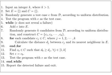
TheFixed-Sized-Candidate-Set ART (FSCS-ART) (Chen et al., 2004c)

main-tains two sets of test cases. One set is theexecuted set E ={e1, e2,· · · , e_n}, as

defined in the previous section; the other set is the candidate set, which

con-tains k randomly generated inputs, denoted byC={c1, c2,· · · , c_k}, wherek

is fixed throughout the testing process. A candidate will be selected as the

next test case if it has the longest distance to its nearest neighbour in E. Figure 1 shows the FSCS-ART algorithm. In this paper, the default value of

k is set as 10, as recommended by Chen et al. (2004c).

1. Input an integerk, wherek >1. 2. SetE ={} and C={}.

3. Randomly generate a test caseefrom D, according to uniform distribution. 4. Test the program witheas the test case.

5. while (edoes not reveal a failure)

6. Add eintoE.

7. Randomly generatek candidates from D, according to uniform distribu-tion, and constructC={c1, c2,· · ·, ck}.

8. foreach candidate cj ∈C, where j= 1,2,· · · , k

9. Calculate the distance dj between cj and its nearest neighbour inE.

10. end for

11. Find cb ∈C such thatdb ≥dj,∀j∈[1, k]

12. Sete=cb.

13. Test the program witheas the test case.

14. end while

15. Report the detected failure and exit.

Figure 1: The algorithm of FSCS-ART

2.3 RRT

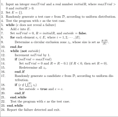
In Restricted Random Testing (RRT) (Chan et al., 2006), anexclusion zone

(8)

E is of the same size R· |D|

|E| , where R is referred to as the target exclusion

ratio. The RRT algorithm continuously generates inputs randomly from D

until an input is generated outside all exclusion zones, which is then used as

the next test case. Figure 2 shows details of the RRT algorithm.

1. Input an integermaxT rial and a real number initialR, wheremaxT rial >

0 and initialR >0. 2. SetE ={}.

6. Add eintoE.

7. SetnoT rial= 0,R=initialR, andoutside= false. 8. foreach element ei ∈E, where i= 1,2,· · · ,|E|.

9. Determine a circular exclusion zonezi, whose size is set as R_|·|D|_E_| .

10. end for

11. while (not outside)

12. IncrementnoT rial by 1.

13. if (noT rial=maxT rial)

14. SetnoT rial= 0 and R=R−0.1 (ifR <0, then setR= 0).

15. Redetermine allzi.

16. end if

17. Randomly generate a candidatec from D, according to uniform dis-tribution.

18. if (c /∈S|_iE=1| zi)

19. Setoutside=true and e=c.

20. end if

21. end while

23. end while

24. Report the failure detected and exit.

Figure 2: The algorithm of RRT

Some simulations (Chan et al., 2006) have shown that the

(9)

Con-sequently, a larger R may result in a longer computation time to find an appropriate test case. Previous studies have assumed a constant R. In this paper, two parameters (initialR and maxT rial) were introduced to provide a facility that can dynamically reduce the value of R as a trade-off between the computation time and the even spreading of test cases. At first, R is set to be equal to initialR. If the RRT algorithm cannot find any appropriate input as the next test case after maxT rial attempts, R will be reduced by a certain value (the reduction step value is set as 0.1 in this study). In this

pa-per, we will use 1.0, 1.7, 3.3 and 6.4 as the default values of initialR for 1D, 2D, 3D and 4D RRT, respectively, as recommended by Chan et al. (2006).

The algorithms in both Figures 1 and 2 are specifically used to evaluate

the F-measure of ART. Therefore, the termination condition (“e does not reveal a failure” on Line 5 in Figures 1 and 2), is effectively set as “when the

first failure is detected”. It should be noted that when these ART algorithms

are applied in real life, there are other possible termination conditions, such

as “when a certain number of test cases have been selected”, “when testing

resources are exhausted”, etc.

2.4 Edge preferences of FSCS-ART and RRT

Chen et al. (2007c) have pointed out that both FSCS-ART and RRT prefer

to select test cases from the edge part of Drather than from the central part.

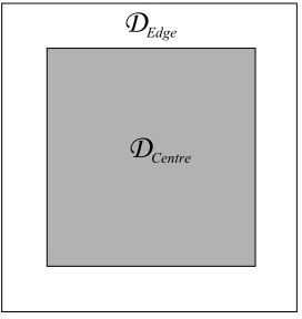
Chen et al. (2007c) measured the edge preference of an ART algorithm by

a metric, namely MEdge:Centre, which is defined as the ratio of the number

of test cases inside the subdomain DEdge to the number of test cases inside

the subdomain DCentre, where DCentre is located in the centre of D, DEdge is

right outsideDCentre, and the sizes ofDCentreandDEdgeare equal. These two

(10)

values of MEdge:Centre for FSCS-ART and RRT are always greater than 1,

and the edge preference of RRT is more significant than that of FSCS-ART.

D

_Centre

D

_Edge

Figure 3: DEdge and DCentre in a 2D space

Some testing methods, such as the domain testing strategy (White and

Cohen, 1980) and boundary-value analysis (Myers, 2004), select test cases

close to or exactly on some “borders”. However, the concept of “border” in

these testing methods is different from the concept of “edge” in this study.

For example, in the domain testing strategy, testers first divideDinto regions

based on the execution paths of the program under test. Test cases are then

selected from near or on the borders of these regions. Obviously, these borders

are not necessarily the boundary of D. However, in FSCS-ART and RRT,

the edge means the boundary of D.

3 Measuring the Edge preference of an ART

Algorithm

MEdge:Centreonly coarsely measures the edge preference of an ART algorithm

(11)

the edge preference of an ART algorithm by a graph, namely the frequency

distribution graph of test cases with respect to the edge and the centre of D

(abbreviated as ECgraph). The method of getting the ECgraphof an ART algorithm is as follows.

(1) Partition D into m equal-sized and disjoint subdomains (denoted by Di, where i = 1,2,· · · , m) from the edge (where i = 1) to the centre

(wherei=m) ofD. Figure 6 illustrates the partitioning in a 2D space. In Figure 6,D is partitioned intoD1,D2,D3 and D4, which are located

from the edge to the centre of D, respectively, and have the same size.

(2) Generate a set of test cases.

(3) Record the number of points in each subdomain.

(4) Calculate the normalized frequency of test cases in each subdomain.

(5) Repeat Steps (2)-(4) for a sufficient number of times to obtain reliable

average values of frequencies with a confidence level of 95% and ±5%

accuracy range.

(6) Plot a curve in a 2D coordinate system, where the x-axis lists all

subdo-mains from the edge (D1) to the centre (Dm) of D, and y-axis denotes

the normalized frequency of test cases inside each subdomain.

Based on the average values of normalized frequencies in the ECgraph, two more statistical data can be collected, (i) the standard deviation of av-erage normalized frequencies, denoted by MEC−SD, and (ii) the difference

between the maximal and minimal values of average normalized

(12)

MEC−M M are, the more uniformly an ART algorithm distributes its test

cases.

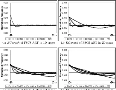
We conducted a series of simulations to obtain ECgraphs of pure RT, FSCS-ART and RRT in 1D, 2D, 3D and 4D spaces. In these simulations,

we setm = 128, because such a value ensures a sufficiently preciseECgraph

at an acceptable computation overhead. Furthermore, many previous

stud-ies (Merkel, 2005; Mayer and Schneckenburger, 2006; Chen et al., 2007a)

have also used such a value for plotting the spatial distribution of test cases;

and our setting will make it easier to compare different works in the

fu-ture. |E| was set as 10, 100, 1000, and 10000. The simulation results are shown in Figures 4 and 5. It has been observed that no matter what |E| is, the normalized frequency for RT is always around 1/128 (that is, 1/m), as theoretically expected, that is, the test cases of RT are always uniformly

distributed. Therefore, in these figures, we only plot the ECgraph of RT with |E|= 10000.

The values ofMEC−SD and MEC−M M for RT, FSCS-ART, and RRT are

summarized in Table 1.

Table 1: Values of MEC−SD and MEC−M M for RT, FSCS-ART, and RRT

dimension testing strategy |E| = 10 |E| = 100 |E| = 1000 |E| = 10000 MEC-SD MEC-MM MEC-SD MEC-MM MEC-SD MEC-MM MEC-SD MEC-MM

1D RT 8.56E-05 4.01E-04 2.95E-05 1.56E-04 1.78E-04 9.30E-04 6.09E-05 2.98E-04 FSCS-ART 1.67E-03 1.16E-02 4.08E-04 5.10E-03 9.59E-05 6.55E-04 2.02E-05 9.75E-05 RRT 1.44E-03 9.51E-03 3.85E-04 4.84E-03 8.63E-05 6.40E-04 2.28E-05 1.23E-04 2D RT 9.00E-05 5.54E-04 2.67E-05 1.23E-04 2.10E-04 9.15E-04 6.11E-05 3.36E-04 FSCS-ART 3.13E-03 1.13E-02 1.79E-03 9.70E-03 1.05E-03 9.05E-03 5.62E-04 6.77E-03 RRT 3.47E-03 1.25E-02 2.62E-03 1.54E-02 1.62E-03 1.53E-02 8.94E-04 1.14E-02 3D RT 9.33E-05 4.30E-04 2.99E-05 1.47E-04 2.08E-04 9.80E-04 5.87E-05 3.06E-04 FSCS-ART 3.57E-03 1.12E-02 2.72E-03 1.00E-02 2.01E-03 9.44E-03 1.41E-03 9.23E-03 RRT 4.52E-03 1.49E-02 4.95E-03 2.05E-02 3.88E-03 2.24E-02 2.74E-03 2.09E-02 4D RT 9.36E-05 4.33E-04 2.80E-05 1.34E-04 2.08E-04 1.29E-03 5.51E-05 2.78E-04 FSCS-ART 3.74E-03 1.23E-02 3.21E-03 1.05E-02 2.70E-03 1.01E-02 2.16E-03 9.69E-03 RRT 5.02E-03 1.63E-02 6.28E-03 2.28E-02 5.53E-03 2.38E-02 4.37E-03 2.29E-02

(13)

0.000 0.005 0.010 0.015 0.020 0.025 0.030 128 121 114 107 100 93 86 79 72 65 58 51 44 37 30 23 16 9 2 N o rm a li ze d F re q u e n c y

|E|=10 |E|=100 |E|=1000 |E|=10000 RT D1 … … … … D128

4.a ECgraphof FSCS-ART in 1D space

|E|=10 |E|=100 |E|=1000 |E|=10000 RT D1 … … … … D128

4.b ECgraphof FSCS-ART in 2D space

|E|=10 |E|=100 |E|=1000 |E|=10000 RT D1 … … … … D128

4.c ECgraph of FSCS-ART in 3D space

|E|=10 |E|=100 |E|=1000 |E|=10000 RT D1 … … … … D128

4.d ECgraphof FSCS-ART in 4D space

Figure 4: Frequency distribution of test cases selected by FSCS-ART with respect to the edge and the centre of input domain

(1) Both FSCS-ART and RRT have an edge preference.

(2) The edge preference becomes more significant with the increase of the

dimension of D.

(3) The edge preference becomes less significant with the increase of |E|.

(4) The edge preference of RRT is more significant than that of FSCS-ART

for high dimension cases.

FSCS-ART and RRT algorithms evenly spread test cases by enforcing

them far apart from one another; as a consequence, some of their test cases

(14)

|E|=10 |E|=100 |E|=1000 |E|=10000 RT D1 … … … … D128

5.a ECgraphof RRT in 1D space

|E|=10 |E|=100 |E|=1000 |E|=10000 RT D1 … … … … D128

5.b ECgraphof RRT in 2D space

|E|=10 |E|=100 |E|=1000 |E|=10000 RT D1 … … … … D128

5.c ECgraph of RRT in 3D space

|E|=10 |E|=100 |E|=1000 |E|=10000 RT D1 … … … … D128

5.d ECgraphof RRT in 4D space

Figure 5: Frequency distribution of test cases selected by RRT with respect to the edge and the centre of input domain

a by-product of the test case selection procedures of FSCS-ART and RRT.

However, it was observed that a poor failure-detection capability is always

associated with a significant edge preference. As shown in the above

ex-perimental data, the edge preferences of FSCS-ART and RRT become more

significant as |E| decreases or the dimension of D increases. It was also re-ported that FSCS-ART and RRT have poorer failure detection capabilities

for the cases of higher θ or higher dimension (Chen et al., 2007c). Such a correlation between the edge preference and the effectiveness of these ART

algorithms has motivated us to improve these algorithms by offsetting their

(15)

4 Enhancing ART by offsetting the Edge

preference

In this section, we will introduce a new approach to offsetting the edge

pref-erence of FSCS-ART and RRT algorithms. In this approach,Dis partitioned

into some equal-sized partitions from the edge to the centre of D, and test

cases will be evenly selected from these partitions. We integrate such a

Partitioning by Edge and Centre (ECP) approach with the existing ART

al-gorithms, and develop a new family of ART alal-gorithms, namely ECP-ART

algorithms. The new algorithms and their performances are elaborated in

the following sections.

4.1 ART with partitioning by edge and centre

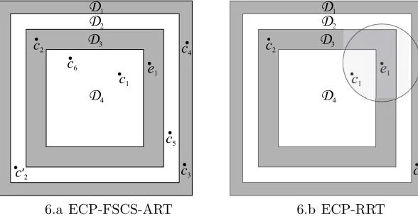
There are two instances of ART algorithms, FSCS-ART and

ECP-RRT, which will be illustrated in a 2D space, as shown in Figures 6.a and 6.b,

respectively. In these figures,D is partitioned into four equal-sized partitions

D1, D2, D3 and D4, from the edge to the centre, respectively.

D₄

D3

D2

D₁

c2

c5 c₄

c_’₂

c₆

c3 e1 c1

6.a ECP-FSCS-ART

c2

c3

e1

c1

D₄

D3

D2

D₁

6.b ECP-RRT

(16)

ECP-FSCS-ART is an integration of the ECP approach and FSCS-ART

algorithm. Figure 6.a illustrates how it works. Suppose that the first test

case e1 is randomly generated from D and happens to be located inside D3.

With regard to the selection of the next test case, six candidates,c1,c2,c3,c4,

c5 and c6, are generated, as shown in Figure 6.a. However, since c2 is inside

the same partition as e1, ECP-FSCS-ART requires a random replacement

for c2, sayc′2 which is not located inside the same partition ase1. Then, the

second test case e2 is selected from c1, c′2 (instead of c2), c3, c4, c5 and c6.

Since c′

2 is the farthest candidate from e1, it will be selected as e2.

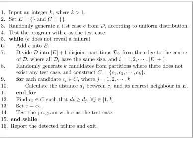
For ECP-RRT (the integration of the ECP approach and RRT algorithm),

refer to Figure 6.b. Suppose that the first random test case e1 resides inside

D3. A random inputc1 is generated and found to be inside the exclusion zone

of e1 (the shadowed circular zone around e1). c1 will be discarded, and then

another input c2 will be randomly generated, which happens to be outside

the exclusion zone ofe1. Unfortunately,c2is in the same partition ase1 (that

is, D3). ECP-RRT will discard c2, and then c3 will be generated. c3 will be

selected as the next teste2, because it is both outside the exclusion zone and

the partition of e1.

4.1.1 Details of new algorithms

There are two methods to implement the ECP approach. One method is to

dynamically partition D, that is, the number of partitions is varying with

the number of executed test cases. The other method is static partitioning,

that is, the number of partitions is fixed throughout the testing process. As

reported by Chen et al. (2007b), the dynamic partitioning method performs

better than the static method. Therefore, in this paper, we will focus on

(17)

of ECP-FSCS-ART and ECP-RRT algorithms are given in Figures 7 and 8,

respectively.

1. Input an integerk, wherek >1. 2. SetE ={} and C={}.

6. Add eintoE.

7. DivideD into|E|+ 1 disjoint partitionsDi, from the edge to the centre

of D, where allDi have the same size, andi= 1,2,· · ·,|E|+ 1.

8. Randomly generatek candidates from partitions where there does not exist any test case, and constructC ={c1, c2,· · · , c_k}.

9. foreach candidate cj ∈C, where j= 1,2,· · · , k

10. Calculate the distance dj betweencj and its nearest neighbour inE.

11. end for

12. Find cb ∈C such thatdb ≥dj,∀j∈[1, k]

13. Sete=cb.

15. end while

16. Report the detected failure and exit.

Figure 7: The algorithm of ECP-FSCS-ART

As shown in Figures 7 and 8, ECP-ART always has |E|+ 1 partitions. Therefore, at least one partition will not contain any executed test case. Our

approach is to select the next test case from a “blank” partition. This will

prevent test cases from being selected more frequently in certain subdomains,

and hence offset the edge preference.

4.1.2 Runtime of new algorithms

Since the new algorithms are the integration of the ECP approach and the

original ART algorithms, we will only analyze the computational overhead

(18)

1. Input an integermaxT rial and a real number initialR, wheremaxT rial >

0 and initialR >0. 2. SetE ={}.

6. Add eintoE.

7. DivideD into|E|+ 1 disjoint partitionsDi, from the edge to the centre

of D, where allDi have the same size, andi= 1,· · · ,|E|+ 1.

8. SetnoT rial= 0,R=initialR, andoutside= false. 9. foreach element ei ∈E, where i= 1,2,· · · ,|E|.

10. Determine a circular exclusion zone zi, whose size is set as R_|·|D|_E_| .

11. end for

12. while (not outside)

13. Increment noT rialby 1.

14. if (noT rial=maxT rial)

15. SetnoT rial= 0 and R=R−0.1 (ifR <0, then setR= 0).

16. Redetermine allzi.

17. end if

18. Randomly generate a candidate cfrom partitions where there does

not exist any executed test case. 19. if (c /∈S|_iE=1| zi)

20. Setoutside=true and e=c.

21. end if

22. end while

24. end while

25. Report the failure detected and exit.

(19)

the ECP approach will first partitionD into|E|+ 1 partitions; then identify the blank partitions, that is, the partitions which do not contain any executed

test case; and finally, generate candidates from the blank partitions. Since

D is of numeric type, it is very easy to calculate the value ranges for all

partitions. For each executed test case, its corresponding partition can be

identified simply through checking which value range each of its coordinates

belongs to. Therefore, the identification of blank partitions requires O(|E|) time. With regard to the candidate generation, it is basically the same

as the random generation of any possible program input, except that the

candidate must be selected within the value range of a blank partition Di

instead of from D. Briefly speaking, it takes O(|E|) time to implement the ECP approach in the process of selecting the (|E|+ 1)th test case, and thus the total computation overhead of the ECP approach for selecting |E| test cases is in O(|E|2

). Since FSCS-ART and RRT algorithms require O(|E|2

)

and O(|E|2

log|E|) time to select |E| test cases, respectively (Mayer and Schneckenburger, 2006), the orders of computation of ECP-ART and the

original ART algorithms are the same.

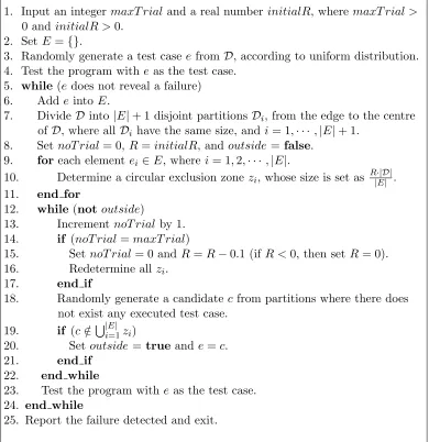
We also experimentally evaluated the runtime of ECP-ART via some

simulations. All simulations were conducted on a machine with an Intel

Pentium processor running at 3195 MHz and 1024 megabytes of RAM. The

ART algorithms were implemented in C language and compiled with GNU

Compiler Collection (version 3.3.4) (GCC, 2004). FSCS-ART,

ECP-FSCS-ART, RRT, and ECP-RRT were implemented in a 2D space. For each

al-gorithm, we recorded the time taken to select a number of test cases, with

|E|= 500,1000,1500,2000,2500, and 3000. The simulation results are given in Figure 9, in which, x- and y-axes denote|E|and time required to generate

(20)

both requireO(|E|2

) time to select|E|test cases, while the runtimes of RRT and ECP-RRT are both in O(|E|2

log|E|). In other words, the experimental data are consistent with the theoretical analysis.

0 10 20 30 40 50 60

500 1000 1500 2000 2500 3000

|E|

g

e

n

e

ra

ti

o

n

t

im

e

(

s

e

c

o

n

d

s

)

FSCS-ART ECP-FSCS-ART

RRT ECP-RRT

Figure 9: Comparison of runtime between the original ART algorithms and the new ECP-ART algorithms

4.2 Experiment 1

The intuition of ART is to enforce random test cases as evenly spread as

possible. Thus, it is important to know how evenly ECP-ART algorithms

spread their test cases. Chen et al. (2007c) have used three metrics to

(21)

these metrics, MEdge:Centre has been discussed in Section 2.4. The other two

metrics are discrepancy and dispersion, which are commonly used in

measur-ing the equidistribution of sample points (Branicky et al., 2001). Intuitively

speaking, discrepancy indicates whether regions have an equal density of the

points; while dispersion indicates whether any point in E is surrounded by a very large empty spherical region (containing no points other than itself).

E is considered reasonably equidistributed if discrepancy is close to 0, dis-persion is small, andMEdge:_Centre is close to 1 (that is, the edge preference is

insignificant).

We first examine to what extent ECP-ART algorithms offset the edge

preference. We repeated the simulations in Section 3 using ECP-FSCS-ART

and ECP-RRT. The simulations results are shown in Figures 10 and 11,

respectively. The values ofMEC−SD and MEC−M M for ECP-FSCS-ART and

ECP-RRT are summarized in Table 2.

Table 2: Values of MEC−SD and MEC−M M for FSCS-ART and

ECP-RRT

dimension testing strategy |E| = 10 |E| = 100 |E| = 1000 |E| = 10000 MEC-SD MEC-MM MEC-SD MEC-MM MEC-SD MEC-MM MEC-SD MEC-MM

1D ECP-FSCS-ART 1.35E-03 9.65E-03 1.06E-04 7.77E-04 6.86E-05 3.15E-04 2.07E-05 1.22E-04 ECP-RRT 1.02E-03 1.07E-02 1.76E-04 8.03E-03 7.85E-05 8.01E-03 2.11E-05 7.85E-03 2D ECP-FSCS-ART 8.54E-04 3.13E-03 3.83E-04 2.22E-03 2.83E-04 2.22E-03 8.74E-05 7.64E-04 ECP-RRT 9.97E-04 9.94E-03 8.14E-04 1.06E-02 4.98E-04 1.07E-02 2.88E-04 1.06E-02 3D ECP-FSCS-ART 1.37E-03 4.07E-03 6.68E-04 2.58E-03 4.26E-04 2.38E-03 2.65E-04 2.08E-03 ECP-RRT 1.28E-03 1.01E-02 1.66E-03 1.12E-02 1.23E-03 1.16E-02 8.49E-04 1.17E-02 4D ECP-FSCS-ART 1.68E-03 4.80E-03 9.42E-04 2.98E-03 6.16E-04 2.84E-03 4.18E-04 2.30E-03 ECP-RRT 1.86E-03 1.01E-02 2.23E-03 1.14E-02 1.82E-03 1.17E-02 1.38E-03 1.17E-02

Based on these data, we make the following three observations.

(1) ECP-ART algorithms distribute test cases more evenly than the

origi-nal ART algorithms. Moreover, by comparing Figures 4 and 10 as well

as Figures 5 and 11, it can be further observed that ECP-ART

(22)

|E|=10 |E|=100 |E|=1000 |E|=10000 RT D1 … … … … D128

10.a ECgraph of ECP-FSCS-ART in 1D space 0.000 0.005 0.010 0.015 0.020 0.025 0.030 128 121 114 107 100 93 86 79 72 65 58 51 44 37 30 23 16 9 2 N o rm a li ze d F re q u e n c y

|E|=10 |E|=100 |E|=1000 |E|=10000 RT D1 … … … … D128

10.b ECgraph of ECP-FSCS-ART in 2D space 0.000 0.005 0.010 0.015 0.020 0.025 0.030 128 121 114 107 100 93 86 79 72 65 58 51 44 37 30 23 16 9 2 N o rm a li ze d F re q u e n c y

|E|=10 |E|=100 |E|=1000 |E|=10000 RT D1 … … … … D128

10.c ECgraph of ECP-FSCS-ART in 3D space 0.000 0.005 0.010 0.015 0.020 0.025 0.030 128 121 114 107 100 93 86 79 72 65 58 51 44 37 30 23 16 9 2 N o rm a li ze d F re q u e n c y

|E|=10 |E|=100 |E|=1000 |E|=10000 RT D1 … … … … D128

10.d ECgraph of ECP-FSCS-ART in 4D space

Figure 10: Frequency distribution of test cases selected by ECP-FSCS-ART with respect to the edge and the centre of input domain

RRT have a higher edge preference.

(2) There is still a small edge preference for ECP-ART algorithms.

(3) Based on Table 2, it can be observed that when the dimension of D is

higher than 1, ECP-FSCS-ART algorithm has a smaller edge preference

than ECP-RRT algorithm.

The first observation is consistent with the intuition of our study, that

is, the edge preference can be offset by ECP-ART algorithms. It has been

(23)

|E|=10 |E|=100 |E|=1000 |E|=10000 RT D1 … … … … D128

11.aECgraph of ECP-RRT in 1D space

|E|=10 |E|=100 |E|=1000 |E|=10000 RT D1 … … … … D128

11.b ECgraph of ECP-RRT in 2D space

|E|=10 |E|=100 |E|=1000 |E|=10000 RT D1 … … … … D128

11.cECgraph of ECP-RRT in 3D space

|E|=10 |E|=100 |E|=1000 |E|=10000 RT D1 … … … … D128

11.d ECgraph of ECP-RRT in 4D space

Figure 11: Frequency distribution of test cases selected by ECP-RRT with respect to the edge and the centre of input domain

more significant edge preference of FSCS-ART and RRT. Therefore, it is

expected that ECP-ART algorithms have a more noticeable offset of the

edge preference when the dimension is higher or θ is higher. The second observation can be explained as follows. Although the next test case is from

a “blank” partition, there can be more than one blank partition. Due to

the nature of FSCS-ART and RRT, inputs from the blank partition near

D’s edge have a higher probability to be selected as the next test case than

inputs from the blank partition near D’s centre. The last observation is also

understandable. Since the edge preference of the original RRT algorithm

(24)

dimension ofDis high, it is intuitive for ECP-RRT to have a more significant

edge preference than ECP-FSCS-ART for higher dimensions.

In order to further investigate the test case distributions of ECP-ART

algorithms, we repeated the simulations in the study of Chen et al. (2007c) on

ECP-FSCS-ART and ECP-RRT, and got their discrepancies and dispersions.

Since we found that ECP-RRT distributes test cases similarly as

ART, we only report the values of discrepancy and dispersion for

ECP-FSCS-ART, as shown in Figures 12 and 13, respectively. For ease of comparison, the

previous simulation results of FSCS-ART are also included in these figures.

These figures clearly show that ECP-FSCS-ART has a smaller MDiscrepancy

than FSCS-ART, and its MDispersion is similar to that of FSCS-ART.

0.00 0.01 0.02 0.03 0.04 0.05 0.06 0.07 0.08 0.09

0 2000 4000 6000 8000 10000

|E| D is c re p a n c y FSCS-ART ECP-FSCS-ART 12.a discrepancy in 1D space

0.00 0.01 0.02 0.03 0.04 0.05 0.06 0.07 0.08 0.09

0 2000 4000 6000 8000 10000

|E| D is c re p a n c y FSCS-ART ECP-FSCS-ART 12.b discrepancy in 2D space

0.00 0.01 0.02 0.03 0.04 0.05 0.06 0.07 0.08 0.09

0 2000 4000 6000 8000 10000

|E| D is c re p a n c y FSCS-ART ECP-FSCS-ART 12.c discrepancy in 3D space

0.00 0.01 0.02 0.03 0.04 0.05 0.06 0.07 0.08 0.09

0 2000 4000 6000 8000 10000

|E| D is c re p a n c y FSCS-ART ECP-FSCS-ART 12.d discrepancy in 4D space

(25)

0.00 0.07 0.14 0.21 0.28 0.35 0.42

0 2000 4000 6000 8000 10000

|E|

D

is

pe

rs

ion

FSCS-ART ECP-FSCS-ART 13.a dispersion in 1D space

0.00 0.07 0.14 0.21 0.28 0.35 0.42

0 2000 4000 6000 8000 10000

|E|

D

is

pe

rs

ion

FSCS-ART ECP-FSCS-ART 13.b dispersion in 2D space

0.00 0.07 0.14 0.21 0.28 0.35 0.42

0 2000 4000 6000 8000 10000

|E|

D

is

pe

rs

ion

FSCS-ART ECP-FSCS-ART 13.c dispersion in 3D space

0.00 0.07 0.14 0.21 0.28 0.35 0.42

0 2000 4000 6000 8000 10000

|E|

D

is

p

e

rs

io

n

FSCS-ART ECP-FSCS-ART 13.d dispersion in 4D space

Figure 13: Comparison of dispersion between ECP-ART and FSCS-ART

In summary, ECP-ART algorithms can offset the edge preference very

well, and spread test cases more evenly than the original ART algorithms.

4.3 Experiment 2

The previous section concludes that the new ECP-ART algorithms distribute

test cases more evenly than original ART algorithms. We are now going to

examine whether the failure detection capabilities can be improved, through a

series of simulations. The parameters for these simulations are set as follows.

(26)

• θ: 0.75, 0.5, 0.25, 0.1, 0.075, 0.05, 0.025, 0.01, 0.0075, 0.005, 0.0025, 0.001, 0.00075, 0.0005, 0.00025, 0.0001, 0.000075, and 0.00005.

• Failure pattern: a single square failure region is randomly placed inside

D.

It should be noted that the setting of this experiment is exactly the

same as Experiment 1 in the study of Chen et al. (2007d). The results of

these simulations are reported in Figure 14, which also includes the previous

simulation results of FSCS-ART and RRT for ease of comparison. Note that

the scales in Figure 14 do not start at 0.

0.5 0.6 0.7 0.8 0.9 1.0 1.1 1.00E-05 1.00E-04 1.00E-03 1.00E-02 1.00E-01 1.00E+00 T ART F -rat io = F A R T / F R T

FSCS-ART ECP-FSCS-ART RRT ECP-RRT 14.a Comparison in 1D space

0.5 0.6 0.7 0.8 0.9 1.0 1.1 1.2 1.00E-05 1.00E-04 1.00E-03 1.00E-02 1.00E-01 1.00E+00 T ART F -rat io = F A R T / F R T

FSCS-ART ECP-FSCS-ART RRT ECP-RRT 14.b Comparison in 2D space

0.6 0.7 0.8 0.9 1.0 1.1 1.2 1.3 1.4 1.5 1.00E-05 1.00E-04 1.00E-03 1.00E-02 1.00E-01 1.00E+00 T ART F -rat io = F A R T / F R T

FSCS-ART ECP-FSCS-ART RRT ECP-RRT 14.c Comparison in 3D space

0.7 0.8 0.9 1.0 1.1 1.2 1.3 1.4 1.5 1.6 1.7 1.8 1.9 2.0 2.1 1.00E-05 1.00E-04 1.00E-03 1.00E-02 1.00E-01 1.00E+00 T ART F -rat io = F A R T / F R T

FSCS-ART ECP-FSCS-ART RRT ECP-RRT 14.d Comparison in 4D space

Figure 14: Comparison of failure detection capabilities between the original ART algorithms and the new ECP-ART algorithms

(27)

(1) When the dimension ofD orθ is high, the failure detection capabilities of ECP-ART algorithms are better than those of the original ART

algorithms; otherwise, the performances of ECP-ART and the original

ART algorithms are more or less similar.

(2) ECP-FSCS-ART is more effective than ECP-RRT for the cases of high

dimension and high θ.

The first conclusion is expected. As explained in Section 4.2, the higher

the dimension of D orθ is, the more edge preference will be offset by ECP-ART algorithms. Since ECP-ECP-ART algorithms are introduced to enhance the

failure detection capabilities of the original ART algorithms by offsetting

their edge preferences, it is expected that the higher the dimension ofDorθ, the better improvement of the failure-detection capability of ECP-ART over

the original ART algorithms. It is also understandable to have the second

conclusion that ECP-FSCS-ART has better failure-detection capability than

ECP-RRT for higher θ cases, because the former can distribute test cases more evenly than the latter (the last observation in Section 4.2).

As a summary of experiments reported in Sections 4.2 and 4.3, the new

partitioning approach enhances the original ART algorithms not only in

terms of the even distribution of test cases, but also with respect to the

failure-detection capability. As shown in these experiments,

ECP-FSCS-ART and ECP-RRT algorithms have similar performance trends, so we will

only investigate ECP-FSCS-ART in the rest of the experimental study.

4.4 Experiment 3

(28)

compact the failure region is, (b) how many failure regions there are, (c) whether there exists a predominant failure region by size, and (d) how large the predominant failure region is. In this section, we conducted a similar

investigation for ECP-FSCS-ART.

We first conducted a simulation to see how the compactness of a failure

region influences the failure-detection capability of ECP-FSCS-ART. The

simulation used the rectangle (instead of the square in Section 4.3) as the

shape of the failure region in order to investigate the impact of compactness.

The experimental setting is as follows.

• Dimension of D: 2, 3 and 4.

• θ: 0.005.

• Failure pattern: a single rectangular region is randomly placed inside

the input domain. The ratios among edge lengths of the rectangular

region are 1 : α, 1 : α : α and 1 : α : α : α in 2D, 3D and 4D spaces, respectively, where α≥1.

• α: 1, 4, 7, 10, 20, 30, 40, 50, 60, 70, 80, 90 and 100. As justified by Chen et al. (2007d), the larger α is, the less compact the failure region is.

The above experimental setting is similar to the setting of Experiment 2

in the study of Chen et al. (2007d). The simulation results are reported in

Figure 15, which also includes the previous simulation results on FSCS-ART

for ease of comparison. As shown in Figure 15, although the effectiveness of

FSCS-ART also depends on the compactness of a failure region,

ECP-FSCS-ART outperforms ECP-FSCS-ART in most scenarios, and the performance

(29)

0.6 0.7 0.8 0.9 1.0 1.1 1.2 1.3

0 10 20 30 40 50 60 70 80 90 100

D A RT F -rati o = F A R T / F R T FSCS-ART ECP-FSCS-ART 15.a 2D,θ= 0.005

0.6 0.7 0.8 0.9 1.0 1.1 1.2 1.3

0 10 20 30 40 50 60 70 80 90 100

D A RT F -rati o = F A R T / F R T FSCS-ART ECP-FSCS-ART 15.b 3D,θ= 0.005

0.6 0.7 0.8 0.9 1.0 1.1 1.2 1.3

0 10 20 30 40 50 60 70 80 90 100

D A RT F -rati o = F A R T / F R T FSCS-ART ECP-FSCS-ART 15.c 4D,θ= 0.005

Figure 15: Failure detection capabilities of ECP-FSCS-ART on a rectangular failure region

We conducted another simulation to evaluate the failure-detection

capa-bility of ECP-FSCS-ART where there are more than one failure region. The

experimental setting of this simulation is as follows.

• θ: 0.005.

• Failure pattern: a number of equal-sized square regions are randomly

placed inside the input domain.

• The number of failure regions: 1, 4, 7, 10, 20, 30, 40, 50, 60, 70, 80, 90

(30)

It should be noted that the above setting is similar to the experimental

setting of Experiment 3 in the study of Chen et al. (2007d). Figure 16 shows

the simulation results. It can be observed that ECP-FSCS-ART behaves

similarly as FSCS-ART, that is, its effectiveness depends on the number of

failure regions. But ECP-FSCS-ART has a better failure-detection

capabil-ity, especially when the dimension of D is higher.

0.6 0.7 0.8 0.9 1.0 1.1 1.2 1.3

0 10 20 30 40 50 60 70 80 90 100

Number of failure regions

A RT F -rati o = F A R T / F R T FSCS-ART ECP-FSCS-ART 16.a 2D,θ= 0.005

0.6 0.7 0.8 0.9 1.0 1.1 1.2 1.3

0 10 20 30 40 50 60 70 80 90 100

A RT F -rati o = F A R T / F R T FSCS-ART ECP-FSCS-ART 16.b 3D,θ= 0.005

0.6 0.7 0.8 0.9 1.0 1.1 1.2 1.3

0 10 20 30 40 50 60 70 80 90 100

A RT F -rat io = F A R T / F R T FSCS-ART ECP-FSCS-ART 16.c 4D,θ= 0.005

Figure 16: Failure detection capabilities of ECP-FSCS-ART on multiple equal-sized failure regions

In the above simulation, all the failure regions have the same size.

How-ever, it is unlikely that all failure regions are equal-sized in reality. Therefore,

we further conducted a simulation where failure regions are of different sizes.

(31)

• θ: 0.005.

• Failure pattern: a number of square regions are randomly placed

in-side the input domain. Suppose that there are n failure regions, denoted by R1, R2,· · · , Rn, respectively. The sizes of these regions

(|R1|,|R2|,· · · ,|R_n|) are assigned by either of the following two ways.

* Existence of a predominant failure region. For one region Rn, set

|Rn| = r ·θ · |D|, where r = 0.3,0.5 and 0.8. For all the other

regions, |Ri| = vi

Pn−1

i=1 vi

·(1−r)·θ · |D|, where vi is a random

number uniformly distributed in [0,1), andi= 1,2,· · · , n−1.

* No predominant failure region. For all regions, |Ri|= vi

Pn i=1vi

·θ· |D|, where vi is a random number uniformly distributed in [0,1),

and i= 1,2,· · · , n.

• The number of failure regions: 1, 4, 7, 10, 20, 30, 40, 50, 60, 70, 80, 90

and 100.

The above setting is similar to the setting of Experiment 4 in the study

of Chen et al. (2007d). The simulation results of ECP-FSCS-ART as well as

the previous results of FSCS-ART are given in Figure 17. We can observe

that the performance of ECP-FSCS-ART also depends on the existence and

the size of a predominant failure region, and ECP-FSCS-ART generally has

a better failure-detection capability than the original FSCS-ART.

Based on experiments reported in Sections 4.3 and 4.4, we conclude that

like FSCS-ART, the failure-detection capability of ECP-FSCS-ART also

(32)

0.6 0.7 0.8 0.9 1.0 1.1 1.2 1.3

0 10 20 30 40 50 60 70 80 90 100

A RT F -rati o = F A R T / F R T FSCS-ART ECP-FSCS-ART 17.a No predominant failure region, 2D

0.6 0.7 0.8 0.9 1.0 1.1 1.2 1.3

0 10 20 30 40 50 60 70 80 90 100

A RT F -rati o = F A R T / F R T FSCS-ART ECP-FSCS-ART

17.d Predominant failure region exists, 2D,

r= 0.3

0.6 0.7 0.8 0.9 1.0 1.1 1.2 1.3

0 10 20 30 40 50 60 70 80 90 100

A RT F -rati o = F A R T / F R T FSCS-ART ECP-FSCS-ART 17.b No predominant failure region, 3D

0.6 0.7 0.8 0.9 1.0 1.1 1.2 1.3

0 10 20 30 40 50 60 70 80 90 100

17.e Predominant failure region exists, 3D,

r= 0.3

0.6 0.7 0.8 0.9 1.0 1.1 1.2 1.3

0 10 20 30 40 50 60 70 80 90 100

A RT F -rat io = F A R T / F R T FSCS-ART ECP-FSCS-ART 17.c No predominant failure region, 4D

0.6 0.7 0.8 0.9 1.0 1.1 1.2 1.3

0 10 20 30 40 50 60 70 80 90 100

A RT F -rat io = F A R T / F R T FSCS-ART ECP-FSCS-ART

17.f Predominant failure region exists, 4D,

(33)

0.6 0.7 0.8 0.9 1.0 1.1 1.2 1.3

0 10 20 30 40 50 60 70 80 90 100

17.g Predominant failure region exists, 2D,

r= 0.5

0.6 0.7 0.8 0.9 1.0 1.1 1.2 1.3

0 10 20 30 40 50 60 70 80 90 100

17.j Predominant failure region exists, 2D,

r= 0.8

0.6 0.7 0.8 0.9 1.0 1.1 1.2 1.3

0 10 20 30 40 50 60 70 80 90 100

17.h Predominant failure region exists, 3D,

r= 0.5

0.6 0.7 0.8 0.9 1.0 1.1 1.2 1.3

0 10 20 30 40 50 60 70 80 90 100

17.k Predominant failure region exists, 3D,

r= 0.8

0.6 0.7 0.8 0.9 1.0 1.1 1.2 1.3

0 10 20 30 40 50 60 70 80 90 100

17.i Predominant failure region exists, 4D,

r= 0.5

0.6 0.7 0.8 0.9 1.0 1.1 1.2 1.3

0 10 20 30 40 50 60 70 80 90 100

17.l Predominant failure region exists, 4D,

r= 0.8

(34)

regions, the existence and the size of a predominant failure region. But

ECP-FSCS-ART generally outperforms the original ECP-FSCS-ART, and the

perfor-mance improvement becomes more significant when the dimension of Dorθ

is higher.

4.5 Experiment 4

Chen et al. (2004c) have also applied the original FSCS-ART to test some

real-life programs, which are all published programs (ACM, 1980; Press et al.,

1986), and were error-seeded using the technique of mutation (Budd, 1981).

As shown in Section 4.3, the failure-detection capability of ECP-FSCS-ART

is dependent on the dimension of D. Therefore, in this experimental study,

we selected four particular programs as the subject programs with varying

dimensions, namely airy,bessj,plgndr, andel2, whose input domains are 1D,

2D, 3D, and 4D, respectively. The details of these 4 programs are given in

Table 3.

Table 3: Program name, dimension, and seeded errors for each subject pro-gram

Program Dimension Number of seeded errors

AOR ROR SVR CR

airy 1 1

bessj 2 2 1 1

plgndr 3 1 2 2

el2 4 1 3 2 3

AOR arithmatic operator replacement

ROR relational operator replacement

SVR scalar variable replacement

CR constant replacement

For each subject program, Chen et al. (2004c) defined its input domain

(35)

the input domains, they estimated the failure rates (θ) of these programs by finding the F-measures of RT and then applying the formula θ = 1/FRT.

In this study, we aim to investigate the impact of the relative locations of

failure regions on the ART performance. Hence, we kept the same seeded

errors for these subject programs, but modified the relative locations of

fail-ure regions by changing the range values for the input domains. Refer to

Table 4, where airy, bessj, plgndr, and el2 denote the programs on original

input domains (which were defined by Chen et al. (2004c)), while airy new,

bessj new, plgndr new and el2 new denote the programs on newly-defined

input domains. The modification of the input domains only have strong

im-pacts on the locations of failure regions and θ of subject programs; while the basic shapes of the failure regions remain unchanged because the seeded

errors are not changed.

Table 4: The failure rates and failure patterns of subject programs on differ-ent input domains

Program Input domain Failure rate Failure pattern

From To (T)

airy (-5000) (5000) 0.000716 A block in the centre of input domain airy_new (0) (10000) 0.000694 A block on the edge of input domain bessj (2, -1000) (300, 15000) 0.001298 Strips near the edge of input domain bessj_new (-100, -8000) (200, 8000) 0.001279 Strips in the centre of input domain plgndr (10, 0, 0) (500, 11, 1) 0.000368 Strips near the edge of input domain plgndr_new (-300, -6, -1) (300, 6, 1) 0.000965 Strips spanning from the centre

to the edge of input domain el2 (0, 0, 0, 0) (250, 250, 250, 250) 0.000690 Strips near the edge of input domain el2_new (-200,-200,-200,-200) (200, 200, 200, 200) 0.000703 Strips crossing the centre of input domain

We applied the original FSCS-ART algorithm to testairy new,bessj new,

plgndr new and el2 new. The experimental results are shown in Table 5,

which also includes the previous results on airy, bessj, plgndr, and el2. It is

clearly shown that as expected, for the same program, FSCS-ART has fairly

(36)

Table 5: Failure detection capabilities of FSCS-ART on 4 programs with different input domains

Program FSCS-ART F-ratio

original input domains new input domains

airy 0.5786 0.3564

bessj 0.5817 0.8102

plgndr 0.6591 0.8462

el2 0.4798 1.0845

We repeated the experiment by applying ECP-FSCS-ART to test all four

subject programs on both the original and the new input domains. The

experimental results are shown in Table 6. As intuitively expected,

ECP-FSCS-ART performs similarly on the same program under various scenarios.

Table 6: Failure detection capabilities of ECP-FSCS-ART on 4 programs with different input domains

Program ECP-FSCS-ART F-ratio

original input domains new input domains

airy 0.5338 0.5534

bessj 0.6347 0.6717

plgndr 0.7011 0.7456

el2 0.7744 0.8289

In summary, the failure-detection capability of ECP-FSCS-ART is less

dependent on the locations of failure regions than that of FSCS-ART.

5 Discussion and Conclusion

ART was originally proposed as an approach to enhancing the

failure-detection capability of RT. Recent studies have pointed out that some ART

algorithms prefer to select test cases from the edge part of the input domain.

(37)

is not desirable for inputs to have different chances of being selected as test

cases. In this paper, we investigated the edge preferences of FSCS-ART and

RRT, and proposed a new family of algorithms, namely ART with

Partition-ing by Edge and Centre (ECP-ART).

ECP-ART uses an additional partitioning scheme to offset the edge

pref-erence. The new ECP-ART algorithms have the same orders of computation

as the original ART algorithms. Compared with the original ART

algo-rithms, ECP-ART algorithms have similar values of dispersion, but smaller

values of discrepancy. In other words, ECP-ART can spread test cases more

evenly than the original ART algorithms. It has also been observed that

the effectiveness of ECP-ART depends on the same factors as the original

ART algorithms. However, ECP-ART algorithms normally have better

fail-ure detection capabilities under the same conditions, and the performance

enhancement of ECP-ART over the original ART algorithms becomes more

significant with the increase of dimension or failure rate. It has also been

shown by simulations and experimental studies that the failure detection

capabilities of the new ECP-ART algorithms are less dependent on the

loca-tions of failure regions than those of the corresponding ART algorithms. In

summary, the basic idea of our new approach is that for an ART algorithm

which prefers to select test cases from certain locations of the input domain,

we offset the preference by using a specifically designed partitioning scheme.

As a pilot study, this paper only investigated how to apply such an idea

into FSCS-ART and RRT algorithms. Mayer and Schneckenburger (2006)

have pointed out that most ART algorithms have a preference toward test

cases from certain locations of the input domain. For example, ART through

Iterative Partitioning (ART-IP) (Chen et al., 2006) has a similar test case

(38)

exhibits a preference on some small square regions inside the input domain.

Chen et al. (2007c) also observed that ART by Random Partitioning

(ART-RP) (Chen et al., 2004a) has a small centre preference (that is, inputs from

the centre part of the input domain has a high probability of being selected

as test cases). Intuitively speaking, the basic idea of this paper can also

be applied to these ART algorithms, as long as we can find appropriate

partitioning schemes that can offset the preferences of these algorithms. The

ECP approach proposed in this paper is applicable for IP and

ART-RP. For LART and many other ART algorithms (such asMirror ART (Chen

et al., 2004b) and ART by Localization (Chen and Huang, 2004)), since they

have more complicated test case distributions than FSCS-ART and RRT,

further investigations are required to find appropriate partitioning schemes

for them.

There exists one particular ART algorithm, namely ART by Bisection

(ART-B) (Chen et al., 2004a), which does not exhibit any preference in

the test case selection. Chen et al. (2007c) have observed that FSCS-ART

and RRT only outperform ART-B when the failure rate is small. We have

compared the failure detection capabilities of ART-B and ECP-ART, and

found that ECP-ART normally has a better failure-detection capability than

ART-B, no matter whether the failure rate is high or not.

In conclusion, this paper has proposed a new approach that can help some

ART algorithms spread test cases more evenly and detect software failures

more effectively. The basic idea of the new approach is not only applicable

(39)

Acknowledgment

This research project is supported by an Australian Research Council

Dis-covery Grant (DP0880295).

References

ACM, 1980. Collected Algorithms from ACM. Association for Computing

Machinery.

Ammann, P. E., Knight, J. C., 1988. Data diversity: an approach to software

fault tolerance. IEEE Transactions on Computers 37 (4), 418–425.

Bishop, P. G., 1993. The variation of software survival times for different

operational input profiles. In: Proceedings of the 23rd International

Sym-posium on Fault-Tolerant Computing (FTCS-23). IEEE Computer Society

Press, pp. 98–107.

Branicky, M. S., LaValle, S. M., Olson, K., Yang, L., 2001. Quasi-randomized

path planning. In: Proceedings of the 2001 IEEE International Conference

on Robotics and Automation. IEEE Computer Society, pp. 1481–1487.

Budd, T. A., 1981. Mutation analysis: Ideas, examples, problems and

prospects. In: Chandrasekaran, B., Radicci, S. (Eds.), Computer Program

Testing. North-Holland, Amsterdam, pp. 129–148.

Chan, K. P., Chen, T. Y., Towey, D., 2006. Restricted random testing:

Adap-tive random testing by exclusion. International Journal of Software

(40)

Chen, T. Y., Eddy, G., Merkel, R., Wong, P. K., 2004a. Adaptive random

testing through dynamic partitioning. In: Proceedings of the 4th

Interna-tional Conference on Quality Software (QSIC 04). IEEE Computer Society

Press, Braunschweig, Germany, pp. 79–86.

Chen, T. Y., Huang, D. H., 2004. Adaptive random testing by localization.

In: Proceedings of the 11th Asia-Pacific Software Engineering Conference

(APSEC’04). IEEE Computer Society, pp. 292–298.

Chen, T. Y., Huang, D. H., Zhou, Z. Q., 2006. Adaptive random testing

through iterative partitioning. In: Proceedings of the 11th Ada-Europe

International Conference on Reliable Software Technologies (Ada-Europe

2006). Vol. 4006 of Lecture Notes in Computer Science. Springer-Verlag,

pp. 155–166.

Chen, T. Y., Kuo, F.-C., Liu, H., 2007a. Enhancing adaptive random testing

in high dimensional input domains. In: Proceedings of 22nd Annual ACM

Symposium on Applied Computing (SAC 2007). ACM Press, pp. 1467–

1472.

Chen, T. Y., Kuo, F.-C., Liu, H., 2007b. Enhancing adaptive random testing

through partitioning by edge and centre. In: Proceedings of the 18th

Aus-tralian Software Engineering Conference (ASWEC 2007). IEEE Computer

Society Press, pp. 265–273.

Chen, T. Y., Kuo, F.-C., Liu, H., 2007c. On test case distributions of adaptive

random testing. In: Proceedings of the 19th International Conference on

Software Engineering and Knowledge Engineering (SEKE 2007). pp. 141–

(41)

Chen, T. Y., Kuo, F.-C., Merkel, R., Ng, S. P., 2004b. Mirror adaptive

random testing. Information and Software Technology 46 (15), 1001–1010.

Chen, T. Y., Kuo, F.-C., Zhou, Z. Q., 2007d. On favorable conditions for

adaptive random testing. International Journal of Software Engineering

and Knowledge Engineering 17 (6), 805–825.

Chen, T. Y., Leung, H., Mak, I. K., 2004c. Adaptive random testing. In:

Proceedings of the 9th Asian Computing Science Conference. Vol. 3321 of

Lecture Notes in Computer Science. pp. 320–329.

Chen, T. Y., Merkel, R., 2008. An upper bound on software testing

effective-ness. Accepted to appear in ACM Transactions on Software Engineering

and Methodology.

Ciupa, I., Leitner, A., Oriol, M., Meyer, B., 2006. Object distance and its

ap-plication to adaptive random testing of object-oriented programs. In:

Pro-ceedings of the First International Workshop on Random Testing (RT06).

Portland, ME, USA, pp. 55–63.

Ciupa, I., Leitner, A., Oriol, M., Meyer, B., 2008. ARTOO: adaptive

ran-dom testing for object-oriented software. Accepted to appear in the 30th

International Conference on Software Engineering (ICSE2008).

Finelli, G. B., 1991. NASA software failure characterization experiments.

Reliability Engineering and System Safety 32 (1–2), 155–169.

Forrester, J. E., Miller, B. P., 2000. An empirical study of the robustness of

Windows NT applications using random testing. In: Proceedings of the

4th USENIX Windows Systems Symposium. Seattle, pp. 59–68.

(42)

Hamlet, R., 2002. Random testing. In: Marciniak, J. (Ed.), Encyclopedia of

Software Engineering, 2nd Edition. John Wiley & Sons.

Kuo, F.-C., 2006. On adaptive random testing. Ph.D. thesis, Faculty of

Infor-mation and Communications Technologies, Swinburne University of

Tech-nology.

Laski, J. W., Korel, B., 1983. A data flow oriented program testing strategy.

IEEE Transactions on Software Engineering 9 (3), 347–254.

Mayer, J., 2005. Lattice-based adaptive random testing. In: Proceedings of

the 20th IEEE/ACM International Conference on Automated Software

Engineering (ASE 2005). ACM, New York, USA, pp. 333–336.

Mayer, J., Schneckenburger, C., 2006. An empirical analysis and comparison

of random testing techniques. In: Proceedings of the 2006 ACM/IEEE

In-ternational Symposium on Empirical Software Engineering (ISESE 2006).

ACM Press, pp. 105–114.

Merkel, R., 2005. Analysis and enhancements of adaptive random testing.

Ph.D. thesis, School of Information Technology, Swinburne University of

Technology.

Miller, B. P., Fredriksen, L., So, B., 1990. An empirical study of the reliability

of UNIX utilities. Communications of the ACM 33 (12), 32–44.

Miller, B. P., Koski, D., Lee, C. P., Maganty, V., Murthy, R., Natarajan,

A., Steidl, J., 1995. Fuzz revisited: A re-examination of the reliability of

UNIX utilities and services. Tech. Rep. CS-TR-1995-1268, University of