Face Recognition Technique Based on Active Appearance Model and Support Vector Machine

(1)

Available Online atwww.ijcsmc.com

International Journal of Computer Science and Mobile Computing

A Monthly Journal of Computer Science and Information Technology

ISSN 2320–088X

IMPACT FACTOR: 5.258

IJCSMC, Vol. 5, Issue. 5, May 2016, pg.540 – 548

Face Recognition Technique Based on Active

Appearance Model and Support Vector Machine

Hasan Thabit Rashid

Faculty of Education for Girls, University of Kufa, Iraq Email : [email protected]

Abstract: One of the active research areas for computer vision researchers is Face recognition. Active appearance model (AAM) is one of the most popular model-based methods that have been extensively used to for face feature extraction. Support vector machine (SVM) is a one common machine learning algorithm, which has been used to solve complex classification problems. A face recognition approach is proposed in this paper. The proposed technique comprises two main stages: feature extraction and classification. Active appearance model is used for feature extraction and PSO-SVM is used for the classification stage. In the experimental results, we used three benchmark datasets YALE, FERET and CASIA dataset. The results showed that the proposed technique was efficient in accuracy performance and outperformed than PSO-SVM and OPSO-SVM methods.

Keywords: face recognition, Active appearance model, support vector machine, particle swarm optimization.

1. INTRODUCTION

(2)

proposed method, PSO was used to simultaneously optimize SVM parameters. The approach was robust and stable in terms of recognition performance. Though, the area of face recognition is still have a room of improvements and so that we propose a face recognition approach named (AAM+PSO-SVM) based on the standard active appearance model as a model-based feature extraction method and PSO-SVM as a classification method.

2. The Proposed Method

The proposed method AAM+PSO-SVM used to recognize face images under different lighting conditions. The feature extraction process is attained by Active appearance model technique (AAM) and the classification process by PSO-SVM technique. Those stages are performed successively and the images are recognized professionally. The proposed face recognition structure is shown in figure 1:

Figure 1.1 Face Features Extraction using Active Appearance Model.

Cootes et al. [5] has been proposed the “Active appearance model (AAM)” which has been used for feature extraction. Recently, many applications utilize AAM method for feature extraction, such as understanding human behaviour using face modelling, and medical imaging projects, like recording in functional heart imaging.

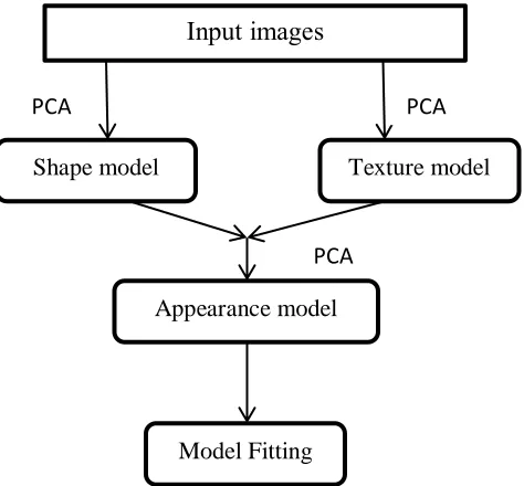
Mainly, AAM model can built in four parts: (i) A statistical shape model is built using a number of labelled training images; (ii) To model the variations of texture, a texture model is assembled which is represented by pixel intensity; (iii) An appearance model is built by combining the shape model and texture model [5]. (iv) Finally, the combined model is fitted with target image. Figure 1.2 explains the main parts of AAM.

Figure 1.2The basic parts of Active Appearance Model

.

Image Database

Feature Databas Feature

extraction (AAM)

Training data

Testing data

Classification PSO-SVMs

Result

Texture model Shape model

Appearance model

Model Fitting

Input images

PCA PCA

(3)

i. Statistical Shape Model

A shape model is constructed from a set of marked training images. A shape in 2-D case is characterized by concatenate vectors of n-point {(xi; yi)}

(

)

Then, the shapes that are constructed will be normalized by “Procrustes analysis process” [5] and projected on the shape subspace that is generated by “principle component analysis PCA”,

̅

where ̅ represents mean shape, Ps = {si} is a matrix contains a set of orthonormal base vectors si and drawing the modalities of variations that extracted from the training set, and made of shape variables in shape subspace. Thus, depends on the equivalent points, the images in training stage are warp to the mean shape to get “shape-free

patches”.

ii. Statistical Texture Model

The texture model is established more identically as the shape model. Depends on the shape model, the texture can be scanned into a vector g, and followed by process of linear normalization of texture, by the parameters

( ) and is given by

( )

,

where and are, correspondingly, represents mean and variance of the texture , and 1 = [1; 1, …..1] T is vector with the identical length of . Ultimately, depending on principle component analysis (PCA), texture is estimated on the texture subspace

̅

where ̅indicates to mean texture, { } represents matrix contains a set of orthonormal base vectors and defining modes of variation resulting from the training set, and comprises texture parameters of the texture subspace.

iii. Combined Appearance Model

In this stage, the joined relationship between the created shape and texture is examined by PCA and the appearance subspace is produced. The shape and the appearance can be labelled as follows:

̅

Where c represents vector of appearance parameters that control the shape and the texture together, and , are

(4)

Accordingly, the finishing appearance model can be characterized as b = Qc where:

(

) (

₍( _{) ( ̅)}) ( ̅)

)

and Q is representing the matrix of eigen vectors of b.

iv. Model Fitting

After creating the appearance model, it is significant to fit the created model with new images, which is vital to find the most suitable parameters of the model. However, this consider as an unconstrained optimization problem, which is more complex and challenging to solve. Usually, it can be addressed via “gradient descent algorithm”. Let p indicate the AAM parameters vector ( ) which is represents combination of the appearance parameters c, the texture transformation parameters u. and pose parameters t.

Besides, is represents the sampled texture vector of the current image, which is estimated to the texture model frame, and is represents the texture vector, produced via the model. There is a linear relationship between the texture difference between an image and the model and the variance of p which is given by:

( )

,

where, δp is a lesser variance of p, and R is represents the linear relationship (or gradient matrix) between δp and r. AAM assumes that R be fixed and computes it by multivariate linear regression methods. Since the relationship R is computed, fitting is an iterative procedure that can be carried out as follows (Gao et. al. 2010).

The texture of an image is sampled and projects it to texture model space.

Compute the residual texture vector, and assess the fitting correctness using | |2 , where | | mean the norm (2-norm generally).

Derived variance of parameters of the model by ( ). Update model parameters p → p + kδp, where k = 1 at first.

Through the new model parameters, compute the new model texture , and the texture, is resampled Compute the new residual vector, | | 2 .

If < E, then accept the update; if not, try at k = 0.5, 0.25, etc., at that time go to the first step.

These procedures repeat till there is no more enhancement.

1. Classification using PSO-SVM

“Support vector machine” (SVM) is supervised learning approach, which is very useful for classification and regression process [12]. Though, the selection process of the training parameters is influencing factor effects on the performance of SVM. SVM classifier is based on statistical learning theory, which is aimed at determining a hyperplane which efficiently separates two classes by using training dataset. Suppose that, a training dataset * + , where x is

(5)

Accordingly, determination of optimal hyperplane is essential for solve the optimization problem that given by:

‖ ‖

(

)

Figure 1.

3

The classification process of SVM.

The positive slack variables are presented to substitute the optimization problem, and the method could be extended to allow for nonlinear decision surfaces, the new optimization problem is given as:

‖ ‖

∑

(

)

Such that

∑

(

)

Where, is indicates to the penalty parameter or regularization constant. The penalty parameter controls the tradeoff between two competing criteria of error minimization and margin maximization. Therefore, the classification decision function can become:

( ) (∑

(

)

(6)

2. Parameters selection of SVM using PSO

“Particle swarm optimization” PSO mimics the swarm behavior of individuals which represent probable solutions in a

D-dimensional search space. Particle is contain four vectors:

( ) where represents its position in the dth dimension; ) where is the finest position in the dth dimension that particle has found on its own; ( ) , where indicate to the velocity in the dth dimension; and ) where is the global best position in the dth dimension for all particles. In the swarm, particles move over the search space as follows:

(

)

(

)

where is represents the inertia weight, and are velocity coefficients which come as a constants with the value of 2.0, and are random numbers with the range of [0.1] at each iteration from d=1 to D, is indicate to the velocity of the ith particle, is the present location of the particle , is represents the location of the finest fitness value of the particle at the present iteration and is represents the location of the particle with the finest fitness value in the swarm.

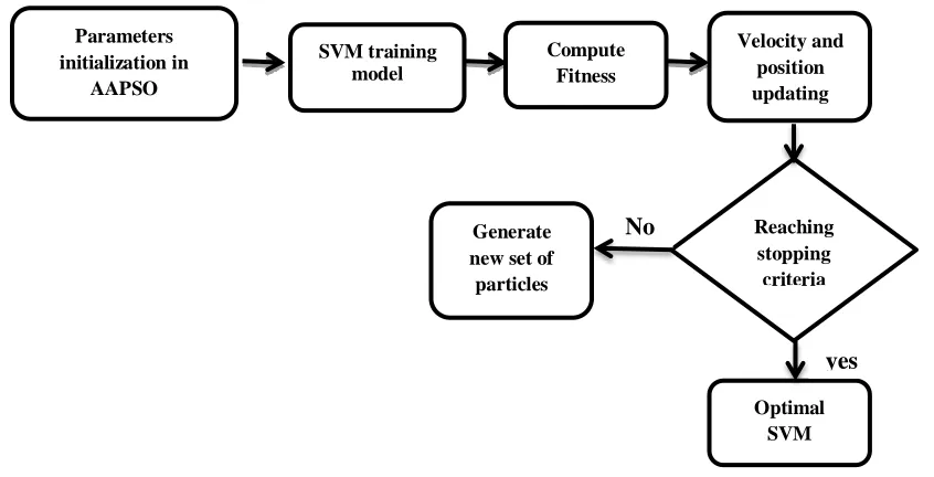
3. Parameters Optimization of SVM by PSO

The parameters of SVM are optimized by PSO procedure to attain a precise recognition result. The SVM optimization process by PSO is described in the figure as below:

Figure 1.4Parameter optimization of SVM using PSO.

Parameters initialization in

AAPSO

SVM training model

Compute Fitness

Velocity and position updating

Reaching stopping criteria Generate

new set of particles

Optimal SVM parameters No

(7)

3. EPERIMENTAL RESULTS

The proposed technique executed in the MATLAB platform. The proposed method is assessed with three face datasets YALE, CASIA and FERET under different lighting conditions. In our technique the face images are tested with two conditions as follows:

• Face images with same illumination

• Face images with different illumination

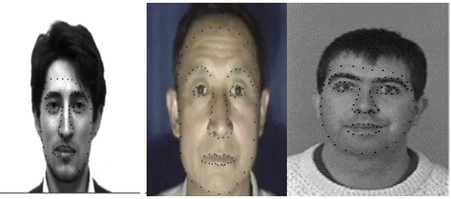
The three datasets are divided into training and testing datasets. In Yale dataset, there are 15 classes, in each class there are different images in different illumination conditions. In the experimental tests, 165 images have been used in the evaluation process 75 images for training and 90 images for testing. From CASIA database, 500 images have been used and have been separated to five datasets. In each dataset, there are 100 images at five illumination variations while FERET dataset, same thing as CASIA has been done for FERET dataset. Figure 1.3 shows examples of images for the three datasets. In the evaluation process, the images in each datasets have been equally divided for training and testing. In order to demonstrate the efficiency and the stability of the proposed method, the facial images have been assessed on two conditions: (i) identical pose with different illumination conditions (ii) identical pose with the same illumination. To achieve the performance analysis process, we have performed the different rounds of experiments by AAM+PSO-SVM method. The Table 1.1 and Figure 1.4 illustrate the accuracy of outcomes generated by the proposed face recognition method (AAM+PSO-SVM) against the existing OPSO-SVM and PSO-SVM face recognition approaches.

(8)

Table 1.1:Accuracy values of the proposed AAM+PSO-SVM technique with three datasets.

C o n d it i ons Condition description Yale Dataset FERET Dataset CASIA Dataset

1 identical pose with different

illumination conditions

Method Accuracy Method Accuracy Method Accuracy

PSO-SVM 80

PSO-SVM

88 PSO-SVM 75

OPSO-SVM 75

OPSO-SVM

82

OPSO-SVM

85

AAM+ OPSO-SVM

89 AAM+

OPSO-SVM

85 AAM+

OPSO-SVM

90

2 identical pose with the same illumination

conditions

PSO-SVM 84

PSO-SVM

90 PSO-SVM 88

OPSO-SVM 85

OPSO-SVM

85

OPSO-SVM

90

AAM+ OPSO-SVM

92 AAM+

OPSO-SVM

90 AAM+

OPSO-SVM

92

(a)

(b)

Figure 1.6Average accuracy performances of the proposed AAM+ PSO-SVM and PSO-SVM, OPSO-SVM methods

.

65 70 75 80 85 90 95

Yale FERET CASIA

A

cc

ur

acy

Identical pose with different illumination conditions PSO-SVM OPSO-SVM AAM+ OPSO-SVM 80 85 90 95

Yale FERET CASIA

A

cc

ur

acy

identical pose with the same illumination conditions PSO-SVM

OPSO-SVM

(9)

4. CONCLUSION

Face recognition technique had been introduced in this paper. The proposed technique was based on two stages which were active appearance model (AAM) and PSO-SVM methods. AAM has been used to extracts the face features and those features were given to the PSO-SVM method to classify them according to the correct face class. Three different datasets have been used in the experimental results with different illumination conditions: YALE, FERET and CASIA dataset respectively. The accuracy metric has been used for the evaluation purpose. The proposed technique was outperformed than the other face recognition techniques such as (OPSO-SVM) [8] and (PSO-SVM) [11] in terms of recognition accuracy especially with YALE and CASIA database. One problem arises when we fitted the AAM model with the original face model which is that the time which can be reduced in the future work.

REFERENCES

[1] Anil K. Jain and Ajay Kumar, "Biometrics of Next Generation: An Overview", Second Generation Biometrics, Springer, 2012 [2] Huang, Heisele and Blanz, “Component-based Face Recognition with 3D Morphable Models”, In Proceedings of the 4th International Conference on Audio-and Video-Based Biometric Person Authentication, AVBPA, Guildford, UK, pp. 27-34, 2003 [3] Patil, Kolhe and Patil, "2D Face Recognition Techniques: A Survey", International Journal of Machine Intelligence, Vol. 2, No. 1, pp-74-83, 2010

[4] Dinesh Govindaraj, "Application of Active Appearance Model to Automatic Face Replacement", Journal of Applied Statistics, 2011

[5] Cootes, T.F., Edwards, G. J. & Taylor, C. J.1998. Active appearance models. In Proc. Eur. Conf. Comput. Vis. 2, pp. 484–498 [6] M. H. Abdulameer, S. N. H. Sheikh Abdullah, and Z. A. Othman, “A Modified Active Appearance Model Based on an Adaptive Artificial Bee Colony,” The Scientific World Journal, vol. 2014, Article ID 879031, 16 pages, 2014.

[7] M. H. Abdulameer, S. N. H. Sheikh Abdullah, and Z. A. Othman, “Support vector machine based on adaptive acceleration particle swarm optimization,” The Scientific World Journal, vol.2014, Article ID 835607, 8 pages, 2014.

[8] M. H. Abdulameer, S. N. H. Sheikh Abdullah, and Z. A. Othman. 2013. “A Face Recognition system based on Opposition Particle Swarm Optimization (OPSO) and Support Vector machine (SVM),

[9] Weihong Li, Lijuan Liu and Weiguo Gong, “Multi-objective uniform design as a SVM model selection tool for face recognition”, Expert Systems with Applications, Vol. 38, No. 6, pp. 6689–6695, June 2011.

[10] Zhifeng Li and Xiaoou Tang, “Using Support Vector Machines to Enhance the Performance of Bayesian Face Recognition”, IEEE Transactions on Information Forensics and Security, Vol. 2, No. 2, pp. 174- 180, June 2007.

[11] Jin Wei, Zhang Jian-qi and Zhang Xiang, “Face recognition method based on support vector machine and particle swarm optimization”, Expert Systems with Applications, Vol. 38, No. 4, pp. 4390-4393, April, 2011