Article
1
A physically-constrained calibration database for
2
Land Surface Temperature using infrared retrieval
3
algorithms
4
João P. A. Martins 1,2, Isabel F. Trigo 1,2, Virgílio A. Bento 2 and Carlos da Camara 2,*
5
1 Instituto Português do Mar e da Atmosfera, Lisbon, Portugal; E-mails: [email protected] (J.P.M.),
6
[email protected] (I.T.)
7
2 Instituto Dom Luiz, University of Lisbon, IDL, Campo Grande, Ed C1, 1749-016 Lisbon, Portugal;
8
E-Mails: [email protected] (V.B.); [email protected] (C.C.)
9
* Correspondence: [email protected]; Tel.: +351 21 844 7055, Ext: 1555
10
11
12
Abstract: Land Surface Temperature (LST) is routinely retrieved from remote sensing
13
instruments using semi-empirical relationships between top of atmosphere (TOA) radiances and
14
LST, using ancillary data such as total column water vapor or emissivity. These algorithms are
15
calibrated using a set of forward radiative transfer simulations that return the TOA radiances given
16
the LST and the thermodynamic profiles. The simulations are done in order to cover a wide range of
17
surface and atmospheric conditions and viewing geometries. This work analyses calibration
18
strategies, considering some of the most critical factors that need to be taken into account when
19
building a calibration dataset, covering the full dynamic range of relevant variables. A sensitivity
20
analysis of split-windows and single channel algorithms revealed that selecting a set of atmospheric
21
profiles that spans the full range of surface temperatures and total column water vapor
22
combinations that are physically possible seems beneficial for the quality of the regression model.
23
However, the calibration is extremely sensitive to the low-level structure of the atmosphere
24
indicating that the presence of atmospheric boundary layer features such as temperature inversions
25
or strong vertical gradients of thermodynamic properties may affect LST retrievals in a non-trivial
26
way. This article describes the criteria established in the EUMETSAT Land Surface Analysis –
27
Satellite Application Facility to calibrate its LST algorithms applied both for current and forthcoming
28
sensors.
29
Keywords: Land Surface Temperature; Thermal Infrared; Calibration; Generalized Split-Window;
30
Mono-Window; Database; Radiative Transfer
31
32
33
1. Introduction
34
Land surface temperature (LST) is an important parameter in the physics of the Earth surface.
35
LST controls the surface emitted long-wave radiation and is thereby essential to quantify sensible
36
and latent heat fluxes between Earth surface and atmosphere. These interactions are crucial for a
37
variety of applications related to land surface processes, such as climate and drought monitoring
38
[1,2], hydrological cycle [3–5], model assessment [6–9], data assimilation [10–12], among others. LST
39
has been retrieved in remote sensing platforms using a variety of algorithms that rely on sensor
40
channels in the so-called atmospheric window region of the infrared spectrum [13]. Within this
41
band, surface emitted radiances reach the sensor with relatively little absorption by the atmosphere.
42
Moreover, in the thermal infrared atmospheric window (TIR), surface emissivity can be determined
43
with relatively less uncertainty than in other regions in the infrared, such as in the middle infrared,
44
the middle infrared for LST estimation [13,15,16], however, these are far less common than
46
algorithms based on the thermal infrared observations, and therefore will not be considered here.
47
The choice of LST algorithm, which is often a semi-empirical function of top-of-atmosphere
48
(TOA) brightness temperatures in TIR, is intrinsically linked to the characteristics of the sensor being
49
used. As such, LST algorithms may rely on a single channel (the mono-window algorithms, MW),
50
when measurements are available in only one TIR band [15,17–19], or in a combination of TIR
51
channels using the so-called generalized split-windows (GSW) approach [13,20,21]. In general, this
52
type of algorithms are based on a linear regression between the measured quantities at the top of the
53
atmosphere and LST, using ancillary data such as spectral emissivity, total column water vapor
54
(TCWV), zenith viewing angle (ZVA), land cover and also day / night flags. Usually these
55
parameters are divided into classes and for each combination a set of model coefficients is estimated
56
[13,20]. The whole procedure therefore requires setting up a comprehensive calibration database
57
which is usually ad hoc generated, with a high risk of leaving out unforeseen situations that lead to
58
systematic biases in operational retrievals. To the best of our knowledge, no study has been devoted
59
to the process of building a calibration database. This paper focus on the factors that need to be taken
60
into account when building a calibration database for such regressions, providing a general
61
methodology that can be applied when developing an algorithm for infrared LST estimates and
62
providing a systematic discussion of the impact of all the choices that are made when building a
63
calibration database.
64
In order to make the model coefficients robust enough to deal with any combination of input
65
parameters it is necessary to calibrate the model for a wide range of atmospheric and surface
66
conditions as well as viewing geometries. A good calibration of the model coefficients can only be
67
achieved if the calibration database is designed carefully, covering the range of variations that are
68
expected to affect the problem [21]. Usually, the models are calibrated using criteria that are
69
considered reasonable, covering a wide range of atmospheric and surface conditions [20,22], but
70
here we propose an objective approach to prepare a calibration database that minimizes the overall
71
model error statistics and their variations among the range of input parameters.
72
This article summarizes the procedure used in the EUMETSAT LSA SAF [23] to calibrate LST
73
algorithms for the Spinning Enhanced Visible and InfraRed Imager (SEVIRI, e.g. [20]) onboard the
74
Meteosat Second Generation (MSG), the Advanced Very-High Resolution Radiometer (AVHRR) on
75
Metop and the Meteosat Visible and InfraRed Imager (MVIRI) onboard Meteosat First Generation
76
(MFG; e.g., [17]). The current standard methodology within the LSA SAF uses a criteria for setting
77
up the calibration database with a good compromise addressing the widest possible retrieval
78
conditions (which is a pre-requisite for a global LST product) but a sensitivity analysis was required
79
to ensure that the most robust possible model coefficients are in use. A similar exercise will be soon
80
performed for the Flexible Combined Imager (FCI) on board Meteosat Third Generation (MTG; [24])
81
to design the follow-on of LSA SAF operational LST products.
82
2. Methodology
83
2.1 The problem
84
Considering the Earth surface as a lambertian emitter-reflector, a cloud-free atmosphere under
85
local thermodynamic equilibrium and negligible atmospheric scattering, the monochromatic top of
86
atmosphere radiance 𝐿𝑖, in a given channel i, and measured by a sensor onboard a satellite
87
observing the Earth’s surface under zenith angle θ is expressed by (e.g. [13]):
88
𝐿
𝑖(θ) = 𝐵(𝑇
𝑏𝑖) = 𝜖
𝑖𝐵
𝑖�𝑇
𝑠𝑠𝑠�𝜏
𝑖(𝜃) + 𝐿
↑𝑎𝑎𝑎,𝑖(𝜃) + (1 − 𝜖
𝑖)𝐿
↓𝑎𝑎𝑎,𝑖𝜏
𝑖(𝜃),
(1)
where 𝜖𝑖 is the surface emissivity on channel i, 𝐵𝑖(𝑇𝑠𝑠𝑠) is the equivalent black-body radiance at
89
temperature 𝑇𝑠𝑠𝑠 (or LST), 𝜏𝑖 is the transmissivity, 𝐿𝑎𝑎𝑎,𝑖↑ is the upward atmosphere-emitted
90
radiance, and 𝐿𝑎𝑎𝑎,𝑖↓ is the downward atmosphere-emitted radiance. LST is often estimated from
91
There are a few formulations of these inversions in the literature [25] which mostly depend on how
93
the Taylor expansion of the radiative transfer equation is made in order to derive a formulation that
94
is suitable to a particular application. In this work the sensitivity to the used model is not fully
95
addressed, although some of the results could be slightly different if different LST algorithms were
96
used. However, it is important to assess the differences of using a GSW model or a MW model, as
97
they serve two different purposes: the first is widely used in state of the art retrieval schemes in
98
sensors with two or more channels in the thermal atmospheric window, while the second is left for
99
sensors with only one channel in that band. Here, only one formulation for each case is considered –
100
one GSW and one MW algorithm – which will serve as testbeds for the calibration datasets under
101
analysis. The GSW formulation used for operational LST estimates both from the Moderate
102
Resolution Imaging Spectroradiometer (MODIS; [21]) and from SEVIRI ([20]):
103
𝐿𝐿𝑇 = 𝐶 + �𝐴1+ 𝐴21 − 𝜖𝜖 + 𝐴3Δ𝜖𝜖2�𝑇𝐼𝐼1+ 𝑇2 𝐼𝐼2
+ �𝐵1+ 𝐵21 − 𝜖𝜖 + 𝐵3Δ𝜖𝜖2�𝑇𝐼𝐼1− 𝑇2 𝐼𝐼2
,
(2)
where 𝐴1,𝐴2, 𝐴3,𝐵1, 𝐵2, 𝐵3 and 𝐶 are the model coefficients, 𝑇𝐼𝐼1 and 𝑇𝐼𝐼2 are the equivalent
104
brightness temperatures, 𝜖 and Δ𝜖 are the average and the difference of the emissivities in both
105
split-windows channels. For the MW model, the formulation derived by Duguay-Tetzlaff et al. [17]
106
to derive LST from Meteosat First Generation is used:
107
𝐿𝐿𝑇 = 𝐴
𝑇𝐼𝐼1𝜖𝐼𝐼1
+ 𝐵
1
𝜖𝐼𝐼1
+ 𝐶
,
(3)where again 𝐴, 𝐵, and 𝐶 are the regression coefficients. In both cases, the regression coefficients are
108
fit for classes of TCWV and ZVA, and they must somehow simulate atmospheric absorption and
109
emission, while the effect of surface emissivity is in these cases, explicitly resolved. The atmospheric
110
transmissivity is mainly constrained by the radiative optical path. Hence, a good calibration
111
database to fit model coefficients in eqs. (2) and (3) needs to ensure that a scene may be observed by
112
a wide range of viewing geometries (ZVA) and water vapor contents, which is the most relevant and
113
variable absorber/emitter in the TIR window region.
114
The weighting functions (given by the vertical derivative of transmissivity) of atmospheric
115
window channels peak close to the surface, where the strongest vertical gradients of humidity are.
116
However, in the presence of well-developed moist planetary boundary layers their peak will be
117
higher above (although always relatively close to the ground), which means the temperature and
118
humidity vertical structure at the lower levels in the profiles represented in the calibration database
119
might play a role in the database robustness, especially considering the occurrence of temperature
120
inversions close to the surface. This effect may be taken into account not only by introducing a large
121
variety of atmospheric profiles at different locations and observation times, but also by artificially
122
varying the difference between the surface skin temperature and the near-surface air temperature
123
(𝐿𝐿𝑇 − 𝑇𝑎𝑖𝑎), which in turn has a significant role in the control of the thermal structure of the lower
124
atmosphere, through the turbulent sensible heat flux (e.g., [26,27]). This difference varies across the
125
diurnal cycle, among surface types and for different large scale atmospheric conditions, and may be
126
either positive or negative. Particular attention should be paid to its distribution within calibration
127
databases and to the impact on algorithm performance.
128
The difference between TOA brightness temperatures in the split-window channels is aimed at
129
capturing differential absorption within those bands which is associated to atmospheric water vapor
130
content. In the case of a GSW algorithm, eq (3), the difference between the spectral emissivities of the
131
window channels are also taken into account. This difference is related to surface type and moisture
132
in the sense that moister surfaces show less spectral variations in emissivity [28].
133
The development of LST algorithms, such as those represented by eqs. (2) and (3) (see e.g.,
135
[20,21,25]) is usually based on a set of radiative transfer simulations performed for a calibration
136
database (for algorithm fit) and a validation one (for algorithm test), both representing a wide range
137
of clear sky conditions. The databases must be independent and, while the former should
138
encapsulate the widest possible atmospheric conditions for the area of interest together with broad
139
distributions of surface emissivity and sensor viewing geometry that are needed for robust
140
parameter estimation, the latter should contain the largest possible set of profiles/surface conditions
141
to allow a comprehensive characterization of LST algorithm uncertainty. By LST algorithm
142
uncertainty, we mean deviations of LST retrievals from the “true value” that are not associated to
143
uncertainties in the input data, but solely to the retrieval method. The characterization of the
144
individual sources of uncertainty (such as the algorithm uncertainty studied here or the uncertainty
145
due to emissivity or to the sensor noise, for example) has been recognized as crucial for the
146
uncertainty validation of remotely sensed surface temperature products [29]. It is worth
147
emphasizing that the comparison of LST estimates obtained using actual remote sensing
148
observations against ground-based observations is part of a product validation exercise. In that case,
149
which is often limited to a relatively small number of available sites, the deviations will be the result
150
of both algorithm and input errors and their contributions to the total error are impossible to
151
disentangle. The radiative transfer simulations aim to determine the TOA spectral radiances for each
152
profile in the respective databases, so that the forward problem is solved with full knowledge of the
153
surface emission and atmospheric absorption. It is important that those simulations are performed
154
with an accurate radiative transfer model. For the example analyzed in this study, the MODTRAN4
155
code [30] was used, which returns spectral radiances with a resolution of 1 cm-1. For the sake of
156
simplicity, MODTRAN4 TOA radiances were convoluted with SEVIRI response functions for
157
channels centered at 10.8 µm (IR1 channel) and 12.0 µm (IR2 channel, only used in the GSW
158
algorithm), and then subject to the inverse Planck function to obtain the respective channels
159
brightness temperatures, 𝑇𝐼𝐼1 and 𝑇𝐼𝐼2 (for more details see, e.g. [15]). The calibration of the
160
coefficients is performed using a least-squares technique, aimed to provide the best fit for the
161
semi-empirical relationships between the simulated brightness temperatures and the set of
162
prescribed LSTs, atmospheric conditions and viewing geometries in the calibration database. In the
163
case of eqs. (2) and (3) used in this study, the coefficients are calibrated in classes of ZVA and TCWV,
164
as those formulations do not explicitly model their effect on the atmospheric correction. Finally, the
165
algorithm uncertainty is characterized using the independent validation database, through
166
comparisons of estimated LST obtained with one of the semi-empirical models (eq. 2 or 3) and the
167
𝐿𝐿𝑇𝑇𝑎𝑇𝑇 value. The latter corresponds to the 𝑇𝑆𝑆𝑖𝑆 values in the databases, which together with the
168
respective atmospheric profiles, surface emissivity and prescribed view zenith angle, led to the TOA
169
brightness temperature(s) used in the LST algorithms. The use of independent databases for
170
algorithm calibration and validation, relying on accurate radiative transfer simulations, is the best
171
way of characterizing the algorithm uncertainty and its performance for a wide range of scenarios.
172
2.3 Characteristics of Atmospheric Profiles relevant for Radiative Transfer in the TIR Window
173
We have opted to select the calibration dataset from a comprehensive collection of clear-sky
174
profiles of temperature, water vapor and ozone, as well as ancillary variables such as spectral
175
emissivity, land cover, elevation, skin temperature, and surface pressure compiled by Borbas et al.
176
[31]. This dataset, hereafter referred to as SeeBor database, includes over 15000 profiles and will be
177
used in this work for convenience. We could have made use of other datasets also specifically
178
gathered for satellite retrievals under clear sky conditions (e.g., [22]), however our aim is focused on
179
the criteria to be taken into account for the subset of calibration data for LST algorithms.
180
Figure 1 shows the geographical distribution of profiles contained in the SeeBor database; the
181
dots representing the profile locations are colored according to their TCWV. This dataset covers the
182
whole globe, including oceans. Regions with more frequent cloud cover are, as expected, somewhat
183
less populated. In general, low values of TCWV are found near the poles and high values close to the
184
possible to observe both very dry and very moist atmospheres. From this large set of profiles only a
186
few will be selected to calibrate an LST retrieval algorithm, while the rest is used for its validation,
187
i.e., characterization of algorithm uncertainty as referred above. The task of selecting these
188
calibration profiles is tricky and impacts on the model robustness, as will be shown below.
189
190
Figure 1 - Distribution of the SeeBor (clear sky) profiles, colored by TCWV class (in cm).
191
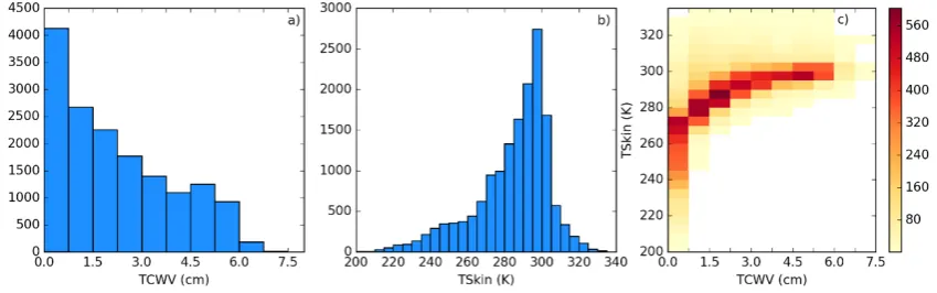
The statistical distributions of TCWV and skin temperature are shown in Figure 2a and 2b,
192
respectively. Both distributions are highly skewed. The majority of the profiles are on the drier side
193
of the TCWV distribution and almost no profiles show values of more than 6 cm since those
194
conditions are within the physical limit for an atmosphere with no clouds. Skin temperatures show a
195
wide dynamic range, roughly between 210 and 330 K, the distribution being negatively skewed. So
196
in principle, it would only be necessary to uniformly span these ranges of values to have a
197
comprehensive calibration database. However, some combinations of both parameters are
198
unphysical, which in turn leads to less accurate coefficients and a less performant regression model.
199
The bivariate distribution shown in Figure 2c reveals that not surprisingly very moist (clear sky)
200
atmospheres only occur over the warmer surfaces, while towards lower TCWV values, the skin
201
temperature range increases. In other words, the very dry atmospheres can be very warm or very
202
cold, whereas the moister atmospheres are only found over warmer surfaces.
203
204
Figure 2 - Distributions of a) TCWV and b) Skin temperature on the SeeBor database. c) Bivariate
205
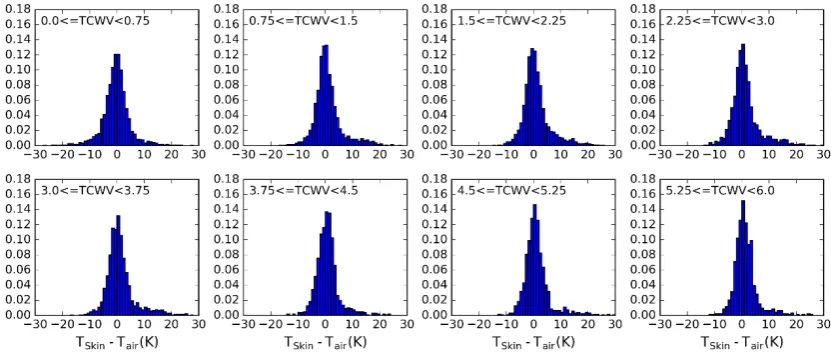
In Figure 3 the distribution of 𝐿𝐿𝑇 − 𝑇𝑎𝑖𝑎 is shown, for each class of TCWV. 𝑇𝑎𝑖𝑎 corresponds
207
to the temperature at the first pressure level above the ground. The separation in classes of TCWV
208
shows that drier atmospheres support somewhat larger temperature gradients close to the surface.
209
The dynamic range of this parameter needs to be chosen carefully, since it has a large impact on the
210
resulting coefficients (see sensitivity tests in section 3). Cases with the largest differences should also
211
be accounted for in the linear regression, otherwise the calibration would miss some of the most
212
extreme low level temperature profiles and this would degrade the quality of the regression,
213
especially when the algorithm needs to deal with such profiles in practice. For very dry
214
atmospheres, the distribution is nearly normal with maximum absolute differences of about 20 K. In
215
the case of moister atmospheres, the distributions become positively skewed with maximum
216
positive differences of about 25 K for only a few cases but almost no values below -10 K. In general,
217
most cases lie between -15K and 15K.
218
219
Figure 3 - Distributions of the difference between the skin temperature and the temperature at the
220
first level above the surface on SeeBor, by class of TCWV. Histograms are normalized by the number
221
of cases in each TCWV class.
222
The diversity of land surfaces and the radiative properties of their materials need to be taken
223
into account through an appropriate range of surface emissivities. This quantity adds an extra level
224
of complexity to the calibration database. Depending on the algorithm that is chosen, only one value
225
is used in the case of a single-channel algorithm, or the values on two bands need to be specified in
226
the case of a GSW model. Some GSWs, such as that considered here (eq. 2) rely on the average value
227
of the emissivity in the two channels and also the difference between them. Therefore it was decided
228
to prescribe a range of emissivity values for the channel around 10.8 µm and then prescribe a range
229
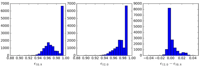
of differences of the emissivities in both channels, 𝛥𝜖 = 𝜖𝐼𝐼2− 𝜖𝐼𝐼1. The range of spectral emissivities
230
at 10.8 µm and 12.0 µm, close to typical central wavelengths of split-window channels (e.g., MODIS,
231
SEVIRI), available in the SeeBor database are shown in Figure 4. There are quite a few cases with
232
very high emissivities which correspond to SeeBor profiles over water bodies and ice. In general,
233
cases over land have higher emissivities in the 12.0 µm compared to the 10.8 µm. The larger spectral
234
variations are found over deserts and semi-arid surfaces.
235
The viewing angle also affects the calibration and the appropriate range to be considered will
236
depend on each sensor. In this work the analysis will be for a sensor on board a geostationary
237
platform, or for a large swath polar orbiting sensor, and therefore we will also consider a wide range
238
240
Figure 4 – Distribution of the SeeBor spectral emissivities at 10.8 and 12.0 µm, and their difference.
241
2.4 A calibration database
242
Given the physical constraints of the problem and the range of the input parameters detailed in
243
the previous section, the following methodology is proposed to select the subset of calibration
244
profiles:
245
1) Define classes of 𝑇𝑆𝑆𝑖𝑆 (from 200 K to 330 K in steps of 5 K) and 𝑇𝐶𝑇𝑇 (from 0 to 6 cm in
246
classes of 0.75 cm – values greater than this should be treated with the coefficient
247
corresponding to the last 𝑇𝐶𝑇𝑇 class).
248
2) Iterate in the SeeBor clear-sky profile database to fill each class in the 𝑇𝐶𝑇𝑇/ 𝑇𝑆𝑆𝑖𝑆 phase
249
space (as in Figure 2c) with one case each. When a new profile is selected, it is ensured that
250
its great-circle distance to the already selected profiles is greater than an initial distance of 15
251
degrees, which guarantees a wide geographical coverage. After a sufficiently large number
252
of tries (in this case 30000), the distance criterion is relaxed in steps of minus 1 degree, until
253
the whole 𝑇𝐶𝑇𝑇/ 𝑇𝑆𝑆𝑖𝑆 phase space is filled.
254
3) For each of the previously selected profiles, assign a new 𝑇𝑆𝑆𝑖𝑆 based on the ranges of
255
𝑇𝑆𝑆𝑖𝑆− 𝑇𝑎𝑖𝑎 observed in Figure 3. The choice of the range of perturbations to apply is key to
256
the performance of the chosen model and may depend on the region of interest. In the case
257
of this work, a range of ±15K around 𝑇𝑎𝑖𝑎 in steps of 5K showed an overall good
258
performance. As will be seen, large biases arise when non-physical cases are included or if
259
the somewhat more extreme cases are not taken into account.
260
4) Each of these conditions may be sensed from angles ranging from 0 (nadir view) to 70° in
261
steps of 2.5°. It is important to discretize the viewing geometry in this way because this is an
262
intrinsically non-linear problem. The upper limit of the 𝑍𝑇𝐴 might be adapted for the
263
sensor under analysis. Previous calibration exercises show that above this viewing angle
264
limit the retrieval errors are generally too high, especially for moister atmospheres [15].
265
5) For the emissivity, a range of possible values are attributed to each of the cases above: values
266
of 𝜖10.8 from 0.93 to 1.0 in steps of 0.01 and then, in the case of a GSW model, it is
267
appropriate to prescribe departures from this value for 𝜖12.0: -0.015 to 0.035 in steps of 0.01
268
(excluding cases where 𝜖12.0> 1.0), as suggested by Figure 4.
269
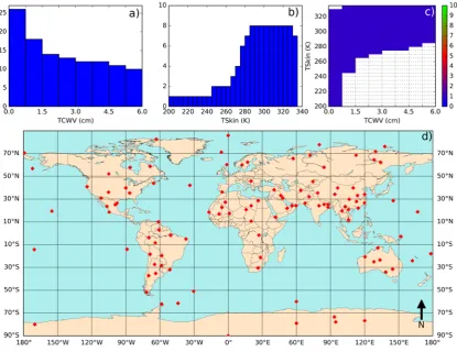
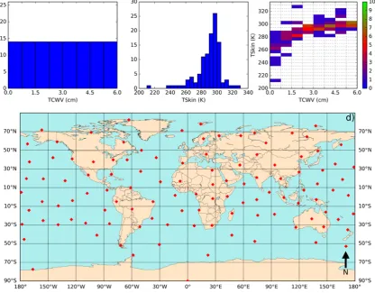
Figure 5 shows the statistical and geographical properties of the database gathered following
270
those steps, which total 116 profiles. By combining these profiles with the prescribed viewing
271
geometries and surface / low-level conditions proposed in steps 3 to 5, the total number of cases used
272
in the calibration is 906192. This number is around ten times larger than the number of simulations
273
made for the validation dataset, which contains the remaining profiles in the SeeBor database,
274
simulated with five random angles (within the ZVA range of each sensor) per profile. Note that the
275
TCWV distribution (Fig. 5a) is close to that of the whole SeeBor data set (Fig. 2a), although moister
276
profiles are relatively over-represented, so that a robust fit of LST algorithms can be achieved for
277
these cases. Nevertheless, low humidity profiles still dominate within the distribution, to ensure a
278
proper coverage of the 𝑇𝐶𝑇𝑇/ 𝑇𝑆𝑆𝑖𝑆 phase space (Fig. 5c) and its large dynamic range of 𝑇𝑆𝑆𝑖𝑆
279
The way the database is built also leads to a larger frequency of profiles gathered over land,
281
since some of the most extreme conditions are only found there. The presence of some marine
282
profiles is not problematic because algorithms also need to cover cases where the LST retrieval is
283
made over small islands or coastal regions. Validation of LST products over large water bodies is
284
also a common practice (e.g. [32]).
285
286
Figure 5 – Main properties of the proposed calibration database: a) TCWV distribution, b) 𝑇𝑆𝑆𝑖𝑆
287
distribution, c) Bivariate TCWV/𝑇𝑆𝑆𝑖𝑆 distribution and d) geographical distribution.
288
3. Results
289
3.1 Error statistics of the proposed calibration database
290
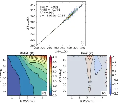
Figure 6 shows the error statistics of the GSW algorithm adjusted using the proposed calibration
291
database; the algorithm error (i.e., LSTGSW – LSTTrue) statistics are evaluated for the independent
292
validation database. Globally, this reveals a bias of around -0.09 K and a Root Mean Square Error
293
(RMSE) of 0.776 K, the scatterplot shows larger dispersions towards larger LSTs which is mainly
294
caused by the greater water vapor content of such atmospheres. Especially when combined with
295
large viewing angles, this kind of profiles is responsible for the largest retrieval errors. This is
296
confirmed by the diagram on the center of Figure 6 which shows the RMSE per class of VZA and
297
TCWV: larger RMSE values of above 3 K appear for classes with larger optical path (larger ZVA and
298
larger TCWV). On the other hand, nearly all classes below 3 cm and below 50 degrees show RMSEs
299
of 0.5 K or lower. The distribution of the bias over the TCWV/ZVA diagram shows that this statistic
300
does not change much across the different classes with only a few classes with positive and negative
301
303
Figure 6 - Error statistics for the proposed calibration database using the GSW model. On the left a
304
scatterplot with all the cases in the database, and the global bias and RMSE are indicated. The red
305
line represents the best linear fit. On the center, the RMSE is calculated for boxes of TCWV and VZA
306
and on the right the same is done for the bias.
307
In Figure 7 the same statistics are analyzed in the case of the MW model. Although this model
308
shows nearly the same overall bias (0.086 K), its RMSE is almost three times larger (of about 2.20K).
309
The way the RMSE is distributed along the classes of TCWV and ZVA is much less linear than in the
310
case of the GSW model and presents a stronger dependency on TCWV even for low ZVAs. Moreover
311
there are more classes with retrieval errors that are close to the limit acceptable for LST algorithms
312
(e.g., LSA-SAF LST products consider 4K to be their threshold accuracy requirement; [20]). The bias
313
also has a more complex structure among the TCWV/ZVA classes, some of them reaching more than
314
1K, both positive and negative showing that the overall bias results from the cancellation of values
315
between different classes. The differences between Figure 6 and Figure 7 and particular the steeper
316
increase in RMSE with TCWV in the MW, emphasize the importance of using GSW-type schemes
317
319
Figure 7 - Same as Figure 6 but for the MW model.
320
3.2 Sensitivity to the distribution of relevant variables
321
In order to study the sensitivity of the proposed database to some of the choices that were
322
made, a set of experiments was performed. The baseline calibration dataset, which is based on a
323
choice of profiles that is adequate to fill the TCWV/LST diagram is referred to as WTS_-15_15
324
(TCWV is sometimes represented as W in the literature and TS stands for 𝑇𝑆𝑆𝑖𝑆). A different criterion
325
could have been adopted to choose a few calibration profiles from the more than 15000 profiles in
326
the SeeBor database, such as ensuring a flat distribution of TCWV. This criterion was adopted,
327
together the wide geographical distribution criterion of WTS_-15_15, for experiments
328
FLAT14_-15_15 and FLAT10_-15_15. The difference between these two is that for the first, 14 profiles
329
per TCWV class were chosen (112 profiles vs. 116 in WTS_-15_15) and for the latter only 10 (leading
330
to a total of 80 profiles). The goal was to test the relevance of the number of profiles and of the
331
respective joint LST /TCWV distribution for the robustness of the regression coefficients. The
332
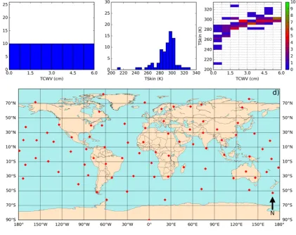
statistical and geographical distributions of these databases are illustrated in Figures 8 and 9. Large
333
parts of the TCWV/LST diagram are not covered such as the most extreme LST classes. In the
334
intermediate TCWV classes, a large number of the cases fall in the same LST range, as these
335
combinations are globally more frequent for clear sky conditions, and therefore also more frequent
336
in the SeeBor database. Note that a few of the profiles are common to FLAT14_-15_15 and to
337
FLAT10_-15_15; this is because the algorithm is initiated with the same random seed, which
338
generated the same random number sequence for all the experiments. The geographical
339
distributions show that relatively fewer profiles over land are selected, which might be explained by
340
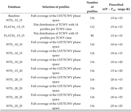
Table 1 – Description of the calibration database sensitivity experiments
342
Database Selection of profiles
Number of profiles
Prescribed
𝑳𝑳𝑳 − 𝑳𝒂𝒂𝒂 range (K)
Baseline: WTS_-15_15
Full coverage of the LST/TCWV phase
space 116 -15 to +15
FLAT14_-15_15 Flat distribution of TCWV with 14
profiles per TCWV class 112 -15 to +15
FLAT10_-15_15 Flat distribution of TCWV with 10
profiles per TCWV class 80 -15 to +15
WTS_-10_10 Full coverage of the LST/TCWV phase
space 116 -10 to +10
WTS_-10_15 Full coverage of the LST/TCWV phase
space 116 -10 to +15
WTS_-10_20 Full coverage of the LST/TCWV phase
space 116 -10 to +20
WTS_-15_20 Full coverage of the LST/TCWV phase
space 116 -15 to +20
WTS_-20_15 Full coverage of the LST/TCWV phase
space 116 -20 to +15
WTS_-20_20 Full coverage of the LST/TCWV phase
space 116 -20 to +20
WTS_-20_25 Full coverage of the LST/TCWV phase
space 116 -20 to +25
WTS_-25_25 Full coverage of the LST/TCWV phase
space 116 -25 to +25
343
Another factor that largely influences the robustness of the coefficients is the 𝐿𝐿𝑇 − 𝑇𝑎𝑖𝑎
344
difference. Therefore, we tested a few variants of the WTS_-15_15 database varying the lower and
345
upper limits of the prescribed 𝐿𝐿𝑇 − 𝑇𝑎𝑖𝑎 difference, always using steps of 5 K. These experiments
346
are referred to as WTS_-10_10, WTS_-10_15, WTS_-10_20, WTS_-15_20, WTS_-20_15, WTS_-20_20,
347
WTS_-20_25 and WTS_-25_25 (the numbers in the experiment name refer to the lower and upper
348
limits of 𝐿𝐿𝑇 − 𝑇𝑎𝑖𝑎). All these choices of calibration databases were tested in both the GSW and the
349
351
Figure 8 - Same as Figure 5 but for the FLAT14_-15_15 experiment.
352
The results of the sensitivity experiments are summarized in Table 1: the GSW and MW
353
algorithms were adjusted using the different calibration databases described above and assessed
354
using a common and independent validation database. In Table 1, values of the overall bias and
355
RMSE are indicated, as well as their variability among the TCWV/ZVA classes (via the standard
356
deviation of the bias and RMSE, respectively, obtained per TCWV/ZVA class). The GSW model
357
shows a slightly higher bias and RMSE using the FLAT approach when compared to the WPS. Their
358
variabilities are also larger for the FLAT-type databases, which means that there are classes that are
359
not so well represented when using this approach.
360
The set of experiments summarized in Table 1 also suggest high sensitivity to the lower and
361
upper limits of the prescribed 𝐿𝐿𝑇 − 𝑇𝑎𝑖𝑎 difference prescribed in the calibration databases as this
362
range is the only condition changing among experiments denoted by “WTS”. The results presented
363
in Table 1 suggest that it is hard to tell which combination is the best. In general, widening the
364
𝐿𝐿𝑇 − 𝑇𝑎𝑖𝑎 range of possible values seems to make the overall RMSE worse, although there are a few
365
exceptions. Another discernible pattern regards the sign and magnitude of the overall bias:
366
increasing the upper limit increases the bias (i.e. it becomes “more positive”); conversely, decreases
367
in the lower limit seem to make the bias more negative. Well balanced ranges (absolute value of the
368
370
Figure 9 - Same as Figure 5 but for FLAT10_-15_15.
371
Table 2 - Error statistics for the sensitivity experiments. The bias is calculated averaging the
372
difference 𝐿𝐿𝑇𝐺𝑆𝐺− 𝐿𝐿𝑇𝑇𝑎𝑇𝑇 for the validation database. The database with the best statistic is
373
highlighted in red.
374
Database Bias (K) RMSE (K) Bias stdev (K) RMSE stdev
(K)
Baseline: WTS_-15_15 -0.09 0.78 0.14 0.67
FLAT14_-15_15 -0.12 0.81 0.38 0.70
FLAT10_-15_15 -0.11 0.82 0.32 0.72
WTS_-10_10 0.05 0.74 0.26 0.64
WTS_-10_15 0.07 0.76 0.34 0.69
WTS_-10_20 0.09 0.81 0.41 0.73
WTS_-15_20 -0.02 0.76 0.21 0.67
WTS_-20_15 -0.11 0.79 0.14 0.68
WTS_-20_20 -0.12 0.78 0.14 0.68
WTS_-20_25 -0.11 0.78 0.15 0.68
WTS_-25_25 -0.25 0.87 0.22 0.73
375
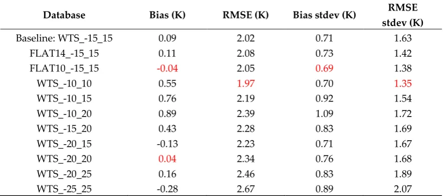
In the case of the MW model, the experiments show even less linear results. In fact, the case
376
with more favorable error statistics is arguably FLAT10_-15_15, with a lower absolute value of the
377
bias and bias variability, an overall RMSE that is comparable to that of the baseline experiment and
378
with less variability among classes. For the MW model, the experiment with the smallest RMSE is
379
the case of the GSW model, there is also a tendency to get worse RMSE values towards wider ranges
381
of 𝐿𝐿𝑇 − 𝑇𝑎𝑖𝑎 difference.
382
Table 3 – Same as Table 2 but for the MW model.
383
Database Bias (K) RMSE (K) Bias stdev (K) RMSE
stdev (K)
Baseline: WTS_-15_15 0.09 2.02 0.71 1.63
FLAT14_-15_15 0.11 2.08 0.73 1.42
FLAT10_-15_15 -0.04 2.05 0.69 1.38
WTS_-10_10 0.55 1.97 0.70 1.35
WTS_-10_15 0.76 2.19 0.92 1.54
WTS_-10_20 0.89 2.39 1.09 1.72
WTS_-15_20 0.43 2.28 0.83 1.69
WTS_-20_15 -0.13 2.23 0.71 1.67
WTS_-20_20 0.04 2.34 0.76 1.68
WTS_-20_25 0.16 2.46 0.83 1.89
WTS_-25_25 -0.28 2.67 0.89 2.07
384
These results suggest that the configuration of an appropriate calibration database may vary
385
with the algorithm to be used and area coverage, as the distribution of the variables analyzed above
386
(most notably 𝐿𝐿𝑇 − 𝑇𝑎𝑖𝑎) over the area of interest may support the exclusion of more extreme cases
387
and non-relevant. The choice of profiles from a SeeBor-like database is non-trivial but basing the
388
choice on fully covering the bivariate TCWV/LST distribution over the respective region of interest
389
seems to show some advantages. It is worth noticing that covering the most frequent classes in the
390
TCWV/LST diagram leads, as expected, to better overall statistics, as those will be the most frequent
391
in the validation database (and also in real applications). In Figure 10 the overall statistics are
392
analyzed for the FLAT14_-15_15 calibration database, which despite having a comparable number of
393
profiles to WTS_-15_15 and much more than FLAT10_-15_15, shows overall worse performance than
394
those cases. The analysis of the bias (Figure 10c) as a function of TCWV clearly shows that some
395
classes are affected by large negative biases (between 2 and 3 cm, and around 5 cm) while between 3
396
and 4 cm the bias is positive; the ZVA dependency seems less important in the analyzed case. This
397
shows that even with a flat distribution of TCWV, the performance of the model will depend on the
398
TCWV, suggesting that combined distributions of variables relevant to the problem need to be taken
399
into account. In practice this would translate in a roughly latitude dependent bias (following the
400
402
Figure 10 - Same as Figure 7 but using the FLAT14_-15_15 calibration database.
403
In order to explore the effect of the prescribed 𝐿𝐿𝑇 − 𝑇𝑎𝑖𝑎 differences in the representation of
404
the most extreme cases, boxplots of the error distribution (as given by 𝐿𝐿𝑇𝑀𝐺− 𝐿𝐿𝑇𝑇𝑎𝑇𝑇) were
405
calculated by classes of 𝐿𝐿𝑇 − 𝑇𝑎𝑖𝑎 in the validation database, and also as a function of the TCWV
406
class, for two of the proposed experiments: MW calibrated using WTS_-15_15 and WTS_-25_25,
407
respectively, as shown in Figures 11 and 12. There were some classes with only few cases, reflecting
408
the fact that largely negative differences rarely occur and they do so in very dry atmospheres,
409
therefore we merged them into a single class −25𝐾 ≤ 𝐿𝐿𝑇 − 𝑇𝑎𝑖𝑎< 10𝐾 to increase the figure
410
readability. Large positive differences are more frequent and may occur in all types of atmospheres.
411
The comparison of the error distributions shown in Figures 11 and 12 indicates that only a few
412
classes seem to be statistically affected by the temperature difference range that is applied. In drier
413
atmospheres (TCWV < 3cm) the effect is in fact negligible, since under these conditions the TOA
414
brightness temperatures will be highly dominated by the surface emitted signal (i.e., by LST and
415
surface emissivity). In most cases, the only noticeable effect is the increase in the range of the error
416
when the temperature difference increases, even in those classes that are “covered” by both
417
calibration databases (e.g., 5𝐾 ≤ 𝐿𝐿𝑇 − 𝑇𝑎𝑖𝑎< 10𝐾). This is what causes the overall loss of
418
performance of the database with the wider temperature ranges, since those classes are more
419
populated than those with more extreme temperature differences. It is also worth noticing that
420
extending the temperature difference range does not necessarily lead to a better representation of the
421
extreme cases. When 𝐿𝐿𝑇 − 𝑇𝑎𝑖𝑎 is positive and large, it likely means the surface sensible heat flux
422
may generate a convective boundary layer, which is often topped by a temperature inversion [33]. It
423
is well known that large LST retrieval errors occur under very moist atmospheres (e.g., [20]). If on
424
largest thermal and moisture gradients may be shifted upwards and therefore the peak of thermal
426
weighting function of (split-)window channels may also be shifted upwards [34–36], which makes it
427
harder to disentangle surface emission (LST and emissivity) from the signal emitted by the lower
428
atmosphere. Some currently used schemes address this issue using different coefficients for day and
429
night retrievals [e.g., 35], which somehow tunes the LST algorithms to different structures of the
430
atmospheric boundary layer, but introduce an additional discontinuity in the algorithm coefficients,
431
while other schemes use additional information from numerical weather prediction models
432
regarding near surface air temperature (which may also bring additional model forecast errors into
433
the retrieval). Although not shown, the GSW model seems much less sensitive to these effects, as the
434
boxplot diagrams for the cases illustrated in Figures 11 and 12 for the MW algorithm are much closer
435
to each other in the GSW case. In summary, extending the 𝐿𝐿𝑇 − 𝑇𝑎𝑖𝑎 values to include the most
436
extreme cases may not be beneficial for the overall performance of the retrievals because it can lead
437
to higher errors in the classes that are more frequent, without significant compensation from the
438
classes with more extreme situations.
439
440
441
Figure 11 - Boxplot diagrams of the 𝐿𝐿𝑇𝑀𝐺− 𝐿𝐿𝑇𝑇𝑎𝑇𝑇 difference (K) discriminated in classes of
442
𝐿𝐿𝑇 − 𝑇𝑎𝑖𝑎 difference (K) and TCWV, using the WTS_-15_15 database. Below each diagram the
443
number of cases is indicated. Note that the 𝐿𝐿𝑇 − 𝑇𝑎𝑖𝑎 range in the top left plot is broader than in the
444
446
Figure 12 - Same as Figure 11 but using WTS_-25_25.
447
4. Conclusions
448
The problem of how to design a calibration database for semi-empirical retrieval methods for
449
LST is addressed here by identifying the factors that may influence the quality of the calibration (and
450
therefore of the retrieval) and then investigating their physical range of variability. Considering the
451
equation of radiative transfer between the surface and the TOA within the thermal infrared window,
452
particular attention should be put into three main factors, namely: 1) the atmospheric transmissivity
453
and its vertical structure, which in turn is conditioned by the water vapor profile, as the main
454
absorber/emitter and most variable gas in the wavelengths of interest, together with the viewing
455
geometry; 2) the surface emissivity and its spectral variations and finally 3) the low level thermal
456
structure of the atmosphere, which may affect the vertical level at which the sensor is more sensitive
457
in the channels of interest.
458
Assuming that we would like to design algorithm calibration databases that would lead to good
459
fit under all possible conditions, one of the main questions is whether it is possible to improve the
460
representation of the most extreme cases without compromising the performance of the overall
461
retrieval. In this work it is shown that the answer to this question is not trivial. The selection of a set
462
combinations that are physically possible seems beneficial for the quality of the regression model,
464
but only modestly. Nevertheless, this ensures that a thorough representation of the possible cases is
465
achieved when the model coefficients are trained, thus avoiding biases in certain classes of input
466
parameters or retrieval conditions. The effects are amplified when a MW model is used instead of a
467
GSW.
468
In terms of the representation the thermal structure of the low-levels in the atmosphere the
469
situation is slightly more complex. The inclusion of more extreme temperature differences between
470
the surface and the near-surface air in the calibration database, rather than restricting them to more
471
frequent/moderate cases, degrades the performance of the models especially under moist
472
atmospheres, on which atmospheric emission is non-negligible. Also, such atmospheres are often
473
characterized by well-developed boundary layers and as such, temperature inversions and strong
474
vertical gradients may be present, complicating the atmospheric correction problem. Fully
475
addressing this issue is left for future work.
476
Regardless of the calibration database used, the errors of LST estimations obtained for an
477
independent validation database can be used to fully characterize the uncertainty of the LST
478
algorithm, which heavily depends on retrieval conditions. The uncertainty budget of LST satellite
479
products will then be the result of that of the algorithm together with the propagation of input
480
uncertainties.
481
This article summarizes the procedure currently in practice within the EUMETSAT LSA SAF to
482
calibrate the retrieval algorithms for a variety of LST products. The previously used methodology
483
[20] gathered experience from a number of studies [e.g. 16,21,38,39] but missed an objective criterion
484
to physically constrain the selection of profiles used for calibration which leads to an algorithm with
485
lower uncertainty. The methodology designated here as WTS_-15_15 is a good compromise
486
addressing the widest possible retrieval conditions, which is a pre-requisite for a global LST product.
487
Future LST products, especially with inputs from the Flexible Combined Imager on board Meteosat
488
Third Generation [24] will benefit from the knowledge provided by this study. It is possible though,
489
that for different applications (e.g., regional LST products) a different choice of calibration database
490
is more adequate. As such, LST developers should consider the joint distributions of the relevant
491
variables, as detailed above, for their area of interest and to perform similar sensitivity analyses to
492
their algorithms.
493
494
Acknowledgments: This study was carried out as part of the EUMETSAT Satellite Application Facility on Land
495
Surface Analysis (LSA SAF). Research by Virgílio Bento was funded by the Portuguese Foundation for Science
496
and Technology (SFRH/BD/52559/2014).
497
Author Contributions: All authors contributed equally to this work. JPM designed the research, performed the
498
radiative transfer simulations, analyzed the data, and wrote the major part of the manuscript. IT guided the
499
whole study including research contents, methodology etc. and has the greatest contribution on the revisions
500
of the manuscript. VB provided ideas for the data analysis and revised the manuscript with focus on literature
501
research. CC contributed to the overall interpretation of the results and provided fundamental ideas for the
502
research design. All the authors worked on the revisions of the manuscript.
503
Conflicts of Interest: The authors declare no conflict of interest.
504
References
505
1. Dirmeyer, P. A.; Cash, B. A.; Kinter, J. L.; Stan, C.; Jung, T.; Marx, L.; Towers, P.; Wedi, N.; Adams, J. M.;
506
Altshuler, E. L.; Huang, B.; Jin, E. K.; Manganello, J. Evidence for Enhanced Land–Atmosphere Feedback in a
507
Warming Climate. J. Hydrometeorol. 2012, 13, 981–995.
508
2. Wan, Z.; Wang, P.; Li, X. Using MODIS Land Surface Temperature and Normalized Difference Vegetation
509
Index products for monitoring drought in the southern Great Plains, USA. Int. J. Remote Sens. 2004, 25, 61–72.
510
3. Guillod, B. P.; Orlowsky, B.; Miralles, D. G.; Teuling, A. J.; Seneviratne, S. I. Reconciling spatial and temporal
511
4. Kustas, W. P.; Norman, J. M. Use of remote sensing for evapotranspiration monitoring over land surfaces.
513
Hydrol. Sci. Journal-Journal Des Sci. Hydrol. 1996, 41, 495–516.
514
5. Taylor, C. M.; Gounou, A.; Guichard, F. F.; Harris, P. P.; Ellis, R. J.; Couvreux, F.; De Kauwe, M.; de Jeu, R. a
515
M.; Guichard, F. F.; Harris, P. P.; Dorigo, W. a; Guo, Z.; Dirmeyer, P. A.; Koster, R. D.; Bonan, G. B.; Chan, E.;
516
Cox, P. M.; Gordon, C. T.; Kanae, S.; Kowalczyk, E.; Lawrence, D. M.; Liu, P.; Lu, C. H.; Malyshev, S.;
517
MacAvaney, B.; McGregor, J. L.; Mitchell, K.; Mocko, D.; Oki, T.; Oleson, K. W.; Pitman, A.; Sud, Y. C.; Taylor, C.
518
M.; Verseghy, D.; Vasic, R.; Xue, Y.; Yamada, T. Frequency of Sahelian storm initiation enhanced over mesoscale
519
soil-moisture patterns. Nature 2006, 4, 611–625.
520
6. Trigo, I. F.; Viterbo, P. Clear-Sky Window Channel Radiances: A Comparison between Observations and the
521
ECMWF Model. J. Appl. Meteorol. 2003, 42, 1463–1479.
522
7. Trigo, I. F.; Boussetta, S.; Viterbo, P.; Balsamo, G.; Beljaars, A.; Sandu, I. Comparison of model land skin
523
temperature with remotely sensed estimates and assessment of surface-atmosphere coupling. J. Geophys. Res.
524
Atmos. 2015, 120, 2015JD023812.
525
8. Wang, A.; Barlage, M.; Zeng, X.; Draper, C. S. Comparison of land skin temperature from a land model,
526
remote sensing, and in situ measurement. J. Geophys. Res. Atmos. 2014, 119, 3093–3106.
527
9. Zheng, W.; Wei, H.; Wang, Z.; Zeng, X.; Meng, J.; Ek, M.; Mitchell, K.; Derber, J. Improvement of daytime land
528
surface skin temperature over arid regions in the NCEP GFS model and its impact on satellite data assimilation.
529
J. Geophys. Res. Atmos. 2012, 117.
530
10. Caparrini, F.; Castelli, F.; Entekhabi, D. Variational estimation of soil and vegetation turbulent transfer and
531
heat flux parameters from sequences of multisensor imagery. Water Resour. Res. 2004, 40, 1–15.
532
11. English, S. J. The importance of accurate skin temperature in assimilating radiances from satellite sounding
533
instruments. In IEEE Transactions on Geoscience and Remote Sensing; 2008; Vol. 46, pp. 403–408.
534
12. Ghent, D.; Kaduk, J.; Remedios, J.; Ardö, J.; Balzter, H. Assimilation of land surface temperature into the
535
land surface model JULES with an ensemble Kalman filter. J. Geophys. Res. 2010, 115, D19112.
536
13. Li, Z.-L.; Tang, B.-H.; Wu, H.; Ren, H.; Yan, G.; Wan, Z.; Trigo, I. F.; Sobrino, J. a. Satellite-derived land
537
surface temperature: Current status and perspectives. Remote Sens. Environ. 2013, 131, 14–37.
538
14. Trigo, I. F.; Peres, L. F.; DaCamara, C. C.; Freitas, S. C. Thermal Land Surface Emissivity Retrieved From
539
SEVIRI/Meteosat. IEEE Trans. Geosci. Remote Sens. 2008, 46, 307–315.
540
15. Freitas, S. C.; Trigo, I. F.; Macedo, J.; Barroso, C.; Silva, R.; Perdigão, R. Land surface temperature from
541
multiple geostationary satellites. Int. J. Remote Sens. 2013, 34, 3051–3068.
542
16. Sun, D.; Pinker, R. T. Estimation of land surface temperature from a Geostationary Operational
543
Environmental Satellite (GOES-8). J. Geophys. Res. 2003, 108, 4326.
544
17. Duguay-Tetzlaff, A.; Bento, V.; Göttsche, F.; Stöckli, R.; Martins, J.; Trigo, I.; Olesen, F.; Bojanowski, J.; da
545
Camara, C.; Kunz, H. Meteosat Land Surface Temperature Climate Data Record: Achievable Accuracy and
546
Potential Uncertainties. Remote Sens. 2015, 7, 13139–13156.
547
18. Jiménez-Muñoz, J. C. A generalized single-channel method for retrieving land surface temperature from
548
remote sensing data. J. Geophys. Res. 2003, 108, 4688.
549
19. Sobrino, J. A.; Jiménez-Muñoz, J. C. Land surface temperature retrieval from thermal infrared data: An
550
assessment in the context of the Surface Processes and Ecosystem Changes Through Response Analysis
551
(SPECTRA) mission. J. Geophys. Res. D Atmos. 2005, 110, 1–10.
552
20. Freitas, S. C.; Trigo, I. F.; Bioucas-dias, J. M.; Göttsche, F. Quantifying the Uncertainty of Land Surface
553
Temperature Retrievals From SEVIRI / Meteosat. 2010, 48, 523–534.
554
Space. IEEE Trans. Geosci. Remote Sens. 1996, 34, 892–905.
556
22. Mattar, C.; Durán-Alarcón, C.; Jiménez-Muñoz, J. C.; Santamaría-Artigas, A.; Olivera-Guerra, L.; Sobrino, J.
557
A. Global Atmospheric Profiles from Reanalysis Information (GAPRI): a new database for earth surface
558
temperature retrieval. Int. J. Remote Sens. 2015, 36, 5045–5060.
559
23. Trigo, I. F.; Dacamara, C. C.; Viterbo, P.; Roujean, J.-L.; Olesen, F.; Barroso, C.; Camacho-de-Coca, F.; Carrer,
560
D.; Freitas, S. C.; García-Haro, J.; Geiger, B.; Gellens-Meulenberghs, F.; Ghilain, N.; Meliá, J.; Pessanha, L.;
561
Siljamo, N.; Arboleda, A. The Satellite Application Facility for Land Surface Analysis. Int. J. Remote Sens. 2011,
562
32, 2725–2744.
563
24. De La Taille, L.; Rota, S.; Hartley, C.; Stuhlmann, R. Meteosat Third Generation Programme Status. In
564
Proceedings of the annual EUMETSAT Meteorological Satellite Conference; Toulouse, France, 2015.
565
25. Yu, Y.; Privette, J. L.; Pinheiro, A. C. Evaluation of Split-Window Land Surface Temperature Algorithms for
566
Generating Climate Data Records. IEEE Trans. Geosci. Remote Sens. 2008, 46, 179–192.
567
26. Brutsaert, W. Hydrology: An Introduction. 3rd ed; 2008.
568
27. Crago, R. D.; Qualls, R. J. Use of land surface temperature to estimate surface energy fluxes: Contributions of
569
Wilfried Brutsaert and collaborators. Water Resour. Res. 2014, 50, 3396–3408.
570
28. Hulley, G. C.; Hook, S. J.; Abbott, E.; Malakar, N.; Islam, T.; Abrams, M. The ASTER Global Emissivity
571
Dataset (ASTER GED): Mapping Earth’s emissivity at 100 meter spatial scale. Geophys. Res. Lett. 2015, 42, 7966–
572
7976.
573
29. Bulgin, C. E.; Embury, O.; Merchant, C. J. Sampling uncertainty in gridded sea surface temperature products
574
and Advanced Very High Resolution Radiometer (AVHRR) Global Area Coverage (GAC) data. Remote Sens.
575
Environ. 2016, 177, 287–294.
576
30. Berk, A.; Anderson, G. P.; Bernstein, L. S.; Acharya, P. K.; Dothe, H.; Matthew, M. W.; Adler-Golden, S. M.;
577
Chetwynd Jr., J. H.; Richtsmeier, S. C.; Pukall, B.; Allred, C. L.; Jeong, L. S.; Hoke, M. L. MODTRAN4 radiative
578
transfer modeling for atmospheric correction. Proc. SPIE 1999, 3756, 348–353.
579
31. Borbas, E. E.; Seemann, S. W.; Huang, H. L.; Li, J.; Menzel, W. P. Global profile training database for satellite
580
regression retrievals with estimates of skin temperature and emissivity. In International TOVS Study
581
Conference-XIV Proceedings; 2005.
582
32. Wan, Z. New refinements and validation of the MODIS Land-Surface Temperature/Emissivity products.
583
Remote Sens. Environ. 2008, 112, 59–74.
584
33. Stull, R. B. An Introduction to Boundary Layer Meteorology; 1988; Vol. 13.
585
34. Rodgers, C. D. Inverse methods for atmospheric sounding: theory and practice; World scientific, 2000; Vol. 2.
586
35. Maddy, E. S.; Member, A.; Barnet, C. D. Vertical Resolution Estimates in Version 5 of AIRS Operational
587
Retrievals. 2008, 46, 2375–2384.
588
36. Martins, J. P. a.; Teixeira, J.; Soares, P. M. M.; Miranda, P. M. a.; Kahn, B. H.; Dang, V. T.; Irion, F. W.; Fetzer,
589
E. J.; Fishbein, E. Infrared sounding of the trade-wind boundary layer: AIRS and the RICO experiment. Geophys.
590
Res. Lett. 2010, 37, n/a-n/a.
591
37. Yu, Y.; Tarpley, D.; Privette, J. L.; Goldberg, M. D.; Rama Varma Raja, M. K.; Vinnikov, K. Y.; Xu, H.
592
Developing algorithm for operational GOES-R land surface temperature product. IEEE Trans. Geosci. Remote
593
Sens. 2009, 47, 936–951.
594
38. Jiménez-Muñoz, J. C.; Sobrino, J. a. Error sources on the land surface temperature retrieved from thermal
595
infrared single channel remote sensing data. Int. J. Remote Sens. 2006, 27, 999–1014.
596
39. Trigo, I. F.; Monteiro, I. T.; Olesen, F.; Kabsch, E. An assessment of remotely sensed land surface
597
© 2016 by the authors. Submitted for possible open access publication under the
600
terms and conditions of the Creative Commons Attribution (CC-BY) license