Development of an Active Elbow Motion Simulator and Coordinate Systems to Evaluate Kinematics in Multiple Positions

Scholarship@Western

Scholarship@Western

Electronic Thesis and Dissertation Repository

1-26-2011 12:00 AM

Development of an Active Elbow Motion Simulator and Coordinate

Development of an Active Elbow Motion Simulator and Coordinate

Systems to Evaluate Kinematics in Multiple Positions

Systems to Evaluate Kinematics in Multiple Positions

Louis M. Ferreira

The University of Western Ontario Supervisor

Dr. James Johnson

The University of Western Ontario

Graduate Program in Biomedical Engineering

A thesis submitted in partial fulfillment of the requirements for the degree in Doctor of Philosophy

© Louis M. Ferreira 2011

Follow this and additional works at: https://ir.lib.uwo.ca/etd Part of the Biomedical Devices and Instrumentation Commons

Recommended Citation Recommended Citation

Ferreira, Louis M., "Development of an Active Elbow Motion Simulator and Coordinate Systems to Evaluate Kinematics in Multiple Positions" (2011). Electronic Thesis and Dissertation Repository. 84. https://ir.lib.uwo.ca/etd/84

AND COORDINATE SYSTEMS TO EVALUATE

KINEMATICS IN MULTIPLE POSITIONS

(Spine Title: DEVELOPMENT OF A MULTI-POSITION ELBOW MOTION

SIMULATOR)

(Thesis format: Integrated Article)

by

Louis Miguel Ferreira

Graduate Program in

Biomedical Engineering

A thesis submitted in partial fulfillment of the requirements for the degree of

Doctor of Philosophy

School of Graduate and Postdoctoral Studies The University of Western Ontario

London, Ontario, Canada

SCHOOL OF GRADUATE AND POSTDOCTORAL STUDIES

CERTIFICATE OF EXAMINATION

Supervisor

_____________________________ Dr. James Johnson

Co-Supervisor

______________________________ Dr. Graham King

Examiners

_____________________________ Dr. Timothy Bryant

_____________________________ Dr. Thomas Jenkyn

_____________________________ Dr. Rajni Patel

_____________________________ Dr. Anand Singh

The thesis by

Louis Miguel Ferreira

entitled:

Development of an Active Elbow Motion Simulator and Coordinate

Systems to Evaluate Kinematics in Multiple Positions

is accepted in partial fulfillment of the requirements for the degree of

Doctor of Philosophy

Elbow disorders are common as a consequence of both traumatic and degenerative conditions. Relative to disorders of the lower limb, there is comparatively little evidence to direct the treatment of many elbow disorders. Biomechanical studies are required to develop and validate the optimal treatment of elbow disorders prior to their application in patients. Clinically relevant simulation of elbow motion in the laboratory can be a powerful tool to advance our knowledge of elbow disorders.

This work was undertaken with the rationale that simulation and quantification of elbow motion could be improved significantly. This treatise includes the development and evaluation of an in-vitro elbow motion simulator which, with the humerus horizontally

positioned, is the first to achieve active flexion and extension in a vertical plane. Additionally, it is capable of operating in the vertical, varus and valgus positions, and while maintaining full forearm pronation or supination.

The simulator controller employs a Cascade PID configuration with feedforward transfer functions, which achieves unified control of flexion angle and muscle tension for multiple muscles. Feedback of the elbow joint angle and muscle tension is utilized to achieve closed-loop control. A performance evaluation in a full series of specimens clearly demonstrated that the actual joint angle is not more than 5˚ removed from the desired setpoint during flexion or extension in any position.

Also, a new method for creating upper extremity bone segment coordinate systems which are derived from elbow flexion and forearm rotation was developed and tested. This produced joint kinematics with significantly less inter-subject variability than traditional anatomy-derived coordinate systems. This minimally-invasive method also provides increased statistical power for laboratory based studies and may prove useful for clinical applications.

The new simulation techniques developed herein were applied to an in-vitro

investigation of olecranon fracture repair with clinical significance. This study revealed valuable insights into a common repair procedure. This was made possible by the previously unattainable measurements that these new techniques now provide.

care.

KEYWORDS:

Chapter 1: Louis Ferreira – sole author

Chapter 2: Louis Ferreira – developed controller, study design, supervised data collection, statistical analysis, wrote manuscript James Johnson – study design, reviewed manuscript

Graham King – study design, reviewed manuscript

Chapter 3: Louis Ferreira – developed controller, study design, supervised data collection, statistical analysis, wrote manuscript Bashar Alolabi – specimen preparation, data collection

Alia Grey – data collection

Graham King – reviewed manuscript

James Johnson – study design, reviewed manuscript

Chapter 4: Louis Ferreira – developed coordinate system method, study design, data collection, statistical analysis, wrote manuscript

J Pollock – specimen preparation James Brownhill – data collection Graham King – reviewed manuscript James Johnson – reviewed manuscript

Chapter 5: Louis Ferreira – study design, supervised data collection, statistical analysis, wrote manuscript

Timothy Bell – study analysis, performed surgeries, supervised data collection

First and foremost, I am pleased to thank my supervisors, Dr. James Johnson and Dr. Graham King, for their extensive contributions to my work and training. Much more than their professional advice and insight, I am deeply appreciative of their steady character, which instilled a sense of stability throughout this long endeavour. Their support and encouragement kept me focused, and their guidance kept me on track.

To the HULC students whom I’ve known over the years. I thank all of them for their friendship and for the positive environment that they created. Always social communal lunches were sometimes the only pleasant break in an otherwise bleak day of data analysis. They also served as my travel companions on conference trips, which I always looked forward to, and were made much more memorable by their presence.

Thanks to the surgical residents and clinicians at St. Joseph’s, for lending their expertise in preparing specimens for simulation, and performing the surgeries for the investigations that comprise much of this work. Specifically, Dr. Bashar Alolabi, Dr. Timothy Bell, Dr. J Pollock, and Dr. Marlis Sabo. Your eagerness to help and your tireless and professional attitudes were inspirational.

I owe a debt of gratitude to Dr. Yves Bureau who patiently and attentively advised me on my statistical analyses. His instruction inspired in me a genuine interest in what continues to be my least favourite subject – a true love/hate relationship.

I would also like to thank The University of Western Ontario for providing me with the funding for tuition through its Educational Assistance Plan, which encourages its employees to continue their professional growth through continued education.

Aos meus pais: Agradeço-vos por seu amor e incentivo, e por seu apoio quando eu lutava como um estudante. E também por sua ajuda incansável durante todos os meus empreendimentos.

C

ONTENTS

Certificate of examination ... ii

Abstract ...iii

Co-Authorship Statements ... v

Acknowledgements ... vi

Contents ... vii

List of Charts ... xi

List of Figures ... xii

Abbreviations, Symbols and Nomenclature ... xiv

Chapter 1 – Introduction ... 1

1.1

Elbow Anatomy ... 1

1.1.1

Osteology ... 1

1.1.2

Ligaments ... 7

1.1.3

Elbow Joint Capsule ... 10

1.1.4

Musculature ... 10

1.2

Elbow Kinematics & Biomechanics ... 13

1.2.1

Kinematics ... 13

1.2.2

Stability ... 16

1.3

Elbow Joint Kinematics ... 17

1.3.1

Motion Tracking Methods ... 18

1.3.2

Orthonormal Basis ... 21

1.3.3

Bone Segment Coordinate Systems ... 23

1.3.4

Coordinate Transformations ... 27

1.3.5

Euler Angles ... 30

1.4

Simulating Elbow Joint Motion ... 34

1.4.1

In-Silico

versus

In-Vitro

Elbow Joint Simulation ... 35

1.4.2

Passive Motion Simulators ... 37

1.4.3

Active Motion Simulators ... 39

1.5

Thesis Rationale ... 42

1.6

Objectives and Hypotheses ... 43

1.7

Thesis Overview ... 45

1.8

References ... 46

Chapter 2 – Development of an Active Elbow Flexion Simulator to

Evaluate Joint Kinematics with the Humerus in the Horizontal

Position ... 54

2.1

Introduction ... 55

2.2

Methods ... 57

2.3

Results ... 61

2.4

Discussion ... 64

2.5

Acknowledgements ... 67

2.6

References ... 67

Chapter 3 – The Development and Validation of A Novel Controller for

Unified Control of Joint Angle and Muscle Tension for an Elbow

Motion Simulator ... 70

3.1

Introduction ... 71

3.2

Methods ... 73

3.2.1

Cascade PID Controller with Feedforward Transfer Functions 73

3.2.2

Cascade PID with Multiple Muscles ... 75

3.2.3

Setpoint Feedforward Rate Response ... 77

3.2.5

Pronation and Supination ... 79

3.2.6

Joint Angle Setpoint ... 79

3.2.7

Summary of Controller Implementation ... 82

3.3

Experimental Evaluation ... 82

3.4

Results ... 84

3.5

Discussion ... 94

3.6

References ... 101

Chapter 4 – Motion-Derived Coordinate Systems Reduce Inter-Subject

Variability of Elbow Flexion Kinematics ... 103

4.1

Introduction ... 104

4.2

Methods ... 106

4.3

Results ... 112

4.4

Discussion ... 116

4.5

References ... 120

Chapter 5 – The Effect of Triceps Repair Technique Following

Olecranon Excision on Elbow Stability and Extension Strength:

An In-Vitro Biomechanical Study ... 123

5.1

Introduction ... 124

5.2

Materials And Methods ... 124

5.3

Results ... 130

5.4

Discussion ... 132

5.5

References ... 134

Chapter 6 – General Discussion and Conclusions ... 136

6.1

Summary ... 136

6.2

Strengths and Limitations ... 139

6.4

Significance ... 144

6.5

References ... 146

Appendix A – Glossary ... 147

Appendix B – Muscle Tension Control ... 156

B.1

Introduction ... 156

B.2

Methods ... 157

B.3

Results ... 160

B.4

Discussion ... 160

B.5

References ... 163

Appendix C – Motion-Derived Coordinate System Results in the Varus,

Valgus and Horizontal Positions ... 164

Appendix D – Motor Communication ... 170

D.1

References ... 173

Appendix E – Copyright Releases ... 174

E.1

Chapter 2 Copyright Release ... 174

E.2

Chapter 4 Copyright Release ... 179

E.3

Chapter 5 Copyright Release ... 183

L

IST OF

C

HARTS

Table 2.1: Flexion Control Transfer Functions ... 60

Table 3.1: Ranges of Rapid Tension Minimization ... 78

Table 3.2: Biceps Brachii/Brachialis Muscle Tension Ratios... 79

Table 3.3: Joint Angle Root Mean Square Error for Flexion ... 85

Table 3.4: Joint Angle Root Mean Square Error for Extension ... 85

Table 4.1: Within-Subject Repeatability of Generating Motion-Derived CS ... 113

Table C.1: Summary of Kinematic Variability for Valgus Angulation ... 165

L

IST OF

F

IGURES

Figure 1.1: Osteotology of the Elbow ... 2

Figure 1.2: Flexion-Extension Axis of the Elbow Joint ... 3

Figure 1.3: Osteology of the Distal Humerus ... 5

Figure 1.4: Osteology of the Proximal Radius ... 6

Figure 1.5: Osteology of the Proximal Ulna ... 8

Figure 1.6: Ligaments and Capsule of the Elbow ... 9

Figure 1.7: Muscles Crossing the Elbow Joint ... 11

Figure 1.8: Elbow Motions ... 14

Figure 1.9: Positions of Upper Extremity Motion Testing ... 15

Figure 1.10: Electromagnetic Tracking System ... 20

Figure 1.11: Orthonormal Basis ... 22

Figure 1.12: Rigid Body Pose ... 24

Figure 1.13: Bone Fixed Local Coordinate Systems ... 25

Figure 1.14: The Transformation Matrix ... 28

Figure 1.15: Elbow Kinematics ... 33

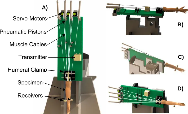
Figure 2.1: Elbow Motion Simulator ... 56

Figure 2.2: Repeatability of Valgus Angulation ... 62

Figure 2.3: Valgus Angle Pathways ... 63

Figure 3.1: Cascade PID Controller with Feedforward Control ... 74

Figure 3.2: Cascade PID Joint Angle Controller ... 76

Figure 3.3: Joint Angle Setpoint vs. Time ... 81

Figure 3.4: Elbow Motion Simulator ... 83

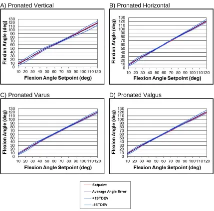
Figure 3.5: Joint angle Performance for Pronated Flexion ... 86

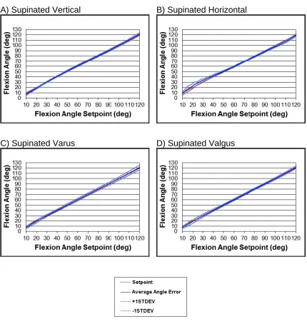
Figure 3.6: Joint angle Performance for Supinated Flexion ... 87

Figure 3.7: Joint angle Performance for Pronated Extension ... 88

Figure 3.8: Joint angle Performance for Supinated Extension... 89

Figure 3.9: Absolute Joint angle Error for Pronated Flexion ... 90

Figure 3.12: Absolute Joint angle Error for Supinated Extension ... 93

Figure 4.1: Joint Coordinate Systems ... 108

Figure 4.2: Elbow Flexion and Forearm Rotation SDAs ... 110

Figure 4.3: Kinematic Pathways ... 114

Figure 4.4: Inter-Subject Variability ... 115

Figure 5.1: Simulated Olecranon Fracture Levels ... 126

Figure 5.2: Anterior and Posterior Triceps Repairs ... 127

Figure 5.3: Triceps Extension Strength Test ... 129

Figure 5.4: Elbow Joint Laxity vs. Olecranon Resection ... 131

Figure 5.5: Extension Strength vs. Triceps Muscle Tension ... 131

Figure B.1: Servo-Motor Actuator and Instrumented Motor Mount ... 158

Figure B.2: Load vs. Time Performance Curve ... 161

Figure C.1: Kinematic pathways in the Vertical Position ... 166

Figure C.2: Kinematic pathways in the Horizontal Position ... 166

Figure C.3: Kinematic pathways in the Varus Position ... 167

Figure C.4: Kinematic pathways in the Valgus Position ... 167

Figure C.5: Inter-Subject Variability of Valgus Angulation... 168

Figure C.6: Inter-Subject Variability of Internal Rotation ... 169

A

BBREVIATIONS

,

S

YMBOLS AND

N

OMENCLATURE

AC/DC ... alternating electrical current / direct electrical current aSDA ... average screw displacement axis cx ... “x” component of position vector cy ... “y” component of position vector cz ... “z” component of position vector

DOF ... degrees-of-freedom dp ... differential change in muscle/tendon position p dθ ... differential change in joint angle θ HULC ... Hand and Upper Limb Centre Hz ... Herts (unit of frequency) IE ... magnitude of internal-external joint rotation MOSE ... Multiple Orientation Simulator for the Elbow P ... position vector p ... muscle/tendon position PID ... proportional integral derivative PPC ... proportional pressure controller psi ... pounds per square inch (unit of pressure) R ... rotation matrix r01 ... component of rotation matrix from 0th row and 1st column

SD ... standard deviation SDA ... screw displacement axis T ... transformation matrix

... transformation of body wrt ref (reference) t ... time

ttrans ... transition time

VV ... magnitude of varus-valgus angulation or joint laxity wrt ... with respect to, meaning relative to a reference frame X ... magnitude of translation along the “x” coordinate direction ref

Z ... magnitude of translation along the “z” coordinate direction θ ... angle of rotation

ΔPosition ... change in position

ΔTension ... change in tension ^ ... over a vector label denotes a unit vector º ... degrees (unit of rotation) ± ... plus or minus; prefixes magnitude of one standard deviation

Δ ... (delta) indicating change

1

C

HAPTER

1

–

I

NTRODUCTION

OVERVIEW: This chapter begins with a synopsis of elbow joint

anatomy and biomechanics, followed by an overview and comparative

discussion of two common joint motion simulation techniques: in-vitro

vs. in-silico. Previously developed in-vitro simulators presented in the

literature are described. Issues concerning the preparation and integrity

of cadaveric tissues are then discussed, followed by an examination of

spatial coordinate systems and the measurement and analysis of elbow

joint motion. This chapter concludes with the rationale for performing

this work, and the objectives and hypotheses.

1.1

E

A

Anatomy of the elbow which is pertinent to this discussion includes all structures which govern and affect elbow motion. There are three classes of such anatomy: osteology (bony structures), ligaments, and musculature.

1.1.1

O

The elbow’s osseous anatomy consists of three bones: the humerus, radius, and ulna. Three articulations are formed between those bones: the ulnohumeral, radiohumeral, and proximal radioulnar articulations (Figure 1.1). These articulations allow for simultaneous elbow flexion-extension and forearm rotation (pronation-supination) motions. The axis of rotation for flexion-extension passes through the centers

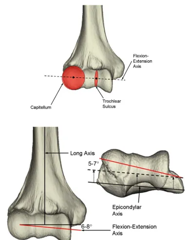
of the capitellum and trochlea (Figure 1.2) (Morrey, 2000). It is angled an average of 6-8° valgus with respect to the medial-lateral axis of the humerus.

1.1.1.1 Humerus

Figure 1.1: Osteotology of the Elbow

A

B

Figure 1.2: Flexion-Extension Axis of the Elbow Joint

(A) The flexion-extension axis (FEA) passes through the center of the capitellum and the center of the trochlear sulcus. (B) The FEA is both 6-8° valgus and 5-7° internally rotated with respect to the humerus. Right arm shown.

forming one joint, this complex geometry allows for two distinct joint rotations (Flexion-extension and pronation-supination). The medial, spool-shaped surface, is the trochlea,

which articulates with the greater sigmoid notch of the ulna, and is covered by 300° of articular cartilage (Morrey, 2000; Shiba et al., 1988). This surface provides the articular

bearing for flexion-extension motion. The trochlear sulcus is a smaller diameter waist in the middle of the trochlea, and forms a track which keeps the greater sigmoid notch of the ulna centered. Laterally, the capitellum is a nearly spherical structure, which articulates with the concave dish of the radial head. It is covered by approximately 180° of articular cartilage, and provides the bearing for both elbow flexion-extension and forearm rotation (pronation-supination). Two extra-articular bony outcroppings, called the medial and lateral epicondyles, serve as attachment sites for the medial and lateral collateral ligaments, and for the muscles of the forearm and hand (Morrey, 2000).

1.1.1.2 Radius

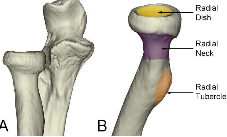
At its most proximal aspect, the radial head has a nearly spherical concave articular surface called the radial dish. The radial dish is entirely covered with cartilage and articulates with the capitellum to allow for forearm rotation (pronation-supination). The cylindrical perimeter of the radial head is covered with 240° of articular cartilage that articulates with the lesser sigmoid notch of the proximal ulna to form the proximal radioulnar joint (PRUJ). The anterolateral portion does not articulate with the ulna and is devoid of articular cartilage, which coincides with the approximate 180° range of forearm rotation. The radial tubercle is a bony outcropping distal to the radial head, which serves as the insertion of the biceps tendon (Figure 1.4) (Morrey, 2000).

1.1.1.3 Ulna

The proximal ulna has two articular surfaces: the greater and lesser sigmoid notches. The guiding ridge of the greater sigmoid notch fits into the track of the trochlear sulcus of the distal humerus. It is angled 30° posteriorly, and is terminated by the olecranon process posteriorly, and by the coronoid process anteriorly. The lesser sigmoid notch is the ulnar half of the proximal radioulnar joint (PRUJ), and has 60-80° of

Figure 1.3: Osteology of the Distal Humerus

Figure 1.4: Osteology of the Proximal Radius

The coronoid and olecranon processes engage their corresponding fossae on the distal humerus at full flexion and extension respectively (Figure 1.5).

1.1.2

L

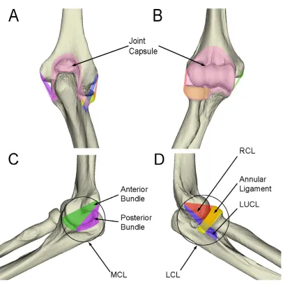
Two major ligamentous structures, the medial and lateral collateral ligaments, contribute to primary stabilization of the elbow. The medial collateral ligament has three components: the anterior, posterior, and transverse bundles. The anterior and posterior bundles originate from the medial epicondyle of the humerus. Their ulnar attachments are much broader. The anterior bundle attaches to the sublime tubercle on the coronoid process. The posterior bundle, though less defined, attaches more posteriorly along the medial aspect of the proximal ulna. The transverse bundle attaches to the ulna only, and currently has no known function (Figure 1.6) (Morrey, 2000).

The lateral collateral ligament has four components. The lateral ulnar collateral ligament (LUCL) originates from the lateral epicondyle of the humerus, coincident with the flexion-extension axis, and attaches to the crista supinatorum tubercle of the ulna. It also blends with the annular ligament, which wraps around the radial head and neck and attaches to the anterior and posterior rims of the lesser sigmoid notch. The radial collateral ligament (RCL) originates from the lateral epicondyle and also blends with the annular ligament. A variable accessory collateral ligament is sometimes described, which originates from the crista supinatorum and blends with the annular ligament (Figure 1.6) (Morrey, 2000).

The collateral ligaments each consist of collagen bundles which provide stability in various directions. Each bundle has fibres which are orientated according to the primary tensile direction for which the bundle offers stability. The bundles themselves are heterogeneous structures composed of a combination of collagen and elastin. Ligaments are viscoelastic (Ohman et al., 2009) which makes their mechanical behaviour

Figure 1.5: Osteology of the Proximal Ulna

(A) Lateral view of the proximal ulna. (B) The proximal ulna consists of the olecranon process, greater and lesser sigmoid notches, and the coronoid. The olecranon process (red) is the insertion of the triceps tendon. The greater sigmoid notch (green) articulates with the humeral trochlea. The coronoid process (purple) forms the anterior prominence of the guiding ridge of the greater sigmoid notch. The lesser sigmoid notch (yellow) articulates with the radial head to form the proximal radioulnar joint. Right arm shown.

Lesser Sigmoid Notch

Figure 1.6: Ligaments and Capsule of the Elbow

1.1.3

E

J

C

The three articulations of the elbow are encapsulated by a single soft tissue structure called the elbow joint capsule. The capsule attaches superiorly of the distal humeral articulations, and encapsulates the radial head, neck, and coronoid process anteriorly. Posteriorly, the capsule attaches around the perimeter of the olecranon process of the ulna, and encloses the olecranon fossa on the humerus (Morrey, 2000). The capsular tissue integrates with the elbow joint’s ligamentous structures, giving the impression of a thickening of the capsule medially and laterally (Figure 1.6). The capsule is a broadly encompassing, non-directional structure with regions being taut or slack depending on the position of the elbow, offering stability in the presence of varying directions of joint load. The anterior capsule is taut in extension and the posterior capsule in flexion (King et al., 1993b).

1.1.4

M

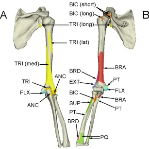
Several muscles originate from the distal humerus and cross the elbow joint before inserting on the forearm and hand (Currier, 1972; Morrey, 2000). These muscles produce elbow flexion-extension, forearm pronation-supination, and flexion-extension of the wrist and fingers (Figure 1.7).

1.1.4.1 Flexors

Figure 1.7: Muscles Crossing the Elbow Joint

the elbow flexion moment when the forearm is supinated. The brachioradialis originates from the lateral supracondylar ridge of the humerus between the triceps and brachialis, and inserts distally at the radial styloid (Morrey, 2000). Though it has the longest moment arm of the flexors, it also has the smallest cross section, thus making the brachioradialis the weakest of the three flexor muscles (An et al., 1981; Murray et al., 1995; Pigeon et

al., 1996).

1.1.4.2 Extensors

The elbow extension moment is generated principally by a single muscle, the triceps. As its name implies, it has three heads. The long head originates from the scapula at the infraglenoid tubercle. The lateral head originates on the lateral intermuscular septum and humerus. The medial head originates broadly from the posteromedial humeral shaft and medial intermuscular septum. All three heads merge to form a single large tendon that inserts at the olecranon process of the ulna (Morrey, 2000).

1.1.4.3 Pronators

Two muscles generate a pronation moment of the forearm (pronator teres and pronator quadratus). The pronator teres has two origins, one at the medial epicondyle is the common flexor-pronator origin. The other is at the coronoid process of the ulna. The muscle passes beneath the brachioradialis to its insertion between the middle and proximal thirds of the radius. It is a strong pronator, and also contributes slightly to the flexion moment. The pronator quadratus is a short, flat muscle that originates at the distal ulna and inserts at the distal radius, running transversely to the forearm on the volar aspect. It is a weak pronator but also provides stability through compression of the distal radioulnar joint (Gordon et al., 2004; Morrey, 2000).

1.1.4.4 Supinators

insertion on the posterior aspect of the proximal radius (Morrey, 2000). The supinator is not as strong as the biceps brachii, but its location is mechanically advantageous for generating a supination moment. Also due to its isolated function, the supinator can be active throughout the flexion range.

1.2

E

K

&

B

1.2.1

K

The flexion-extension axis of the elbow is located anterior to the humeral shaft. As mentioned previously, is defined as an axis through the centers of the capitellum and the trochlear sulcus (Amis et al., 1979b). A full range of flexion for most subjects is

approximately from 0° (full extension) to 145° (Figure 1.8A) (Morrey, 2000). Many subjects can obtain some hyperextension, which is indicated by a negative flexion angle. The actual flexion range attainable for a subject can be affected by the bulk of soft tissue present, prior disease or trauma, and the ligamentous laxity of the individual. Generally, four principal positions of flexion-extension are simulated (Figure 1.9).

With respect to forearm rotation, the ulna remains stationary while the radius pronates and supinates around it. However the motion of the radius is not purely circumferential about the ulna. Rather, the distal radius encircles the distal ulna, while the proximal radius pivots about its own center. Thus the radius crosses the ulna volarly in full pronation. A normal subject can obtain 150-160° of forearm rotation (Figure 1.8B) (Morrey, 2000).

In addition to the principal motions of the elbow articulations (i.e. flexion and

Figure 1.8: Elbow Motions

Figure 1.9: Positions of Upper Extremity Motion Testing

Studying elbow flexion-extension with the gravity load vector in the (A) vertical, (B) horizontal, (C) varus, and (D) valgus positions, provides us with kinematic data in four principal functional positions. Left arm shown.

B) Horizontal

D) Valgus C) Varus

1.2.2

S

Elbow stability is dependent on ligamentous, osseous (the interlocking shape of the articulations) and dynamic (muscular) stabilizers (Morrey and An, 1983; King et al.,

1993c). The articular surfaces of the elbow are highly congruent. This osseous geometry contributes to the relatively high degree of stability enjoyed by the elbow, compared to some other major joints such as the knee and shoulder. Both static and dynamic stabilizers contribute to the overall stability of the elbow.

1.2.2.1 Static Stabilizers

A major source of stability is the congruency between the articular surfaces of the three joints that make up the elbow. The greater sigmoid notch conforms closely to the curvature and complex contours of the trochlea, which when reduced, provides a smooth hinge with resistance to medial-lateral and anterior-posterior translations.

The coronoid and olecranon processes at the terminals of the greater sigmoid notch, are osseous features which provide stability under certain conditions. The coronoid process anteriorly acts as a buttress when it engages the coronoid fossa at full flexion. This prevents posterior subluxation of the ulna on the humerus. It also serves as an important ligamentous attachment (see below). The olecranon process posteriorly contributes to varus and valgus angular stability when it engages the olecranon fossa at full extension.

1.2.2.2 Dynamic Stabilizers

All the muscles that cross the elbow joint provide dynamic stability. Muscle activation compresses and reduces the three elbow joints, causing their articular surfaces to conform and their proper function to be realized. The common extensor origin and the flexor-pronator origin also have a role in stabilizing the elbow that is not fully clarified. However, instability does correlate with the extent of injury to one or both of these muscular origins (Morrey, 2000).

1.3

E

J

K

Kinematics is the branch of classical mechanics that describes the motion of bodies (objects) without consideration of the forces that cause the motion. Numerous studies have used joint motion kinematics as a means to quantify the biomechanical characteristics of the elbow in both in-vivo and in-vitro models. The importance of the

collateral ligaments as elbow joint stabilizers have been evaluated in terms of varus-valgus elbow laxity (Morrey and An, 1983; Olsen et al., 1996a; Sojbjerg et al., 1987b;

Dunning et al., 2001b; King et al., 1993b). Others have measured the contribution of

partial and total elbow joint implants to varus-valgus and internal-external rotation pathways of the ulna relative to the humerus(An, 2005; Itoi et al., 1994; King et al.,

1994; King et al., 1999; O'Driscoll et al., 1992a; Pomianowski et al., 2001a; Stokdijk et

al., 2003). Kinematic measurements have been used to design and evaluate implant

designs and also surgical interventions and repairs. Conditions which cause non-physiological joint motion pathways can lead to osteoarthritis or undue ligament and muscle strain. Malalignment of the osseous articulations can also cause regions of bone to become shielded from normal compressive forces, which can lead to bone weakening and bone loss due to resorption. In the case of joint implants; malalignment of implant components to native joint rotation axes or articular surfaces can also be revealed by changes in joint motion (Itoi et al., 1994; King et al., 1993a; O'Driscoll et al., 1992a;

Schuind et al., 1995; An, 2005; Morrey and An, 1983; Olsen et al., 1996a; Sojbjerg et al.,

1.3.1

M

T

M

A variety of technologies and techniques have been employed to measure and record in-vitro joint motion. Mechanical linkages attached to bone segments can measure

joint rotations. These can be employed as rotary variable transducers, or rotary (shaft) encoders. It is difficult to accurately align these devices to the joint rotation axes, and any misalignment results in an underestimation of the actual joint rotation. It is possible to measure translations with linkages as well. However, 6DOF (6 degrees of freedom) measurements would require six linkages with six transducers for each bone of interest.

Biplane Fluoroscopy and Roentgen Stereophotogrammetric Analysis (RSA) has been used to record 6DOF joint motion (Li et al., 2008; Hanson et al., 2006). While

traditional RSA techniques require impaction of small spherical metal beads into the surface of bones, new model-based registration techniques do not (Bey et al., 2006; de

Bruin et al., 2008). The common use of biplane fluoroscopy in clinical diagnostics and

surgical navigation, also makes it well suited for some in-vitro investigations. However,

the bulk and cost of the equipment and the use of radiation make it difficult to justify its generalized use for in-vitro joint motion studies.

Dynamic 6DOF spatial tracking devices are available in a few forms that are easily categorized by the physics they employ. These are sonic, optical and electromagnetic. Sonic trackers (usually ultrasonic) can suffer from signal blocking and interference. Accuracies are generally in the range of 2-3 mm RMS, and sonic reflection from walls and objects can be problematic (Welch, 2002).

“see”. They are often wired for power and synchronization, but can be wireless with battery power, though this means a much larger active target. Passive targets have retro-reflective surfaces which reflect light (usually infrared) that is emitted from the cameras. Their retro-reflective property ensures that the light emitted from each camera is reflected back to the camera so that the location of the target can be “seen”. Since every passive target in the field of view is illuminated, objects are generally identified by having different geometric configurations of passive targets. This can lead to large collections of passive targets compared to active targets which can be identified by illumination sequence. The location of both active and passive targets are measured according to their centroid, and thus they represent single points, which is why an object needs at least three of them to be located in space. Pattern targets generally are high-contrast (usually black and white) patterns or 2D bar codes which are imaged in the viewable spectrum. Targets are distinguished by their unique patterns. Pattern recognition algorithms identify the targets and track their position and orientation. The pattern origin can be defined arbitrarily.

Electromagnetic trackers employ a field transmitter which generates an electromagnetic field in the working volume (Figure 1.10). Generally, the transmitter has three independent field coils, one for each global coordinate axis Tr(X, Y, Z). Receivers,

much smaller than the transmitter, also contain three independent coils, one for each axis of the receiver’s local coordinate system. The receiver’s coils act as antennas in the transmitted field. These trackers do not suffer from target occlusion and the receivers are generally quite small, making this modality easy to implement. However, sources of electromagnetic noise and induced eddy currents in metallic objects can interfere with their measurements (Welch, 2002).

At the time of this writing, there are two dominant spatial tracking modalities: electromagnetic and optical. In the fields of in-vivo gate kinematics, optical tracking with

Figure 1.10: Electromagnetic Tracking System

The transmitter (Tr) emits an electromagnetic field from each of its three coordinate coils. Each field induces currents in the antennae of any receivers (Rc) within range. The electronics unit (EU) measures the induced currents and interprets their relative magnitudes as positions and rotations of the receiver relative to the transmitter. trakSTAR™ (Ascension Technologies Inc., Burlington, VT) shown.

Field Receiver (Rc1) X

Y Z

X Y

Z

Field Transmitter (Tr)

Field Receiver (Rc2) X

Y Z Electronics Unit

(EU)

PC Workstation

For in-vitro study applications such as those described in this work, both

electromagnetic and optical trackers enjoy a similar amount of acceptance. All the data presented herein was collected using either a Flock of Birds® or trakSTAR® from Ascension Technologies Corp. (Burlington, VT) electromagnetic tracker. More recently, the Optotrak Certus® (Northern Digital Inc., Waterloo, ON) has been used for motion data collection and computer-navigated orthopaedic surgical protocols. The Certus is the most accurate 6DOF tracker available, and its position measurements are more reliable than electromagnetic trackers when there are accompanying rotations. However, due to the various positions in which this simulator can perform elbow flexion, occlusion of optical targets is a major limitation of the Certus system. Thus, electromagnetic tracking remains a practical choice for in-vitro studies of this nature.

1.3.2

O

B

A vector space is created from an orthonormal basis. That is a set of mutually perpendicular vectors of magnitude one. These are the vectors that define the Cartesian coordinate directions in which kinematic descriptors will be quantified. Vector spaces will henceforth be referred to as coordinate systems. These can be thought of as being global or local (body-specific). Body-specific coordinate systems allow the 6DOF location and orientation of a body to be quantified in space (the global system) or relative to other bodies (Figure 1.11). Any orthonormal coordinate system is easily created by first defining two vectors, then by calculating the vector cross product between them which gives a third vector that is perpendicular to both of the initial vectors.

Figure 1.11: Orthonormal Basis

Three mutually perpendicular unit vectors form an orthonormal basis or coordinate system. The location (blue dot) is defined in terms of components along the three axes (x, y, z).

Y

X

The simplest body is a particle, represented by a point and assumed to have negligible dimensions. A particle requires three quantities to specify its location in 3D space relative to a reference coordinate system. Thus, the location of a particle can be described by translations in three principal coordinate directions (x, y, z), and is said to have 3DOF degrees of freedom. Because a particle has negligible dimensions, pure rotation of the particle is not described, since the result of a rotated point leads to the same point. The next level of complexity in kinematics describes the motion of bodies with non-negligible dimensions. Such a body can be thought of as a collection of particles that are fixed relative to each other - whose relative positions are time invariant.

These collections of particles are referred to as rigid bodies. A rigid body can undergo translations and rotations (Figure 1.12). As with a particle, the location of a rigid body can be quantified by translations in the three Cartesian coordinate directions (i.e. x,

y, z). Since a rigid body has non-zero dimensions, its location is defined to a point fixed relative to the rigid body, which corresponds to the center of its local coordinate system. Then the orientation of the rigid body can be quantified by three rotations about the coordinate axes of the reference coordinate system. Thus, an unconstrained rigid body is said to have 6DOF.

1.3.3

B

S

C

S

Figure 1.12: Rigid Body Pose

Three linear translations along coordinate axes (x, y, z) and three rotations about those axes. These six degrees of freedom (DOF) completely define the pose (location and orientation) of the rigid body (object). Shown is the trivial case where the rigid body coordinate system is coincident with the global coordinate system. The general case will be described later.

Z

X Y

Figure 1.13: Bone Fixed Local Coordinate Systems

The humerus is rigidly mounted relative to the transmitter and the humeral coordinate system is created relative to the transmitter. The ulnar coordinate system is created relative to its corresponding field receiver. By convention, the +X and +Z axes point proximally and medially, respectively, for both bones. To maintain a right hand rotation convention, the +Y axis points anteriorly for a right arm and posteriorly for a left. The origins of the coordinate systems correspond to the joint rotation center. Left arm shown.

Y X

Z Humerus (H)

Ulna (U) X

Y Z

Field Transmitter (Tr)

Field Receiver (Rc) X

Y

1.3.3.1 Anatomy-Derived Coordinate Systems

A common method for creating the direction and position vectors is by using a digitizing stylus probe. A field receiver is mounted to a stylus probe, whose tip position vector is known relative to the receiver. The stylus is used to probe the surface of the bones, while the receiver pose transforms are recorded. The surface of the bone relative to the bone’s reference receiver is calculated using the known stylus tip position vector. This method is called “digitizing”. Surface digitization can also be performed using non-contact methods such as laser scanners. Bony features that are digitized include the articular surfaces and landmarks that can describe the long axes. The usual intent is to digitize bony features that describe the flexion axis and long axis, so that the resulting fixed coordinate systems are aligned with the functional axes of the bones (Wu et al.,

2005). These are referred to as Anatomy-Derived CS (Coordinate Systems).

Although Anatomy-Derived CS have enjoyed widespread use in biomechanics research; they also have significant limitations. Anatomy-Derived CS are based on the precept that joint function follows from joint form (Brownhill et al., 2006). However, in

the case of the elbow; the anatomy-derived flexion axis has been found to deviate systematically from the axis about which the ulna rotates (Brownhill et al., 2006). This is

likely due to the fact that elbow motion is not only a function of its articulations, but also includes contributions from muscle activity, as well as guiding support from the capsule and ligaments.

1.3.3.2 Motion-Derived Coordinate Systems

Another method for creating bone fixed coordinate systems is by using joint motion recordings. By analyzing the joint motions, the flexion and forearm rotation axes can be calculated. These are often referred to as helical or Screw Displacement Axes (SDAs), and they have been shown to accurately represent the rotation axes of flexion and forearm rotation. By using these rotation axes and their intersection, bone fixed coordinate systems can be created as per (Ferreira et al., 2010) and described in Chapter

1.3.4

C

T

Before meaningful and clinically relevant joint kinematic data can be interpreted, they must first be calculated from the pose (position and orientation) records collected by the spatial tracking system. Each pose record represents a time frame of positions and orientations of each spatial tracker target with respect to the tracker’s origin. The tracker’s origin can be the center of an electromagnetic field transmitter, a camera or system of cameras, or any object or abstract locale, depending on the spatial tracking modality. Thus, coordinate transformations are needed to convert this data into joint kinematic data.

1.3.4.1 The Transformation Matrix

Coordinate systems will be represented numerically with transformation matrices. A transformation matrix T, is a 4 by 4 (16 element) array of real numbers (Figure 1.14). It is composed of three parts: a 3 by 3 (9 element) rotation matrix R, a translation vector c, and the last row [0, 0, 0, 1]. The rotation matrix, is itself composed of three parts: the three orthonormal direction vectors (x, y, z). The unit direction vectors of the body’s local coordinate system are inserted vertically into the rotation matrix portion of the array. This syntax ensures that the matrix represents the transformation of the body relative to its reference coordinate system (Figure 1.12). It is worth noting that the horizontal rows of the rotation matrix represent the orientation of the reference system relative to the body, which is equal to the result of the inverse operation. Therefore, the transpose of the rotation matrix is equal to its inverse. This is a convenient property because the transpose operation is much less computationally expensive than matrix inversion.

Figure 1.14: The Transformation Matrix

The transformation matrix is denoted by an upper case T. The preceding subscript and superscript represent the rigid body and its reference coordinate systems respectively. The rotation matrix (blue) portion is composed of the three orthonormal vectors of a rigid body’s local coordinate system described in the space of a reference coordinate system, and represents the rigid body’s orientation relative to that reference coordinate system. The position vector (red) represents the location of the rigid body relative to the reference coordinate system. The last row on the bottom (green) facilitates matrix operations.

r00 r01 r02 cx

r10 r11 r12 cy

r20 r21 r22 cz

0 0 0 1

^

X Y^ Z^

In this work, we are dealing with rigid bones. Thus, we will use only translation and rotation operations, which result in rigid body transformations. Thus, a rigid body will always have the same size, shape and aspect ratio before and after the transformation is applied. The orthonormality of the direction vectors in the rotation matrix portion is the property that limits transformations to rigid body rotation only. This is the reason for using the orthonormal basis for all coordinate systems.

1.3.4.2 Transformation Chain

A typical setup for data collection is one where a receiver is mounted on the ulna and the humerus is rigidly mounted relative to the transmitter (Figure 1.13). During motion recording, raw pose data for the receiver is recorded relative to the field transmitter. The pose data is represented in the form of transformation matrices. Where

represents the pose of the ulnar receiver relative to the field transmitter. and represent the pose of the humerus and ulna relative to the transmitter and receiver, respectively. The following sequence shows the matrix multiplications needed to

generate , which represents the transform of the ulna into the humerus’ coordinate system.

(Eq. 1.1)

Notice that the preceding subscript and superscript of adjacent transforms are equal, meaning that those transforms involve a common body or coordinate system. By writing the equation in this way, the common intermediate body “cancels out”, leaving a transform of the remaining bodies. Using this logic, it is possible to automate this process.

The transformation chain can easily be expanded to include more moving bodies, or deeper reference bodies. The above transform represents the ulna relative to the humerus, but one can easy add other anatomical structures such as the radius and hand, simply by appending a T matrix for each bone segment to the end of the chain. The same can be done at the beginning of the chain if one wants to include the scapula, the trunk, and other related structures.

H

UT

=

Rc

U T

Tr

Rc T

H

Tr T

H

UT

Rc

U T

Tr

H T

Tr

1.3.5

E

A

The Euler angle method is commonly used to quantify joint kinematics. Euler angles describe the attitude of a body with an ordered sequence of rotations about the body’s local coordinate axes (Craig, 1989; Karduna et al., 2000; Small et al., 1992;

Woltring, 1991). The change in attitude of a body (i.e. ulna) from an initial orientation

that is coincident with a reference frame (i.e. humerus) to any subsequent position is fully

described by defining three angles termed (yaw, pitch, roll). These angles describe rotations about the bone-fixed axes of the Z, Y and X axes of the ulna respectively. The rotation angles are applied in sequence and the order of that sequence is important.

Since the rotation angles are referenced with respect to the body’s own axes, as the body is rotated, the axes of subsequent rotations get moved by rotations earlier in the sequence. The rotation sequence representing ulnar motion is Z→Y→X in the ulna’s own reference frame. Since the ulnar reference frame is moving, this means that after the rotation sequence is applied, the first rotation will have occurred about the humeral Z axis, and the last rotation about the final location of the ulnar X axis. In the final orientation, the second rotation appears to have occurred about an arbitrary axis which is generally no longer coincident with any of the humeral or ulnar axes. The axis of the second rotation was called the “line of nodes” by Euler (Goldstein H., 1950) because it contains the two orbital nodes which represent the intersections of conceptual orbital arc paths within the first and third rotation planes. Grood and Suntay termed it the “floating axis” (Grood and Suntay, 1983) because it is not fixed to the rigid body as are the X, Y, Z axes, which makes its location (observed globally) dependent on the magnitude of the first rotation angle.

numerical precision of computers, rotations near 90º will also exhibit symptoms due to gimbal lock. We avoid this problem by choosing a rotation sequence that cannot lead to a second rotation of 90º. In the elbow, this is accomplished by defining a direction perpendicular to the elbow flexion axis as the second Euler rotation axis. Functionally, the ulna can achieve a flexion angle of 90º, but rotation about the anterior-posterior axis of the ulna is limited by ligamentous stabilizers. Only a catastrophically disrupted and dislocated elbow could achieve a rotation near 90º about this axis.

1.3.6

J

M

P

Kinematic descriptors are necessary to quantify joint motions in ways that are clinically relevant. To facilitate this, it is useful to align the local bone segment coordinate system with relevant anatomical or functional axes, such as the bone’s long axis or flexion axis. This alignment is crucial if the Euler angle descriptions are to be accurate. The bone local coordinate system provides the axes for Euler rotations. Thus, misalignment between the coordinate system and the functional axes of the joint will cause a component of one joint rotation to be falsely interpreted as contributing to another rotation of interest, and concurrently, a component of the joint rotation of interest will be lost (Piazza and Cavanagh, 2000). This is because the coordinate misalignment will cause a rotation about a true functional axis to be represented by more than one coordinate rotation, thus being divided into smaller components.

1.3.6.1 Varus-Valgus Angulation and Joint Laxity

An elbow joint motion of clinical interest is the varus or valgus angle of the ulna relative to the humerus (Figure 1.15A). If the ulnar and humeral coordinate systems are coincident, then varus-valgus (VV) angulation is the adducted-abducted (toward-away from body) angular deviation of the ulnar long axis from the humeral sagittal plane about the anterior-posterior axis of the ulna. Since this is not about a rotation axis of the elbow, it is useful as a measure of elbow function in the evaluation of the integrity of osseous and soft tissue stabilizers. Thus VV angulation serves as a very common kinematic descriptor of elbow performance as a function of flexion angle.

Elbow joint laxity is another important descriptor of joint function. Varus-valgus laxity is quantified as the difference in the varus and valgus angles between the varus and valgus gravity loaded positions (Figure 1.9). It is essentially a measure of how loose the joint is, or how effective the joint stabilizers are.

1.3.6.2 Internal-External Rotation

Internal or external rotation of the ulna relative to the humerus is another useful kinematic descriptor of elbow function. Internal-External (IE) rotation is defined as ulnar rotation about its own long axis (Figure 1.15B) – not to be confused with forearm rotation (radius about the ulna). IE rotation is not an articular degree of freedom, though some degree of ulnohumeral IE rotation does occur normally. Thus, the degree of IE rotation can also be used to evaluate the condition of osseous and soft tissue stabilizers.

1.3.6.3 Joint Translations

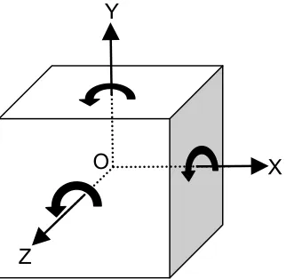
Figure 1.15: Elbow Kinematics

These are the kinematic descriptors of elbow motion. (A) Varus-valgus (VV) angulation. (B) Internal-external (IE) rotations. (C) Proximal-Distal, Medial (out of page), Lateral (into page), and Anterior-Posterior translations. Right arm shown.

Posterior Proximal

1.4

S

E

J

M

Elbow joint motion that occurs naturally in vivo can be studied through

simulation. Although no method of joint simulation has yet been developed which is a perfect elbow joint analog, there is still a strong scientific rationale for employing simulations. Simulation allows investigators to isolate and control various aspects of a specimen and its environment, and in so doing to create a more understandable or analyzable system. For example surgical procedures and implants can be tested and optimized using simulators, prior to their application in patients. Furthermore, many studies cannot be performed in vivo due to issues of safety and practicality.

Testing devices and simulators (if defined as systems which aim to model joint motion and loading) have been developed to mimic joint motion and loading for various activities. None of the presently available devices can fully model in-vivo loading.

However, they do provide a useful basis to compare various rehabilitation protocols and surgical procedures.

As regards the elbow, there are four principal positions of the upper extremity in which flexion-extension is generally simulated. These are the vertical (gravity dependent), horizontal, varus and valgus positions (Figure 1.9). Testing in all four of these positions covers a broad range of externally applied moments that are experienced by the elbow during normal use.

In-vitro joint simulators have been developed to mimic kinematics and loading in

the laboratory for various motions. While modeling the in-vivo state is difficult to

1.4.1

I

-S

I

-V

E

J

S

Simulation of elbow motion can be performed virtually (in-silico) using computer

models, or physically with cadaveric specimens (in-vitro) by using specialized devices to

move the specimen and record the characteristics of its motion (i.e. kinematics). Each

method of simulation has its advantages and challenges.

The clear advantage of in-silico simulation is that virtual anatomical models can

be an inexpensive and readily reusable source of specimens, while avoiding the challenges and expense of maintaining a biohazard test facility. Virtual models, allow investigators to control and adjust every variable that the model is designed to account for, which makes them valuable for a variety of studies. However, as with all virtual simulators, in-silico models of elbow joint motion must incorporate many assumptions

and simplifications of anatomical functions and properties in order to successfully execute the simulations (Klein et al., 2007). These simplifications are not due to a lack of

computing power. Rather they are necessary in order to compensate for the complexities of the elbow as a system of interacting muscles, bones, and other soft tissues with complex and still incompletely understood mechanical properties. For instance, consider the capsuloligamentous and tendinous structures previously described in Sections 1.1.2 Ligaments and 1.1.3 Elbow Joint Capsule. These tissues have complex geometries with constituent components that offer stability in multiple and varying directions. Their mechanical performance is rate dependent due to viscoelastic properties, and their degree of stabilization is direction dependent due to heterogeneous material composition (Quapp and Weiss, 1998). These are compound structures – having a number of sub-bundles – with complex and variable geometries.

In-silico models must incorporate numerous assumptions in order to compensate

for an incomplete knowledge of the tissues involved. For example, ligament properties are often considered identical to that of tendons for the purpose of modeling mechanical properties (Benjamin et al., 2002; Cooper and Misol, 1970; Evans et al., 1990). This is

Furthermore, the properties of tendons are not completely understood. In measuring patellar tendon properties in vivo, (Couppe et al., 2009) noted that studies based on

cross-sectional designs, such as theirs and many others, have inherent limitations which leave them at risk of type II errors (Couppe et al., 2009). The main reason given was the wide

variation in tendon mechanical properties among the population (Magnusson et al.,

2001). Effects related to aging are also inconclusive due to disagreement in the literature; with some experiments suggesting that tendon compliance increases, others that it decreases, and yet others that it remains unchanged with age (Carroll et al., 2008; Couppe

et al., 2009; Karamanidis and Arampatzis, 2006; Kubo et al., 2003; Kubo et al., 2007a;

Kubo et al., 2007b; Mademli et al., 2008; Mian et al., 2007; Morse et al., 2005;

Onambele et al., 2006).

These deficits in the current knowledge base necessitate compromises when modeling each discrete structure (i.e. ligament, tendon, muscle, etc.). However, elbow

function involves complex interaction among many such structures, and this interaction of incompletely defined mechanical properties may compound modelling errors.

The advantage of in-vitro simulation is that the unknowns discussed above

concerning tissue properties and mechanical behaviours, and the complex interactions among the various tissues can be left to function as they normally would in vivo. Also,

using specimens selected from the actual human population automatically incorporates the wide variations in osseous anatomy, ligament and tendon properties (Ohman et al.,

2009) that occur among individuals.

Furthermore, certain studies must be performed on real tissue. For example, the results from evaluating surgical repairs are more realistic when those repairs are performed in vitro, because there are normal variations in outcomes that are caused by

the practical aspects of surgery. Variables such as surgeon performance, variations in tissue properties and others are nearly impossible to model. If the performance of a surgical repair is being evaluated, then the hands-on nature of that repair must be present in the study protocol if a proper evaluation is to be achieved. If the evaluation includes measurements of motion or internal forces, then in-vitro simulation is the only option.

evaluated using in-vitro experiments (Baldwin et al., 2009; Halloran et al., 2005; Laz et

al., 2006; Mommersteeg et al., 1996; Sathasivam and Walker, 1997; Patil et al., 2003;

Saikko and Calonius, 2002). Thus, the future of in-silico models is dependent on the

continued development of in-vitro simulators. Until the day comes when virtual models

achieve near perfect simulations of elbow joint function, there will be a need for in-vitro

simulation, since it is logical that the perfect in-silico model may one day be validated by

the perfect in-vitro simulator.

1.4.2

P

M

S

Elbow joint function can be simulated with passive motion, in which an investigator manually moves the forearm through a range of motion, while dependent variables such as kinematics or joint forces are measured. For in-vitro tests, this method

can be used with or without simulated muscle forces. This technique has implications to post-trauma and post-surgical rehabilitation protocols, in which therapists employ passive motions to help patients regain elbow function.

One of the first passive simulators included a handle mounted to the ulna by which an investigator manually moved the forearm (Sojbjerg et al., 1987a; Sojbjerg et

al., 1987b). The handle was instrumented with strain gauges in order to measure the

applied moments, allowing the investigator to apply a varus-valgus or internal-external moment to the forearm while passively flexing or extending the elbow. Sojbjerg et al.

investigated the contribution of the radial head and annular ligament (Sojbjerg et al.,

1987b) and the medial collateral ligament to the stability of the elbow (Sojbjerg et al.,

1987a). This device formed the basis for several more investigations into elbow stability following radial head excision and ligament disruption (Olsen et al., 1994; Olsen et al.,

1998; Olsen et al., 1996b; Jensen et al., 1999).

Stokdijk et al. (2003) fixed the humerus to a rigid frame, and employed manual

passive elbow flexion. An electromagnetic tracking system recorded ulnohumeral motion, and SDAs were used to evaluate total elbow replacement in a cadaveric model (Stokdijk et al., 2003).

static weights applied to the tendons of the brachialis, biceps and triceps muscles. These forces were 5% of the maximum potential force for those muscles and less than the physiologic forces needed to move the joint. They were only intended to stabilize the joint, as this can improve joint congruity and likely produce more physiologically accurate kinematics in-vitro. Elbow flexion was still generated manually by an

investigator. The humeral mount allowed axial rotation of the humerus, which was used to model varus and valgus gravity loaded flexion (Figure 1.9) (Morrey et al., 1991).

Subsequently, several elbow studies utilized this simulator (O'Driscoll et al., 1992a;

O'Driscoll et al., 1992b; Itoi et al., 1994; King et al., 1993a; Pomianowski et al., 2001a;

Pomianowski et al., 2001b).

Another passive motion simulator used a DC electric motor and pulley aligned with the flexion axis, which applied an external force directly to the bones of the forearm in order to generate elbow flexion. Static weights were applied to the biceps, brachialis and triceps muscles, in order to simulate muscle loads, as with the above passive simulator. This system was used in conjunction with an electromagnetic tracking system to quantify ulnohumeral passive motion kinematics with SDAs (Screw Displacement Axes) (Bottlang et al., 2000a; Bottlang et al., 2000b). While the motion generated by this

device is not performed manually, it is also not representative of in-vivo active motion,

since the moments causing rotation about the flexion axis are not generated by tension loads crossing the elbow joint, in a manner consistent with physiological muscle activation. Rather, this form of simulation can be described as automated passive motion. The advantages of this over manual passive simulation are improved repeatability and constant angular joint rotation (Bottlang et al., 2000b).

Another automated passive simulator used stepper motors to apply external loads directly to the humerus and forearm. Four stepper motors applied three orthogonal joint translations, and forearm rotation. Flexion angle was preset and the apparatus allowed free varus-valgus angulation. This device was used to evaluate elbow joint stability under various conditions (Deutch et al., 2003b; Deutch et al., 2003a; Deutch et al., 2003c;

Jensen et al., 2003).

joint torques, or known displacements in order to quantify joint stability. These represent a type of stop-and-go method of modeling elbow joint kinematics (Seiber et al., 2009;

Fern et al., 2009; Hull et al., 2005). With these, static muscle loads can also be simulated

(Fern et al., 2009; Hull et al., 2005). However, there are limitations in interpreting these

measurements as being joint kinematics, since “kinematics” would suggest that the joint is actually moving. Passively moving the joint to various flexion angles and fixing it in place while taking kinematic measurements may not account for all the subtle and changing tissue interactions.

Passive motion with simulated muscle loads, whether manual or automated, produces a muscle loading model that is a balanced static system of loads. However,

in-vivo active motion is clearly a system not in equilibrium, but rather a dynamic

unbalanced system of loads, which generates the flexion-extension moment about the elbow flexion axis. Thus, in-vitro passive motion is not a complete and physiologically

accurate model by which to simulate in-vivo motion.

1.4.3

A

M

S

In order for an in-vitro simulator to be categorized as active, it must produce

flexion-extension in a sense that is representative of in-vivo motion. Thus, the

flexion-extension moment generated about the elbow flexion axis must be developed from forces crossing the elbow joint. This can only be achieved by loading the muscles described in section 1.1.4. Simulating muscle activation to generate elbow flexion-extension has benefits. Balanced loading of the triceps, biceps and brachialis has been demonstrated to significantly stabilize the intact elbow in in-vitro studies (King et al., 1994). Simulated

variable muscle loading has also been shown to have an important stabilizing effect on the intact elbow (Johnson et al., 2000). This stabilizing effect is even more evident

following transection of primary stabilizers such as the MCL or LCL (Armstrong et al.,

2000; Dunning et al., 2001b).

It is incumbent on the designers to employ muscle forces that are consistent with muscle effort during in-vivo motion. However, this is not a trivial problem. Unknown