On the numerical scheme employed in gyrotron interaction simulations

On the numerical scheme employed in gyrotron interaction

simulations

K. A. Avramides1, A. K. Ram2, O. Dumbrajs3, S. Alberti4, T. M. Tran4, and S. Kern5

1

National Technical University of Athens (part of HELLAS), School of Electrical and Computer Engineering, Association EURATOM-Hellenic Republic, GR-15773, Zografou, Greece

2

Massachusetts Institute of Technology, Plasma Science and Fusion Center, Cambridge, Massachusetts 02139, USA

3

University of Latvia, Institute of Solid-State Physics, Association EURATOM-University of Latvia, Kengaraga Street 8, LV-1063, Riga, Latvia

4

Ecole Polytechnique Fédérale de Lausanne (EPFL), Centre de Recherches en Physique des Plasmas (CRPP), Association EURATOM–Confédération Suisse, CH-1015, Lausanne, Switzerland

5

Karlsruhe Institute of Technology (KIT), Institute for Pulsed Power and Microwave Technology (IHM), Association EURATOM-KIT, Kaiserstrasse 12, 76131 Karlsruhe, Germany

Abstract. We report on the influence of the numerical scheme employed in gyrotron interaction simulations. Results obtained with the Crank-Nicolson scheme are compared with those obtained with the Backward Time – Centred Space (BTCS) fully implicit scheme. We present realistic cases where, for discretisation parameters in the range usually used in gyrotron simulations, the results can be very different. Hence, the numerical scheme used can be responsible for obscuring the underlying physics if its convergence is not tested carefully.

1 Introduction

Gyrotrons are the leading microwave sources for high-frequency waves needed for plasma heating and current drive in magnetic confinement fusion experiments. The European Gyrotron Consortium (EGYC) is developing a 170 GHz gyrotron in support of Europe’s contribution to ITER [1-3]. In a gyrotron, a helical electron beam guided by a magnetostatic field delivers energy to a high-frequency (RF) wave through electron cyclotron resonance. Simulations of the beam-wave interaction are important for guiding gyrotron design and in support of the experiments. In order for the interaction codes to be used as designing and/or supportive tools, fast simulations are necessary.

There are four European interaction codes, available at EGYC, based on the slow-time scale approximation and thus capable of fast simulations: EURIDICE [4], SELFT [5], COAXIAL [6], and TWANG [7]. The results of the codes are in agreement in the majority of cases that have been tested. Some discrepancies that appear are understood and attributed to the difference in the interaction models. However, in some cases of interest, the results of COAXIAL have been significantly different from those of the other codes. This triggered an extensive investigation which indicated that this discrepancy was a consequence of the difference in the employed numerical scheme: COAXIAL uses a scheme which is first-order in time, whereas the rest of the codes use schemes that are second-order in time. To clarify the situation, EURIDICE was modified in second-order to provide the option to use

This is an Open Access article distributed under the terms of the Creative Commons Attribution License 2.0, which permits unrestricted use, distribution, and reproduction in any medium, provided the original work is properly cited.

DOI: 10.1051/ C

either of the two schemes. The results confirmed that the previously observed discrepancies were due to the difference in the numerical scheme. In the next sections we present the beam-wave interaction equations and the numerical schemes for their integration, together with realistic cases where, for discretisation parameters in the range usually used for efficient simulations, the two schemes give results that are different not only quantitatively, but also qualitatively.

2 Interaction model and numerical schemes

Many variants of the slow-time-scale, self-consistent model for the beam-wave interaction in the gyrotron cavity exist in the literature ([8] and references therein). The model consists of the equations for the electron motion and the equations for the field profiles of the TE modes of the cavity, which are interacting with the electrons. For the purpose of the present discussion, we use the model in the code COAXIAL [9]:

(

)

2

1 B sexp s s

s dp

i p p i f i

dζ ζ ψ

   

+ _ − − ∆ _ =

∑

(

)

2 2 2

2 2

0 0 exp 4

s s s

s s s s

f f I

i f p i d d

π π

δ ζ ψ θ ϕ

ζ τ π

∂ ∂ _{ }

− + = _− ∆ + _

∂ ∂

∫ ∫

The physical process described by (1)-(2) is the interaction, at the fundamental cyclotron frequency, of a weakly relativistic electron beam having no spreads in electron energy, velocity and guiding centre, with a set of TE modes that are close to cut-off and in resonance with the beam. It is assumed that the cavity walls are perfectly conducting and that the axial electron momentum is constant. The latter approximation is valid for weak tapering of the magnetostatic field.

Detailed definition of the normalised quantities in (1)-(2) can be found in [9]: p(ζ) is the electron complex transverse momentum normalised to its initial absolute value, fs(ζ, τ) is a complex function describing the envelope of the RF field axial profile of the s-th mode, ζ (∝z) and τ (∝t) denote axial distance along the cavity, and time, respectively. The quantities p and fs are average quantities over the cyclotron period (gyro-averaged, slow-time-scale equations). The parameter ∆_{B(ζ) describes the} magnetic field tapering along the cavity axis and the parameter δs(ζ) accounts for the mild axial inhomogeneity of the cavity wall. The normalised current Is(ζ, τ) incorporates the coefficient describing the coupling between the s-th mode and the electron beam, along with the stored energy coefficient. The parameter ∆_{s is the frequency mismatch of the s-th mode and ψs (τ,φ) is the mode} phase, where φ is the azimuthal position of the electron guiding centre. The initial condition for (1) is

p(0) = exp(iθ), 0 ≤ θ <2π_{, and the boundary conditions for (2) are reflectionless boundary conditions} at the carrier frequency of the s-th mode, i. e. at the frequency of the fast oscillations of the mode.

The models used in EURIDICE, SELFT and TWANG are more complicated than (1)-(2), accounting in a more elaborate way for several physical effects by dropping some of the assumptions of (1)-(2). However, regarding the scope of this paper, these differences do not play an important role. As a result, what we state by using (1)-(2) as a reference model applies also to the other models. The equation of motion (1) is solved in the codes using some Runge-Kutta or equivalent scheme. Here we will concentrate on the numerical solution of the equation (2) for the field profile, which is a two-dimensional partial differential equation of the form:

2

2 ( , ) ( , )

( ) ( , ) ( , )

A z t A z t

i z A z t S z t

t z δ

∂ ₌∂ _{+ +}

∂ ∂

space-discretisation step, respectively. Using the notation ( , ) n

k n k

A z t ≡A , we can come up with the following two finite difference schemes [10] for the numerical integration of (3):

Backward Time – Centred Space scheme (BTCS):

1 1 1 1

1 1

1 1

2 2

n n n n n

n n

k k k k k

k k k

A A A A A

i A S

t z δ

+ + + +

+ +

+ −

− − +

= + +

∆ ∆

Crank-Nicolson scheme (C-N):

1 1 1 1

1 1

1 1 1 1

2 2

2 2

1 1

2 2

n n n n n n n n

n n n n

k k k k k k k k

k k k k k k

A A A A A A A A

i A S A S

t z δ z δ

+ + + +

+ +

+ − + −

−  − +   − + 

= _ + + _+ _ + + _

∆ _ ∆ _{ } ∆ _

The BTCS scheme, also known as the fully implicit scheme, is second-order in space and first-order in time, whereas the C-N scheme is second-order in both space and time. The code COAXIAL uses the BTCS for the integration of the field equation, whereas EURIDICE and SELFT use the C-N. TWANG uses a finite element method, which is also second order in time and space, like the C-N.

3 Numerical results

3.1 Dynamic after-cavity interaction

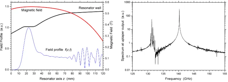
Recently, in some cases where the simulated interaction region is not confined to the gyrotron cavity but it also incorporates the non-linear uptaper after the cavity, dynamic after-cavity interaction (ACI) has been observed [11]. In dynamic ACI, a mode is interacting with the beam in the cavity at some frequency and, at the same time, the mode is also interacting with the beam at the non-linear uptaper at a different frequency. The existence of two frequencies results in a strong beating which is apparent both in the field profile and in the output power. An example of dynamic ACI in the 1 MW, 140 GHz gyrotron for W7-X [12], as simulated by EURIDICE, is shown in Figure 1. Along with the operating frequency at 140 GHz, parasitic frequencies at ~131 GHz are excited due to interaction at the uptaper, deforming the RF field profile at this area (z > 80 mm).

Dynamic ACI is predicted, with good agreement, by EURIDICE, SELFT and TWANG in several cases. However, COAXIAL did not predict such interaction. An extensive investigation excluded the differences in the employed interaction models from being the reason for the discrepancy, and indicated the difference in the numerical schemes used. This became apparent from a convergence

Fig. 1. Simulated dynamic after-cavity interaction in the W7-X gyrotron.

Left: Resonator wall, magnetic field, and absolute field profile of the operating TE28,8 mode versus

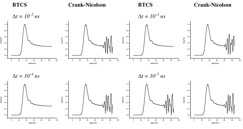
study performed with EURIDICE, after its modification to be able to use both C-N and BTCS. Results are presented in Figure 2. The test case is the design of a 1 MW, 170 GHz gyrotron, operating at the TE32,9 mode, which is the EU fall-back solution for ITER [1]. The results reveal that,

compared to the C-N, the BTCS needs a three orders of magnitude smaller time-discretisation step ∆_{t to show the dynamic ACI. This results in prohibitively long computation time. Following this} result, COAXIAL was finally able to simulate dynamic ACI by using an adequately small ∆_t.

In order to illustrate more the dissipative action of the BTCS which suppresses dynamic ACI, we performed a similar convergence study by enforcing a field profile with ACI as an initial condition

BTCS Crank-Nicolson BTCS Crank-Nicolson

∆_{t = 10}–2 _ns ∆_{t = 10}–3 _ns

0 20 40 60 80 100 120 0.0 0.2 0.4 0.6 0.8 1.0 A b s P ro f zeta(mm)

0 20 40 60 80 100 120 0.0 0.2 0.4 0.6 0.8 1.0 A b s P ro f zeta(mm)

0 20 40 60 80 100 120 0.0 0.2 0.4 0.6 0.8 1.0 A b s P ro f zeta(mm)

0 20 40 60 80 100 120 0.0 0.2 0.4 0.6 0.8 1.0 A b s P ro f zeta(mm)

∆_{t = 10}–4 _ns ∆_{t = 10}–5 _ns

0 20 40 60 80 100 120 0.0 0.2 0.4 0.6 0.8 1.0 A b s P ro f zeta(mm)

0 20 40 60 80 100 120 0.0 0.2 0.4 0.6 0.8 1.0 A b s P ro f zeta(mm)

0 20 40 60 80 100 120 0.0 0.2 0.4 0.6 0.8 1.0 A b s P ro f zeta(mm)

0 20 40 60 80 100 120 0.0 0.2 0.4 0.6 0.8 1.0 A b s P ro f zeta(mm)

Fig. 2. Study of convergence, vs. the time discretisation step ∆_{t, for BTCS and C-N schemes.}

Test case: 1 MW, 170 GHz gyrotron (EU fall-back solution for ITER), ∆_{z = 0.1 mm,} ∆_{t parameter.}

In the graphs, the absolute field profile of the operating TE32,9 mode vs. the resonator axis is shown.

BTCS Crank-Nicolson BTCS Crank-Nicolson

∆_{t = 10}–2 _ns ∆_{t = 10}–3 _ns

100 101 102 103 104 105 106 107 108 109 110 0 500 1000 1500 2000 2500 3000 P o w e r (k W )

Time (ns)

100 101102 103104 105 106107 108109 110 0 500 1000 1500 2000 2500 3000 P o w e r (k W )

Time (ns)

100 101 102 103 104 105 106 107 108 109 110 0 500 1000 1500 2000 2500 3000 P o w e r (k W )

Time (ns)

100 101 102 103 104 105 106 107 108 109 110 0 500 1000 1500 2000 2500 3000 P o w e r (k W )

Time (ns)

∆_{t = 10}–4 _ns ∆_{t = 10}–5 _ns

100 101 102 103 104 105 106 107 108 109 110 0 500 1000 1500 2000 2500 3000 P o w e r (k W )

Time (ns)

100 101102 103104 105 106107 108109 110 0 500 1000 1500 2000 2500 3000 P o w e r (k W )

Time (ns)

100 101 102 103 104 105 106 107 108 109 110 0 500 1000 1500 2000 2500 3000 P o w e r (k W )

Time (ns)

100 101 102 103 104 105 106 107 108 109 110 0 500 1000 1500 2000 2500 3000 P o w e r (k W )

Time (ns)

Fig. 3. Study of convergence, vs. the time discretisation step ∆_{t, for BTCS and C-N schemes.}

for the field profile f(z, t) and let it evolve over time. The results (in terms of output power) shown in Figure 3, confirm that BTCS needs a much smaller time-discretisation step ∆_{t to converge to the} results of C-N. The power fluctuations have a period of ~0.1 ns, which is the beating period between the operating (170 GHz) and ACI (~160 GHz) frequencies.

At this point we should stress that dynamic ACI is an effect that is currently under extensive analysis regarding both the experimental findings and the capability of the present interaction models and codes to describe it correctly [11-12]. Discussion on the validity of the models and codes in treating dynamic ACI is beyond the scope of this paper, which focuses on the influence of the numerical scheme on the calculations.

3.2 Frequency-tunable gyrotron

In contrast to the dynamic ACI case, the case addressed in this section lies well into the region of validity of the interaction models and codes. It refers to a frequency-tunable gyrotron for Nuclear Magnetic Resonance spectroscopy, enhanced by Dynamic Nuclear Polarisation (DNP-NMR) [13]. The gyrotron operates at the TE7,2 mode at the frequency of about 263 GHz and frequency tuning

can be realised by changing the magnetic field. The frequency tunability is achieved by the successive excitation of higher axial harmonics of the operating mode. The output power remains at a level above 10 W.

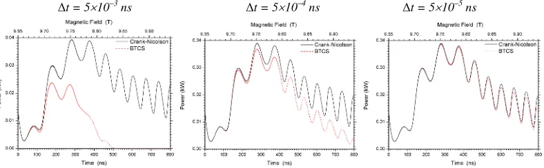
In Figure 4 we show the output power of this gyrotron as a function of time, where the magnetic field is increasing linearly with time from 9.65 T up to 9.94 T. The operating frequency changes correspondingly from 262.93 GHz up to 269.82 GHz. The power fluctuations correspond to the successive excitation of higher axial harmonics of the TE7,2 mode. In this example ohmic losses are

not taken into account. The results are obtained by EURIDICE using both the BTCS scheme and the C-N. Again the BTCS results converge to the C-N results for adequately small time-discretisation step ∆_{t. For larger time-discretisation step BTCS predicts much narrower frequency tunability. The} essential conclusion is that the results of C-N converge to a solution for relatively large time-discretisation step ∆_{t, while the BTCS results obviously depend on the chosen} ∆_{t and converge to the} result of C-N only for very small ∆_t.

4 Discussion

We have compared results of simulations of the beam-wave interaction in gyrotrons for two realistic cases. We use two different numerical schemes - the BTCS fully implicit scheme and the Crank-Nicolson scheme. It is shown that the BTCS needs about three orders of magnitude smaller time-discretisation step ∆_{t in order to converge to the results obtained by the C-N. This makes the BTCS}

∆_{t = 5}×₁₀–3 _ns ∆_{t = 5}×₁₀–4 _ns ∆_{t = 5}×₁₀–5 _ns

Fig. 4. Study of convergence, vs. the time discretisation step ∆_{t, for BTCS and C-N schemes.}

Test case: 10 W, 263 GHz frequency-tunable gyrotron for DNP-NMR, ∆_{z = 0.05 mm,} ∆_{t parameter.}

In the graphs, the output power of the operating TE7,2 mode vs. time is shown.

very inefficient in the simulated cases, as the required simulation time becomes very long. We should expect such behaviour, since the BTCS is first-order in time whereas the C-N is second-order in time. However, in the vast majority of practical cases, such behaviour is not encountered; both schemes give the same results using a time-discretisation step of the order of ∆_{t ~ 10}–1 _{to 10}–2 _ns. Such time-steps are usually used in interaction simulations of mm-wave gyrotrons. This agreement has led to a confidence in both schemes, which, following the results of the present study, needs to be reassessed as far as the BTCS scheme is concerned. The issue requires some special attention because the convergence of the BTCS with the time-discretisation step ∆_{t may be misleading. For} example, in Figure 1, BTCS gives identical results for time-discretisation down to ∆_{t = 10}–4 _ns, which is already two orders of magnitude below the “usual” time-discretisation. Without trying even smaller ∆_{t, one would believe that the BTCS scheme has already converged.}

In [14] it was suggested that, for gyrotron time-dependent simulations, the BTCS may be preferable to the C-N on the grounds that C-N could be numerically unstable over long simulated time intervals. A discussion on this topic is beyond the scope of this paper. However, in the cases we have studied there are no traces of numerical instability for the C-N, i. e., no “exploding” solutions. Furthermore, from our experience using the C-N for a large variety of simulations, we have never faced instability issues.

Acknowledgement

This work was supported in part by Fusion for Energy under Grant F4E-2009-GRT-049 (PMS-H.CD)-01 and within the European Gyrotron Consortium (EGYC), and by the US Department of Energy. The views and opinions expressed herein do not necessarily reflect those of the European Commission. The European Gyrotron Consortium (EGYC) is a collaboration among CRPP, Switzerland; KIT, Germany; HELLAS, Greece; IFP-CNR, Italy.

References

1. F. Albajar et al., EC-15, 10-13 March 2008, Yosemite National Park, CA, USA, Conference Proceedings 415 (2009)

2. J.-P. Hogge et al., Fusion Sci. and Tech. 55, 204-212 (2009)

3. S. Kern et al., EC-17, 7-11 May 2012, Deurne, The Netherlands (this conference)

4. K. A. Avramides, I. Gr. Pagonakis, C. T. Iatrou, and J. L. Vomvoridis, EC-17, 7-11 May 2012, Deurne, The Netherlands (this conference)

5. S. Kern, Numerische Simulation der Gyrotron-Wechselwirkung in koaxialen Resonatoren, PhD Thesis, FZKA 5837, Karlsruhe Institute of Technology (1996)

6. O. Dumbrajs, COAXIAL, Helsinki University of Technology, unpublished (2001)

7. S. Alberti, T M. Tran, K. A. Avramides, F. Li and J.-P. Hogge, 36th Int. Conf. Infrared

Millimeter THz Waves, 2-7 October 2011, Houston ,TX, USA, Conference proceedings Tu5.15

(2011)

8. C. J. Edgcombe, Ed., Gyrotron Oscillators, London: Taylor and Francis, ch. 3-4 (1993) 9. O. Dumbrajs, Y. Kominis, and G. S. Nusinovich, Phys. Plasmas 16, 013102 (2009)

10. J. W. Thomas, Numerical partial differential equations – Finite difference methods, Springer (1995)

11. S. Kern et al., 35th Int. Conf. Infrared Millimeter THz Waves, 5-10 September 2010, Rome, Italy, Conference proceedings We-P.14 (2010)

12. A. Schlaich et al., 36th Int. Conf. Infrared Millimeter THz Waves, 2-7 October 2011, Houston,

Texas, USA, Conference proceedings Th2A.4 (2011)

13. S. Alberti et al., 34th Int. Conf. Infrared Millimeter THz Waves, 21-25 September 2009, Busan,

Korea, Conference proceedings M5E56.0111 (2009)