WR2716
Multiobjective Optimization of Seasonal Operating Rules for Water Grids Using Streamflow
Forecast Information
Stephanie C. Ashbolt1 and B. J. C. Perera2
1Postgraduate Student, Institute of Sustainability and Innovation, College of Engineering and Science,
Victoria University, Footscray, Australia; Postgraduate Student, Commonwealth Scientific and Industrial Research Organisation, Clayton, Australia (corresponding author). E-mail: [email protected]
2Dean, Institute of Sustainability and Innovation, College of Engineering and Science, Victoria University,
Footscray, Australia. E-mail: [email protected]
Abstract
Multi-objective simulation-optimisation is a useful tool for determining operating rules for water supply that are optimal for multiple management objectives and for expected conditions over the planning period. Previous studies have shown the benefits of streamflow forecasts in improving optimised objective performance of reservoir operating rules. This study demonstrates a simple method for incorporating publicly-available streamflow forecast information in operational planning for a water grid. Multi-objective optimisation is used to find operating rules for a case study that are optimal for three management objectives – maximising minimum system storage, minimising operational cost, and minimising spills from reservoirs – and for the forecast inflow scenarios. These forecast-optimised rules are compared to those optimised using inflow scenarios from the historical distribution, representing operation in the absence of forecast
information. The results across four seasonal (3 month) planning periods indicate that, on average, operating rules optimised using forecast streamflow information perform slightly better in terms of the management objectives than those optimised using historical inflow information. Using multiple scenarios of inflow that span the forecast distribution increases the robustness of the operating rules and reduces the risk of under-performance due to forecast inaccuracy. The results suggest that incorporating streamflow forecast
information into multi-objective simulation-optimisation has the potential to provide improvements in seasonal operating rules for a water grid.
Keywords
Introduction
Water supply managers typically need to develop seasonal (3-month) or annual (1 year) short-term operating plans, to identify operating rules that can achieve their desired outcomes. These desired outcomes are typically expressed in terms of multiple management objectives or criteria which aim to maximise water security, minimise energy use, minimise operational cost, or meet environmental flows. Multi-objective simulation-optimisation is a useful tool to determine operating rules that are optimal for multiple management objectives (Ashbolt et al. 2016a; Ashbolt et al. 2014; Kim 2008; Kumphon 2013). The operating rules found using multi-objective simulation-optimisation will be optimal not only for the management objectives, but also for the inflow timeseries that are input to the simulation-optimisation model. Therefore, operating rules may only remain optimal during the planning period if the inflow assumptions in the simulation-optimisation process hold true in reality (Beh et al. 2015; Walker et al. 2013). For this reason, uncertainty in expected inflow should be incorporated into simulation-optimisation to identify options that perform optimally over – are robust to – a range of expected inflow probabilities (Maier et al. 2014).
Multiple inflow scenarios, sampled from the historic inflow record, can be used in simulation-optimisation of the water supply system to identify operating rules that are robust to various inflow possibilities. However, using such historical inflow scenarios assumes no knowledge of the probability of these scenarios in the near future; many may be extremely unlikely based on current catchment conditions (Faber and Stedinger 2001). Streamflow forecasts that reflect both current catchment conditions and the climate outlook over the planning period may suggest different probabilities of inflow. The historic-sampling approach could be updated by selecting inflow scenarios that reflect the forecast probability distribution for the planning period. Used with optimisation, this forecast-based sampling approach should allow operating rules to be tailored for expected conditions over coming months. Although streamflow forecasts are uncertain, they can provide a more honest and risk-aware indicator of future conditions than relying on historical averages (Krzysztofowicz 2001; Piechota et al. 2001); optimising operating rules to multiple scenarios from across the forecast inflow
distribution should improve the robustness of operating rules and system performance if observed inflow volumes deviate from the forecast median (Georgakakos and Graham 2008).
multiple reservoir systems has been shown to improve objective performance. Alemu (2011) found that incorporating streamflow forecasts in multi-objective optimisation improved system performance of 12-month operating rules for a two-reservoir hydroelectric project. Gelati et al. (2013) optimised dual-reservoir releases using a multi-stage single-objective optimisation process to minimise hydropower deficit and meet target storage levels, using a set of 100 stochastic 9 month forecast inflows based on synthetic El Niño-Southern Oscillation (ENSO) data. They found that forecast-optimised operation provided improvements over historical-optimised operation and over rule-curve based operation. Sankarasubramanian et al. (2009a) demonstrated that simulation of water allocation using streamflow forecasts, downscaled from monthly precipitation forecasts, helped to reduce reservoir spill, increase hydropower generation and meet end-of-season target storage when compared to the use of historical values. Gong et al. (2010) demonstrated a simple method to update reservoir rule curves for three reservoirs using simulations based on streamflow forecast probabilities, resulting in a reduction in drought emergency days. Finally, Li et al. (2014) found that using ensemble streamflow forecasts in a stochastic linear programming model helped to reduce deviations from end-of-season target storage for a multi-reservoir system with inter-basin transfers.
These studies have all shown the potential of streamflow forecasts to improve seasonal to annual operating rules for systems of one to three reservoirs. A gap exists in demonstrating the use of forecast information to improve short-term operating rules for larger, more complex, water supply systems. These studies also developed forecast inflows specifically for each case study. An additional opportunity arises to discover whether existing publicly available forecasts, such as those provided by the Bureau of Meteorology in Australia (Australian Government Bureau of Meteorology 2017), can be used in a forecast-based sampling approach to update historically-sampled reservoir inflow data for simulation and optimisation of operating rules.
In Ashbolt et al. (2016a), the authors of this study showed how multi-objective simulation-optimisation can be used to identify optimal annual operating rules for a case study based on the water grid in South East Queensland, Australia. The study showed that multi-objective simulation-optimisation can improve objective performance over the short term compared to a base case of operation using fixed longer-term rules. This formed proof-of-concept of the core part of a framework for short-term operational planning for water grids presented in Ashbolt et al. (2014). However, the operating rules in that study were optimised for a single scenario of historical observed flow, assuming perfect knowledge of inflow volume, which cannot be
of future conditions, particularly in context of publicly-available data such as that provided by the Bureau of Meteorology in Australia. Thus an opportunity exists to demonstrate how this streamflow forecast information can be used to improve multi-objective performance of short-term operating rules for this case study.
Incorporating probabilistic streamflow forecast information into practice remains a key challenge for water supply management (Brown et al. 2015; Pagano et al. 2002; Sankarasubramanian et al. 2009b). However, translating such forecasts to existing simulation-optimisation models and data can increase the likelihood of adoption of forecasts by industry (Gong et al. 2010, Whateley et al. 2015). Therefore this study aims to demonstrate how a simple method can leverage publicly-available, probabilistic streamflow forecast information to update an existing multi-objective simulation-optimisation model and improve objective performance. The number of scenarios is limited to reduce the computational burden and thus run-time. This simple method involves sampling the historical inflow data currently available for the simulation-optimisation model, based on a distribution of forecast inflow volumes such as those provided by the Australian
Government Bureau of Meteorology (2017). This method follows two of the three uncertainty modelling paradigms outlined by Maier et al. (2016): use of best available knowledge (publicly available streamflow forecasts); and quantification of uncertainty (probabilistic distribution of forecasts). It also aligns with the future research directions discussed by (Maier et al. 2014), by providing an example of how optimisation with uncertainty could be used in real decision-making, within a reasonable timeframe. The method is applied to the multi-objective simulation-optimisation model and water grid case study developed in Ashbolt et al. (2016a) to optimise operating rules for a short-term seasonal planning timeframe corresponding to the forecast data availability. These operating rules are expected to improve objective performance for the planning period, compared to operating rules optimised to historical inflow. This improvement is expected since operating rules are optimised for forecast inflow volumes that should average closer to the observed flow than the average or median historic inflow volume. The use of multiple scenarios from the forecast distribution is expected to improve robustness of operating rules if observed inflow deviates significantly from the forecast median, compared to the alternative of a single historic or forecast inflow scenario.
Case study
connected to 48 demands via multiple supply paths along a network of streams and one- and two-way pipelines that cross catchment boundaries (inter-basin transfers). Operating rules need to be determined for this water grid to guide operation of key supply and transfer systems. These operating rules aim to meet three management objectives: maximising water security, minimising total operational cost, and minimising total spills from reservoirs. The operational planning period used in Ashbolt et al. (2016a) and in recent operational plans for South East Queensland (Seqwater 2014) is one year, with operating rules assessed for objective performance over a longer five-year horizon.
Currently, streamflow forecasts are available for catchments located within the case study area, published online on a monthly basis by the Australian Government Bureau of Meteorology (2017). However, these streamflow forecasts have a seasonal three-month horizon, shorter than the annual planning period originally required for the case study. For the purposes of the current study, a revised three-month seasonal
operational planning period is examined to enable direct use of the streamflow forecast information. In the future, the Bureau of Meteorology plans to extend the seasonal forecasts to a 1 year horizon (Wang et al. 2014); these updated forecasts can then be used in the case study simulation-optimisation model. Regardless of the length of the planning period used, the method presented in this study can be repeated every month to reflect updated forecast inflow information.
Four retrospective (past) seasonal planning periods are examined for the case study: July-September 1989, 1991, 1997, and 2000. These four seasonal planning periods are chosen to assess the potential
improvement in operating rule performance due to incorporation of streamflow forecast information, when compared to using historical inflow information. They were also chosen based on differences in forecast accuracy and volume, to assess the impact of these factors on performance. Here, forecast accuracy is measured as the difference between observed flow and the forecast median, as a single-year variant of the forecast skill score used by the Bureau of Meteorology, described in the following sub-section (Available streamflow forecasts). Two of the planning periods are selected based on their higher forecast accuracy, with the forecast median relatively close to observed inflow. The other two planning periods are selected based on their lower forecast accuracy, with the forecast median significantly different to observed inflow. All four planning periods cover the same July-September season, to avoid any variability in results due to differing historic forecast skill or inter-seasonal variability. The four planning periods are examined from the
forecast information described in the following sub-sections.
Problem formulation and simulation-optimisation model
In Ashbolt et al. (2016a), a multi-objective optimisation problem was formulated for the case study. Apart from the difference in retrospective planning periods and inflow scenarios (described in more detail in the
Method), the problem formulation and simulation-optimisation model for this study are unchanged from that described in Ashbolt et al. (2016a). A brief overview is provided here; the reader is referred to that paper for further detail.
The aim of the case study is to determine operating rules that are optimal in terms of the three management objectives of maximising water security, minimising total operational cost, and minimising total spills from reservoirs. Objective performance is calculated using the three objective functions shown in Equations 1-3. Where multiple inflow scenarios are used, the aim of optimisation is minimise or maximise the sum of the objective functions across simulations using the different inflow scenarios. Since there are trade-offs
between these objectives, e.g. an increase in water security might be obtained at the expense of an increase in operational cost and spill volume, the results of multi-objective optimisation will be multiple possible operating options that represent trade-offs between the three objectives.
The water security objective is measured by an objective function determining the minimum system storage over the planning period. Minimum System Storage is calculated as:
𝑀𝑖𝑛𝑖𝑚𝑢𝑚 𝑆𝑦𝑠𝑡𝑒𝑚 𝑆𝑡𝑜𝑟𝑎𝑔𝑒 = min (𝑆𝑆𝑡 𝑓𝑜𝑟 𝑡 = 1, … , 𝑇) Equation 1
where t is a time-step of the planning period of length T; and SSt is the sum of storage volumes in the
surface water storages (in megalitres) for the time-step t. This objective function is to be maximised.
The total operational cost objective concerns costs occurring due to treatment, pumping, production of manufactured water, and switching direction of the two-way pipelines. It is measured by the objective function, Total Cost, calculated as:
𝑇𝑜𝑡𝑎𝑙 𝐶𝑜𝑠𝑡 = ∑
𝑡=1𝑇[∑
𝑓∈𝐹𝑈𝐶
𝑓,𝑡∗ 𝐹𝑅
𝑓,𝑡+ ∑
𝑝∈𝑃($40,000𝐴𝑈𝐷 ∗ 𝑆
𝑝,𝑡)]
Equation 2
where t is a time-step of the planning period of length T; f is a node or link in the network (e.g., treatment plant, pumping station, or desalination plant) of the entire set F with an associated flow-dependent treatment, pumping or production unit cost UCf,t($AUD/ML) and FRf,t (megalitres/day) on timestep t; and p is a two-way
a pipeline p on timestep t compared to timestep t-1 (0 = no switch or 1 = switch). The total cost is the sum of operational costs over all timesteps of the planning period. This objective function is to be minimised.
The total spill volume objective is measured by an objective function, calculated as:
𝑇𝑜𝑡𝑎𝑙 𝑆𝑝𝑖𝑙𝑙 𝑉𝑜𝑙𝑢𝑚𝑒 = ∑
𝑇𝑡=1[∑
𝑟∈𝑅𝑆𝑉
𝑟,𝑡]
Equation 3where t is the time-step of the planning period of length T; r is the reservoir of the entire set R; and SVr,t is
the spill volume from the reservoir r on timestep t, in ML. The total spill is the sum of spill volumes over all reservoirs and timesteps of the planning period. This objective function is to be minimised.
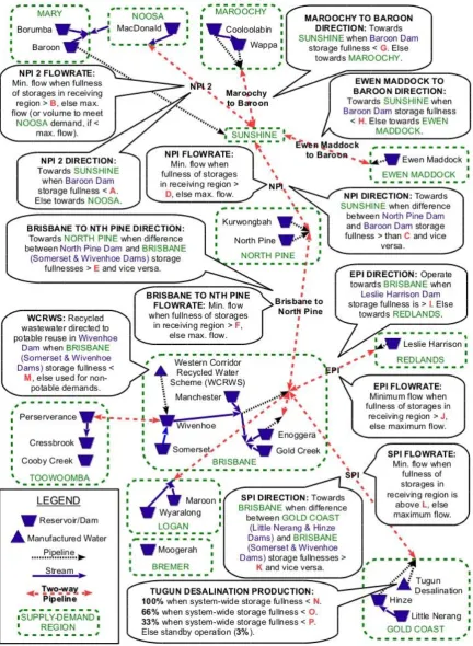
A daily timestep simulation-optimisation model of the case study was constructed using eWater Source (Dutta et al. 2013). This model was chosen based on its ability to simulate and multi-objective optimise operating rules for a complex water grid (Ashbolt et al. 2014). The key features of the supply system represented in the model are illustrated in Figure 1. This figure shows a schematic representation of the major water sources, demand regions, and pipelines; the operating rules to be optimised; and the decision variables which constitute the operating rules. Not shown in this figure, but included in the model are 39 inflows and 48 demand nodes, groundwater supplies, weirs, smaller pipelines and streams, and a number of environmental flow requirements. Daily inflow timeseries are available for 39 inflow sites in the model, disaggregated from monthly calibrated timeseries covering 117 years from 1890-2007. There are sixteen operating rules, outlined in the callout boxes in Figure 1, which govern the direction and flowrate of the seven two-way pipelines, production volume of the desalination plant, and whether or not the potable recycled water is directed for reuse in the reservoir or to non-potable demands. These operating rules contain sixteen decision variables, which form a set [A, B, C, … P] also shown in Figure 1. These decision variables
Figure 1: Schematic of the case study network, showing operating rules (call out boxes) for major
Available streamflow forecasts
The Bureau of Meteorology (BoM) is the Australian national weather, climate and water agency. Each month, it provides three-month-ahead seasonal streamflow forecasts for a number of catchments across the country, including within the case study area (Australian Government Bureau of Meteorology 2017). These forecasts provide a probability distribution of three-month seasonal total predicted inflow volumes, and use a Box-Cox transformed multivariate normal distribution to model intersite correlations (Wang et al. 2009). The
probabilistic forecasts are composed of an ensemble of 5000 equally probable forecast volumes, produced from simulations using a Bayesian Joint Probability (BJP) model (Wang et al. 2009). The BJP model is a probabilistic statistical forecast method that predicts streamflows at multiple sites based on multiple and uncertain predictors such as climate outlook and initial catchment conditions (Robertson and Wang 2009). In addition to the probabilistic forecast distribution, an indication is given of the skill score, i.e. the historical accuracy of the model for that season. The Root Mean Square Error in Probability (RMSEP) indicates the level of skill for each of the forecast sites and catchments, as the square root of the average difference between the historical probabilities of the observed value and forecast median (Wang and Robertson 2011). A RMSEP of <10 is deemed very low skill, 10-20 low skill, 20-40 moderate skill, and >40 high skill. Forecast skill depends on the initial catchment conditions, and the time of year (Wang et al. 2011); where the skill score is very low, the historical probability distribution is used for the forecast.
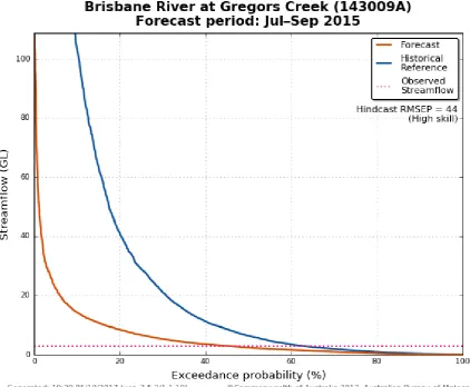
An example of a forecast for one of the sites in the case study area is shown in Figure 2, for the July-September 2015 season at the confluence of Brisbane River and Gregors Creek, upstream from Wivenhoe Dam. This season and site has a high skill, with a RMSEP of 44. Figure 2 shows the probability of
Figure 2: Example forecast and historic flow duration curves for Brisbane River at Gregors Creek, a forecast site within the case study area. Observed flow is indicated by the dashed line. (Reprinted from Australian Government Bureau of Meteorology 2017).
Forecast sites and spatial grouping of inflows
Seasonal three-month streamflow forecasts are available from the Bureau of Meteorology (BoM) within four of the eleven case study catchments. These BoM forecast sites can be used to provide information about the forecast inflow distribution, to sample historical inflow at nearby inflow sites represented in the simulation-optimisation model. Four forecast sites are listed in Table 1, Column 2. To identify which forecasts should be linked to which model inflow sites, the 39 model inflow sites are grouped to the four forecast sites, on a per-catchment basis. The first step in this spatial grouping is to pair the four forecast sites with four model
catchment group representatives (Table 1, Column 3), which are the most highly correlated inflow sites in the
July-September inflow with the four model catchment group representatives, as shown in Table 1, Column 4. Correlation was used rather than physical distance as it is a more reliable measure of similarity in streamflow (Archfield and Vogel 2010). Kendall's tau-b rank correlation coefficient was used to measure this correlation; this measure is non-parametric and can be used for time-series with zero-flow values (Wang and Robertson 2011). The four catchment groups in Table 1 are used to connect forecast and historic inflow distributions to model inflow scenarios as described in the Method.
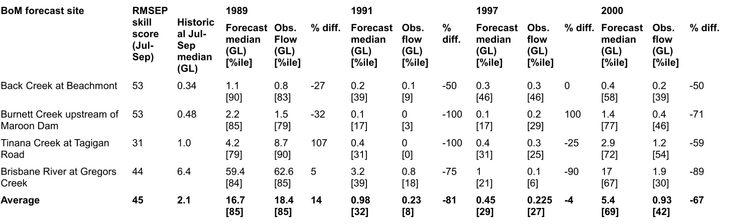
For the July-September forecast season of the four case study retrospective seasonal planning periods, the historical forecast skill score of the four BoM forecast sites is moderate to high (Table 2, Column 2). Three of the four forecast sites have Root Mean Square Error in Probability (RMSEP) indicating high skill (>40), with the Tinana Creek forecast site having moderate skill (20-40). Due to these relatively high skill scores, the forecasts for these sites would typically be expected to be fairly reliable. The forecast volumes and observed flows for the two retrospective planning periods at the BoM forecast sites are shown in Table 2. Each of the planning seasons and sites has different forecast inflow and accuracy relative to the historic median. Both the July-September 1989 and 2000 planning periods have average forecast median flows significantly above the average historic median (85th and 69th percentile). However the July-September 1989 had higher
accuracy, with an average difference of 14% between the observed inflow and forecast median for the four case study forecast sites. On the other hand, the July-September 2000 observed flow had lower accuracy, with the observed inflow 67% lower on average than the forecast median, closer to or below the historic median. Both the July-September 1991 and 1997 periods had forecast median flows below the historic medians. However, the 1997 planning period had higher accuracy in the forecast, with an average difference of -4%. The observed flows for July-September 1991 were even lower than the forecast medians, with an average difference of -81%. In summary, a decision-maker planning for the July-September season would expect reasonably high skill in the forecast on average. However, the forecasts for the case study planning periods had varying levels of accuracy, with both under- and over-prediction of inflows and observed flows both lower and higher than the historic median.
Method
Aim and overview
historic probability distributions may be 'correct', objective performance is optimised over multiple inflow scenarios to explicitly address this uncertainty (Krzysztofowicz 2001). Comparing forecast- and historic-optimised operating rules should show whether or not integrating streamflow forecast information into simulation-optimisation can improve objective performance. These forecast- and historical-optimised operating rules are also compared to operating rules optimised using a single scenario of observed inflow over the planning period. This allows the improvement of forecast-optimised operating rules over historic-optimised to be assessed relative to theoretical maximum performance that could be obtained using a perfect forecast of observed flow. These comparisons are done separately for the four retrospective planning periods described in the previous section. Comparing the relative improvement obtained from forecasts for the four planning periods should show the impact of forecast accuracy on objective performance, and the ability of optimisation using probabilistic inflow scenarios to ameliorate this impact by improving the robustness of operating rules.
The method used in this study contains four steps:
1. Developing forecast, historical and observed inflow timeseries scenarios for input to the simulation-optimisation model, by sampling from historical inflow data.
2. Developing forecast, historical and observed optimisation problem formulations using the respective inflow scenarios from Step 1 and the problem formulation and simulation-optimisation model. 3. Multi-objective optimisation to obtain forecast-, historical- and observed-optimised Pareto sets of
operating rules, one set for each of the optimisation formulations from Step 2.
4. Using compromise programming, a multi-criteria analysis technique (Zeleny 1973), to select and compare one operating option each from the three Pareto sets from Step 3, using preferences on the objectives.
More detail on each of the steps are provided in the following subsections.
Developing inflow scenarios (Step 1)
Step 1 of the method involves developing inflow scenarios for three optimisation formulations: forecast, historical and observed. Each of these problem formulations requires daily inflow timeseries at each of the 39 inflow nodes in the simulation-optimisation model. The forecast and historical optimisation formulations require multiple scenarios of inflow timeseries, generated from the forecast and historical distributions for the relevant planning periods, to capture the uncertainty in expected inflows. Optimising to these inflow
These are the inflows that have 90%, 75%, 50%, 25% and 10% probability of exceedance respectively. Whilst a greater number of inflow scenarios is desirable, this limited number of scenarios restricts the run-time of the multi-objective optimisation model to a manageable run-timeframe. Unlike the forecast and historical optimisation formulations, the observed optimisation formulation requires just a single timeseries of observed data for the four planning periods. The following sections describe the method for developing forecast, historic and observed inflow scenarios. This method is repeated for each of the planning periods.
Forecast inflow scenarios
A simple method is used here to develop inflow scenarios for the forecast optimisation formulation, based on the available data. This available data includes: forecast and historic flow duration curves of three-month total inflows at the four BoM forecast sites; and daily 117-year (1890-2007) modelled historical inflow timeseries at the 39 simulation-optimisation model inflow sites described in the Case study section. The 39 model inflow sites do not correspond directly to the forecast sites, both in their location and timestep. Therefore, the 10th, 25th, 50th, 75th, and 90th percentile forecast streamflow volumes cannot be used directly as model inputs. Instead, the forecast flow volumes at the forecast sites are spatially mapped to daily forecast timeseries for each of the model inflow nodes using the flow duration curves at the forecast and model catchment group representative sites listed in Table 1.
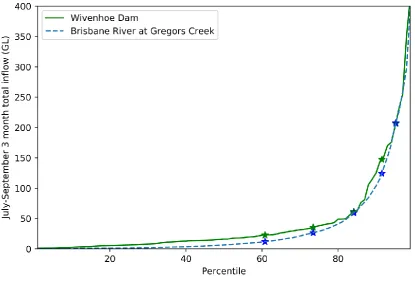
Figure 3: Flow-duration curve representing the historic distribution of total July-September inflow at Brisbane River at Gregors Creek), forecast site for Catchment Group 4 (dashed line). The five stars on this line
indicate the 10th, 25th, 50th, 75th, and 90th percentile forecast inflow volumes for the July-September 1989
planning period (y-axis) and their corresponding percentiles within the historic July-September distribution (x-axis). The solid line indicates the flow-duration curve for the same period at Wivenhoe Dam, the model catchment group representative for Model Catchment Group 4. The stars on this line indicate forecast inflow volumes (y-axis) corresponding to the forecast percentiles for Gregors Creek (x-axis).
Stage three of developing forecast inflow scenarios involves translating the forecasts for each of the BoM forecast sites to inflow volumes for each of the model catchment group representatives, as per the
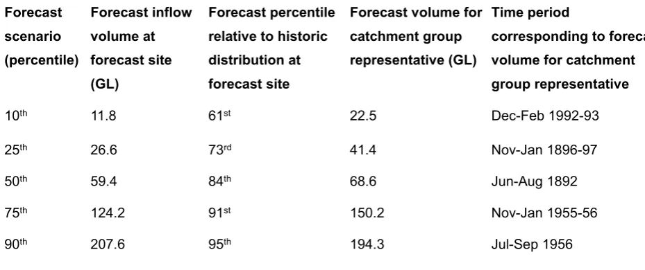
catchment group pairings in Table 1. This translation is achieved by determining the inflow volumes from the historic distribution of the model catchment group representatives that correspond to the historic-adjusted forecast percentiles from the second stage (e.g. the stars on Wivenhoe Dam flow-duration curve in Figure 3). Essentially, for a given forecast inflow scenario, the same (historic-adjusted) percentile flow at the forecast site is used as for the model catchment group representative site. This means that although the magnitude of inflows at the model sites may be different to those at the forecast sites, the percentile or quantile of that flow is the same. This approach is used because the two sites are spatially close and highly correlated, and thus would be expected to have similar relative flow. Thus a 10th percentile forecast volume of 11.8 GL for Brisbane River at Gregors Creek forecast site (Table 3 Columns 1 & 2) is translated to a Wivenhoe Dam Inflow 10th percentile forecast volume of 22.5 GL (Table 3 Column 4): both volumes sit at the same relative point in the historic distribution, ie. the 61st percentile.
Finally, stage four of the method involves translating the three-month forecast scenario volumes for the four model catchment group representatives to daily inflow timeseries at each of the 39 model inflow nodes. This is achieved by determining the periods of the historic 117 year daily inflow timeseries for the four model catchment group representatives that most closely match each of the forecast inflow volumes, on a monthly timescale. These time periods are then used to sample the modelled historic inflow timeseries for all sites within the catchment group. For example, the three-month time period within the historic daily inflow timeseries for Wivenhoe Dam with total volume most closely matching the 10th percentile forecast inflow of 22.5 GL is December 1992 – February 1993, as shown in Table 3, Column 5. This time period is then used to sample timeseries for all model inflow sites in Model Catchment Group 4, i.e. within the Brisbane, Pine and Toowoomba catchments Table 1. The sampled inflow timeseries for all of the catchment groups can then be input to the simulation-optimisation model as the 10th, 25th, 50th, 75th, 90th percentile forecast inflow scenarios.
flow pattern (sub-seasonal correlation), since operating rules are used to drive transfers across basin boundaries based on total storage volume. Sub-seasonal correlation was considered less critical between catchment groups, since inflows are less correlated between catchment groups (e.g. Table 2) and because catchment groups are connected only via two-way pipelines which convey controlled releases from multi-year storages. Seasonal serial correlation between timesteps is preserved for all sites, since a continuous time period is sampled. In future, a more sophisticated method for disaggregating seasonal flow volumes to daily timesteps that preserves spatial and temporal correlation in flow patterns across basin groups should be implemented using disaggregation techniques such as k-nearest neighbours (e.g. Kumar et al. 2000; Lee et al. 2010) or the Schaake Shuffle (Clark et al. 2004).
Historical inflow scenarios
The historical inflow scenarios are determined in a similar manner to the forecast inflow scenarios. The key difference is that forecast sites and historic-adjusted forecast percentiles (e.g. Table 3 Columns 2 and 3) are not used to determine inflow volumes for the four catchment group representatives. Instead, the 10th, 25th, 50th, 75th, and 90th percentile volumes from the historic distribution for each of the model catchment group representatives in Table 1 are determined. Next, the periods of the historic 117 year daily inflow timeseries for the four model catchment group representatives that most closely match each percentile historic inflow volume are identified. These time periods are then used to sample all inflow timeseries within the catchment group. An example of historic inflow scenarios for Model Catchment Group 4 for the July-September 1989 planning period is shown in Table 4. The 10th, 25th, 50th, 75th, and 90th percentile inflow timeseries
scenarios for all of the catchment groups provide the historical inflow scenarios for the historical optimisation formulation.
Observed inflow scenario
The observed inflow scenario involves sampling the historic 117 year daily inflow recorded for each of the model inflow nodes for the four retrospective planning periods.
Comparison of inflow scenarios
have forecasts higher than average flows. July-September 1989, however, has forecast average closer to the observed total inflow, whereas July-September 2000 has observed inflow significantly lower than both the forecast and historic average. Both July-September 1991 and 1997 have forecast average volumes significantly lower than historic averages. For both periods, the observed inflow is lower than average, however the July-September 1997 forecast volume is closer to the observed volume than for July-September 1991. However, it should be noted that even when the forecast is relatively close to observed volumes, the volumetric difference is still significant. This highlights the role of the multiple percentile inflow scenarios in mitigating the impact of forecast inaccuracy.
Optimisation formulations (Step 2)
The inflow scenarios described in the previous section, together with the problem formulation, are used to develop forecast, historical and observed optimisation formulations for the four retrospective planning periods. These optimisation formulations are used to configure the multi-objective simulation-optimisation model. For the forecast and historical optimisation formulations, operating rules are to be optimised to be robust over the five inflow scenarios (10th, 25th, 50th, 75th, and 90th percentiles) representing uncertainty in the forecast and historical distributions. Robustness can be measured in a number of ways; the choice of measure depends on the decision-maker's preferences or biases and will affect the performance of a given option (Giuliani and Castelletti 2016). For this case study, robustness is measured by maximising minimum system storage, minimising total operational cost, and minimising total spill volumes from reservoirs, averaged across the five scenarios of inflow. This is a relatively risk-tolerant approach (Mortazavi-Naeini et al. 2015; Ray et al. 2014), which assumes equal probability of each inflow scenario occurring and equal weight on under- or over-performance due to higher or lower inflows.
Multi-objective optimisation (Step 3)
The multi-objective simulation-optimisation model described in the Case study section is used to optimise the 16 operating rules according to the optimisation formulations described in Step 2. For the forecast and historical optimisation formulations, the model is configured to optimise the operating rule decision variables to maximise or minimise objective performance over five simulation scenarios that simulate the five
percentile inflow scenarios. For the observed optimisation formulation, a single simulation scenario is used.
the first generation. This configuration appears to be sufficient to converge to a diverse Pareto set before 150 generations, indicated by a plateau in the hypervolumes of each run (Zitzler and Thiele 1998). Two Pareto sets, based on two random seeds, are generated for each optimisation formulation; these provide 400 operating options. When combining the two seeds, some of the options will be dominated by others, i.e. they are outperformed by another option in terms of all three objectives. These dominated options can be
discarded, resulting in a combined Pareto set of less than 400 non-dominated operating options. The simulation-optimisation process is run for each of the three optimisation formulations, and for each planning period, resulting in three Pareto-optimal sets of operating options for each planning period. The simulation model is also used to determine the performance of the Pareto-optimal operating options when implemented under observed conditions for the relevant planning period, as represented by the observed inflow scenarios.
Compromise programming (Step 4)
In evaluating the impact of inflow scenarios on the objective performance, it is useful to assess how a single operating option, selected by a decision-maker for implementation, might change based on each of the optimisation formulations. Selecting and comparing a single option from each of the forecast-, historical- and observed-optimised Pareto sets will allow a more concrete comparison of the quantitative difference in performance between operating options due to the differences between inflow scenarios.
Compromise programming (Zeleny 1973) is an optimisation technique, widely used in multi-criteria analysis, which can be used to select an efficient option from a Pareto set by placing weights on objectives or criteria. It involves finding the option of minimum distance to an ideal point represented by a hypothetical objective function vector comprising the best performance of each objective in the entire Pareto set. For this case study, the ideal point would be a vector of the maximum minimum system storage, minimum total cost, and minimum total spill, found within the Pareto set. The distance of each option to the ideal point can be measured by one of a number of distance metrics; here, the distance metric presented by Ballestero (2007) is used. The distance is a combination of individual objective distances combined using the preference weights. The function to find the distance from the ideal point as per Ballestero (2007) is shown in Equation 4, and explained further in that paper.
∆ = ∑ [ 𝑛 200 𝑛
𝑗=1 𝑌𝑗(1 − 𝑦𝑗)] + 0.5 ∑ [ 𝑛 200𝑌𝑗(1 −
𝑛 200 𝑛
𝑗=1 𝑌𝑗)(1 − 𝑦𝑗) 2
] Equation 4
Where ∆ is the distance (to be minimised), j is an objective function, n is the number of objective functions, yj
is the 1-normalised value (ideal value yj = 1, non-ideal yj = 0, drawn from feasible values) for objective
with minimum distance from Equation 4 will identify the most efficient operating option, for the chosen preference weights on the objective functions.
Equation 4 will be applied to identify a single operating option for each of the forecast-, historical- and observed optimised Pareto sets, for both planning periods, using a preference weights of 30% on minimum system storage, 40% on total cost, and 30% on total spill. This preference scenario reflects a desire for balanced performance across all three objectives, with a slight emphasis on minimising cost (Ashbolt et al. 2016b).
Results and discussion
For each of the four retrospective planning periods, three optimisation formulations – forecast, historical and observed – were developed. These three optimisation formulation were used to obtain three corresponding Pareto sets of non-dominated operating options. These Pareto sets are referred to as the forecast-, historical-, and observed-optimised Pareto sets. Each Pareto set contains multiple options, none of which can be said to outperform another (are non-dominated) due to the trade-offs between the three objectives. The forecast- and historical-optimised Pareto sets indicate operating options that optimise objective trade-offs across the five percentile forecast and historical inflow scenarios, whilst the observed-optimised set optimises objective trade-offs for a single scenario of observed inflow. Each of the operating options comprises 16 decision variables, which can be used to formulate the operating rules in Figure 1.
Objective performance and trade-offs
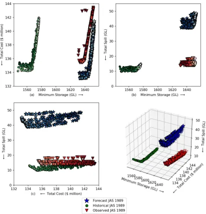
Figure 4: Average objective performance of Pareto sets from the forecast (stars), historical (circles), and observed (triangles) optimisation formulations for the July-September (JAS) 1989 historical planning period. The performance shown is that for that averaged over the forecast, historical, and observed inflow scenarios respectively.
difficult to determine the exact cause from this plot, the inflection point in the relationship between cost and minimum storage likely indicates options that result in the trigger of desalinated water production. The relationships between the three objectives for the case study and the decision variables have been elaborated further (for a 5-year assessment period) in Ashbolt et al. (2016b).
Figure 4 also illustrates the difference in objective performance when operating rules are optimised
according to the three different optimisation formulations, for the July-September 1989 planning period. The range in cost of the three Pareto sets are fairly similar, with slightly higher cost for the observed optimisation formulation. The historical optimisation formulation has lowest minimum system storage and spill (Figure 4 b). This is expected as it has the lowest total inflow (Table 5). Performance of the forecast-optimised Pareto set is most similar to the observed-optimised set for the objective trade-off curve of minimum storage and total cost (Figure 4 a). This is to be expected, as the average inflow of the forecast optimisation formulation is closest to the observed inflow (Table 5). However, the historical-optimised set is closer to the observed-optimised set in terms of spill (Figure 4 c). The reason for relatively low spill in the observed optimisation formulation, despite having higher total inflow volume (Table 5) than the forecast-optimised Pareto set, is less clear. A possible reason is a greater use of two-way pipelines, which can keep minimum storage higher but reduce spill by balancing water storages Ashbolt et al. (2016b). Another key difference between the observed optimisation formulation and the other two formulation is that operating rules are optimised to maximise performance for a single inflow condition, rather than average performance across five inflow scenarios. This may allow the operating rules to be 'more optimal' for the narrower range of inflow conditions. Similar behaviour was seen for the three other planning periods, with differences in relative performance due to the differences in forecast, historic, and observed inflows.
Operating rules
example, decision variable I, which governs the operation of the EPI two-way pipeline. However, the
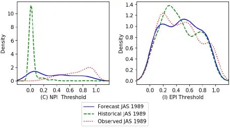
historical-optimised Pareto set shows significant difference to the other two sets in the distribution of decision variable C, which governs the direction of the NPI two-way pipeline. These figures suggest, for example, that the direction of the NPI two-way pipeline is switched more frequently (at lower thresholds) for the historic optimisation formulation than for the forecast and observed optimisation formulations, to avoid spills from storages or direct water to relatively water-scarce catchments. Overall, the distributions of the forecast-optimised set are similar to the observed set.
Figure 5: Distributions of decision variables C (NPI direction) and I (EPI direction) for July-September 1989 forecast, historical, and observed optimised scenarios, as kernel density estimation plots. Plots for all the decision variables A-P are shown in Figure S2.
Objective performance under observed conditions
Figure 4 showed the objective performance of three Pareto sets for July-September 1989, each of which were optimised and assessed to different average inflow conditions as outlined in Table 5. Based on such a figure, one Pareto set cannot be said to outperform another, since performance is dependent on different inflow volumes. Instead, simulating the performance of the forecast- and historical-optimised Pareto sets using the observed inflow for each planning period will allow a direct comparison of the Pareto sets and an idea of their performance as implemented over the planning period.
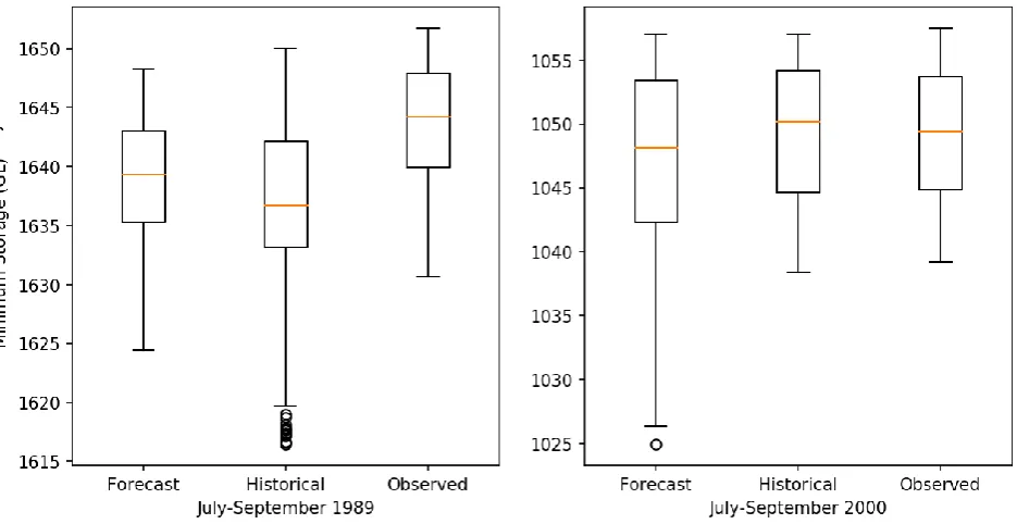
observed flow, for each of the four retrospective planning periods. These plots indicate the differences in distribution of objective performance between the three Pareto sets, indicated by the median (bar), box (25th – 75th percentile) and whiskers (minimum to maximum). Whilst there is significant overlap in the objective performance range, the differences between distributions of the optimisation formulations vary between planning periods. An example of the boxplot distributions of the minimum system storage objective for the July-September 1989 and 2000 planning periods is shown in Figure 6. For the July-September 1989 planning period, the median and range of minimum storage is most similar between the forecast- and observed-optimised Pareto sets. This is expected, since median forecast inflow was closer to observed flow than the historic median. For the July-September 2000 planning period, the historical-optimised Pareto set has more similar minimum system storage to the observed. This period had lower accuracy in the forecast, with observed inflow lower than but closest to the historic median.
Figure 6: Boxplots of minimum storage objective performance of the forecast-, historical- and observed-optimised Pareto sets for the July-September 1989 and 2000 planning periods, simulated using the observed inflow data for each period. Each box and whisker plot indicates the distribution and range of the 200+ operating options within each Pareto set, with the boxes indicating 25th-75th percentiles, bars indicating 50th
percentiles, and whiskers indicating minimum and maximum values.
Optimality under observed conditions
compare performance of operating options across all three objectives simultaneously. This comparison is important, as multi-objective optimisation is characterised by trade-offs between objectives and aims to find operating options that outperform others on all three objectives, i.e. are non-dominated. Whilst the three Pareto sets were non-dominated in terms of all three objectives for the optimised inflow, the objective performance of the forecast- and historical-optimised Pareto sets changed when simulated for observed inflow conditions. This means that the operating options may no longer be non-dominated under observed inflow conditions. The observed-optimised set, on the other hand, will remain non-dominated as it was optimised to observed inflow.
The proportion of non-dominated operating options within the forecast- and historical-optimised Pareto sets were reassessed using the observed inflow. This can be used as a measure of the relative optimality of the operating options resulting from the two optimisation formulations for the four different planning periods. The percentage of non-dominated operating options in each optimisation is shown in Table 6. This table indicates that for three of the four planning periods, there are a greater percentage of non-dominated operating options in the forecast-optimised Pareto sets. The difference is greatest for the July-September 1989 planning period, which had relatively high accuracy and was the only planning period with observed flow higher than forecast inflow. The July-September 2000 planning period had a higher number of
non-dominated forecast-optimised operating options, despite the historical median being closer to the observed flow. The July-September 1991 planning period, which had lowest accuracy in the forecast, had a slightly higher percentage of non-dominated operating options for the historical-optimised Pareto set. These results indicate that the forecast optimisation formulation provided benefits over the use of the historical optimisation formulation for most of the planning periods. Despite this, the differences between the historical optimisation formulation were relatively small for 3 of the 4 planning periods. This suggests that the benefits of using multiple inflow scenarios have mitigated some of the risk in observed inflow deviating from both the forecast- or historical-median.
Comparison of options selected using compromise programming
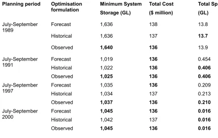
Table 7 shows the objective performance of the most efficient operating options from each of the three Pareto sets for each of the four planning periods, simulated for observed inflow conditions and using a preference of 30% weighting on minimum system storage, 40% on total cost, and 30% on total spill. This table shows that whilst some options have equal performance, none of the operating options outperforms all the others. Generally, the observed optimisation formulation has the best performance, which is equalled by the forecast-optimised option for the July-September 2000 period. The forecast-optimised option outperforms the historical-optimised option for the July-September 1997 and 2000 planning periods. However, the
historical-optimised option equals or improves on the forecast-optimised option for the July-September 1991 period. There is most similarity in cost between the options, perhaps due to the higher weighting on this objective. Overall, the forecast-optimised options perform better than the historical-optimised options, and similarly to the observed-optimised options. However the historical-optimised options also perform reasonably well, and there is often a relatively small difference between options.
Sensitivity analysis
Comparing the objective performance of operating options using the optimised inflow and observed inflow (e.g. Figures 4 and 6) suggested that the objective performance is significantly influenced by the total inflow volume. To understand how changes in the inflow volume affect the objective performance, the forecast-optimised Pareto set for July-September 1989 was also simulated using the 10th, 25th, 50th, 75th, and 90th
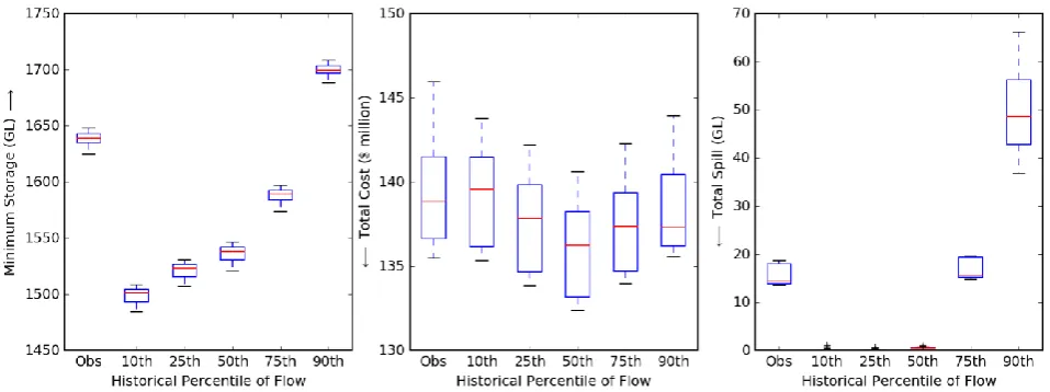
percentile historical inflow scenarios. Figure 7 shows boxplots of the sensitivity of objective performance of the forecast-optimised Pareto set for July-September 1989 to different inflow possibilities, including the observed inflow. These figures indicate that the both the minimum storage and total spill increase significantly with total inflow volume, to a degree much larger than the differences between optimisation formulations seen in Figure 6. The total cost on the other hand, is fairly similar across the different percentile flow scenarios, with lower cost incurred for 50th and 75th percentile flows. Overall, the minimum storage and
Figure 7: Performance of forecast-optimised Pareto set for July-September 1989, simulated using observed (obs) flow, and different percentile scenarios of inflow from the historical distribution of the July-September season.
The results also indicate that objective performance under observed inflow is sensitive to the inflow volume used in optimisation. Figure 8 compares the performance of the observed (obs.) and forecast-optimised (multi-forecast) Pareto sets July-September 1989, shown previously in Figure 6 and Figure S3, to Pareto sets optimised using single forecast 10th, 50th and 90th percentile inflow scenarios for the period. The
performance shown is that under observed inflow conditions, which for this planning period, was between the 50th and 75th percentile forecast inflows. These plots indicate that the observed and multi-scenario
forecast-optimised Pareto sets provide better results in terms of minimum storage and spill. Whilst the forecast 10th
and 90th percentile optimised Pareto sets have lower median cost, this comes at a trade-off for lower
minimum storage or higher spill. The 10th percentile scenario experiences significantly higher spill as it was
optimised to a much lower inflow volume than observed. The 90th percentile scenario experiences
significantly lower spill as it was optimised for higher flow conditions than observed, but the minimum storage is significantly lower. These plots indicate the importance of considering multiple inflow scenarios in
Figure 8: Objective performance of Pareto sets for July-September 1989, optimised to different scenarios of inflow: observed (Obs), averaged across multiple inflows (10, 25th, 50th, 75th and 90th) (Multiforecast), 10th
percentile forecast inflow (Forecast 10th), 50th percentile forecast inflow (Forecast 50th), and 90th percentile
forecast inflow (Forecast 90th). For this time period, total observed inflow was between the volumes of the 50th and 75th inflow scenarios.
Summary and conclusions
In summary, this study has shown how including streamflow forecast information in short-term operational planning for water grids has the potential to improve multi-objective performance of operating rules. This improvement was measured as a positive change in objective performance compared to operating rules optimised to inflows from the historical distribution. This was demonstrated for a case study water grid, for four retrospective (past) three-month planning periods, by optimising operating rules to meet multiple management objectives – maximising water security, minimising operational cost, and minimising spill volumes – averaged across multiple scenarios of historically-sampled inflow. Forecast-optimised Pareto sets of operating options were identified by optimising operating rules for inflow scenarios sampled from historical inflow based on publicly-available forecast probabilities.
On average, the forecast-optimised operating options presented in this study improved objective
climatology. This would be aided by additional measures of forecast skill that could provide a more robust assessment of forecast value for decisionmakers (see Anghileri et al. 2006, Watkins & Wei 2008).
Despite the simplicity of the method used in this study for translating streamflow forecast information, the results indicated potential improvements in objective performance. The relatively good performance of the forecast-optimised set across all planning periods suggests that using forecast information, with multiple scenarios of inflow, may provide an acceptable trade-off between the benefits and risks of forecast accuracy. The use of multiple inflow scenarios in particular appears to provide benefits in managing inflow risk
compared to a single scenario of inflow, even when the forecast is relatively accurate. This suggests that available forecast information (such as that provided by the Bureau of Meteorology in Australia) can be used to improve existing model inputs with relatively little investment, by simply updating the distribution of sampled inflow to reflect current and expected conditions. Nevertheless, further assessment by decisionmakers is recommended when applying this method to additional case studies and planning seasons, to verify these benefits and the acceptable risk vs reward ratio.
This paper has used a relatively simple method to translate publicly-available streamflow forecast information to inflow timeseries at 39 inflow nodes in the case study simulation-optimisation model, using currently available data. This simplification was required since forecast inflow timeseries were unavailable at locations corresponding to the model inflow sites. Instead, the flow duration curves, representing the inflow
distributions, were used to translate available streamflow forecast volumes at forecast sites to inflow volumes at nearby (highly correlated) case study model inflow sites. Whilst this method preserved sub-seasonal cross-correlation within basin groups, only seasonal volumes were correlated across basin groups. A potential improvement in spatial correlation of streamflow forecasts at each of the model sites could be obtained using spatial reconstruction methods such as those applied to climate forecasts by Verkade et al. (2013), Voisin et al. (2010) and Wood & Lettenmaier (2006). Additional measures of forecast quality presented by Bradley et al. (2003) would assist in assessing the correlation between historical or forecast inflow at the available forecast sites and the observations at each of the model inflow sites.
Improvements to the robustness of operating rules could be made by developing stochastic catchment models that incorporate variability in the daily patterns of flow and to generate inflow patterns more consistent with initial catchment condition and season. Alternatively, methods for generating forecast
increase robustness to both different inflow volumes and different sequencing of the total inflow volume over the time period. This is important, since the pattern of flow may affect the operating rules and objective performance (Faber and Stedinger 2001).
This study has also shown the potential utility of the forecasts provided by the Bureau of Meteorology to short-term operational planning in Australia. The more recent forecasts by the Bureau of Meterology provide seasonal volumes with a monthly timestep; improving the method presented here to incorporate this monthly pattern may reduce the uncertainty in the timing of intra-seasonal flow. Current plans to extend the 3 month forecasts to 1 year (Wang et al. 2014) should allow the operating rules to be optimised for expected inflows over the entire annual operational planning period for the case study. An alternative is to develop a method for extending the 3-month streamflow sequences, preferably one that preserves serial correlation (Watkins et al. 2000). The simulation-optimisation process may still be repeated on a monthly or seasonal basis, since the forecasts are more accurate for the first 3 months (Simonovic and Burn 1989; Wang et al. 2014).
Finally, a sensitivity assessment of objective performance to total inflow indicated that for some of the case study objectives (minimum storage and spill), performance was more sensitive to the inflows experienced during the planning period than the operating rules themselves. Conversely, another objective (total cost) was less sensitive to observed inflow. Thus it is important for the decision-maker to simulate the performance of the Pareto set or chosen operating options under a range of inflow conditions to understand the sensitivity of different objectives to the observed inflow or to the optimised operating rules. This may aid the
optimisation problem formulation and identify critical measures of robustness.
In conclusion, the previous study (Ashbolt et al. 2016a) showed how multi-objective optimisation of annual operating rules using historical inflow can provide improvements to objective performance compared to rules-based operation using longer-term operating rules. This study builds on that study by showing how
Acknowledgements
The authors wish to acknowledge the assistance of anonymous reviewers in improving the manuscript. They also wish to acknowledge Seqwater in providing input data for the simulation-optimisation model and QJ Wang for providing information on streamflow forecasts.
Supplemental Data
References
Alemu ET (2011) Decision Support System for Optimizing Reservoir Operations Using Ensemble Streamflow Predictions. J Water Resour Plan Manag 137:72.
Anghileri, D. et al., 2016. Value of long-term streamflow forecasts to reservoir operations for water supply in snow-dominated river catchments. Water Resources Research, 52(6), pp.4209–4225. Available at: http://dx.doi.org/10.1002/2015WR017864.
Archfield SA, Vogel RM (2010) Map correlation method: Selection of a reference streamgage to estimate daily streamflow at ungaged catchments. Water Resour Res 46:1–15. doi: 10.1029/2009WR008481 Ashbolt S, Maheepala S, Perera BJC (2016a) Using Multiobjective Optimization to Find Optimal Operating
Rules for Short-Term Planning of Water Grids. J Water Resour Plan Manag 142:4016033. doi: 10.1061/(ASCE)WR.1943-5452.0000675
Ashbolt S, Maheepala S, Perera BJC (2014) A Framework for Short-term Operational Planning for Water Grids. Water Resour Manag 28:2367–2380. doi: 10.1007/s11269-014-0620-4
Ashbolt SC, Maheepala S, Perera BJC (2016b) Interpreting a Pareto set of operating options for water grids: a framework and case study. Submitt to Hydrol Sci J 1–43.
Australian Government Bureau of Meteorology. (2017) "Seasonal Streamflow Forecasts." <http://www.bom.gov.au/water/ssf/forecasts.shtml>, (Nov. 12 2017)
Ballestero E (2007) Compromise programming: A utility-based linear-quadratic composite metric from the trade-off between achievement and balanced (non-corner) solutions. Eur J Oper Res 182:1369–1382. doi: http://dx.doi.org/10.1016/j.ejor.2006.09.049
Beh EHY, Maier HR, Dandy GC (2015) Scenario driven optimal sequencing under deep uncertainty. Environ Model Softw 68:181–195. doi: http://dx.doi.org/10.1016/j.envsoft.2015.02.006
Bradley, A., Hashino, T. & Schwartz, S., 2003. Distributions-Oriented Verification of Probability Forecasts for Small Data Samples. Weather and Forecasting, 18, pp.903–917.
Brown CM, Lund JR, Cai X, Reed PM, Zagona EA, Ostfeld A, Hall J, Characklis GW, Yu W, Brekke L (2015) The future of water resources systems analysis: Toward a scientific framework for sustainable water management. Water Resour Res 51:6110–6124. doi: 10.1002/2015WR017114
Clark M, Gangopadhyay S, Hay L, Rajagopalan B, Wilby R (2004) The Schaake Shuffle: A Method for Reconstructing Space–Time Variability in Forecasted Precipitation and Temperature Fields. J Hydrometeorol 5:243–262. doi: 10.1175/1525-7541(2004)005<0243:TSSAMF>2.0.CO;2
Deb K, Pratap A, Agarwal S, Meyarivan T (2002) A Fast and Elitist Multiobjective Genetic Algorithm: NSGA-II. IEEE Trans Evol Comput 6:182–197.
Dutta D, Wilson K, Welsh WD, Nicholls D, Kim S, Cetin L (2013) A new river system modelling tool for sustainable operational management of water resources. J Environ Manage 121:13–28. doi: http://dx.doi.org/10.1016/j.jenvman.2013.02.028
Faber BA, Stedinger JR (2001) Reservoir optimization using sampling SDP with ensemble streamflow prediction (ESP) forecasts. J Hydrol 249:113–133.
Gelati E, Madsen H, Rosbjerg D (2013) Reservoir operation using El Niño forecasts—case study of Daule Peripa and Baba, Ecuador. Hydrol Sci J 59:1559–1581. doi: 10.1080/02626667.2013.831978 Georgakakos KP, Graham NE (2008) Potential Benefits of Seasonal Inflow Prediction Uncertainty for
decision-making under climate change. Clim Change 1–16. doi: 10.1007/s10584-015-1586-9 Gong G, Wang L, Condon L, Shearman A, Lall U (2010) A Simple Framework for Incorporating Seasonal
Streamflow Forecasts into Existing Water Resource Management Practices1. JAWRA J Am Water Resour Assoc 46:574–585. doi: 10.1111/j.1752-1688.2010.00435.x
Harrison B, Bales R (2016) Skill Assessment of Water Supply Forecasts for Western Sierra Nevada Watersheds. J Hydrol Eng 4016002. doi: 10.1061/(ASCE)HE.1943-5584.0001327
Higgins A, Archer A, Hajkowicz S (2008) A Stochastic Non-linear Programming Model for a Multi-period Water Resource Allocation with Multiple Objectives. Water Resour Manag 22:1445–1460.
Kim J-H (2008) Single-reservoir operating rules for a year using multiobjective genetic algorithm. J Hydroinformatics 10:163–179.
Krzysztofowicz R (2001) The case for probabilistic forecasting in hydrology. J Hydrol 249:2–9. doi: 10.1016/s0022-1694(01)00420-6
Kumar DN, Lall U, Petersen MR (2000) Multisite disaggregation of monthly to daily streamflow. Water Resour Res 36:1823–1833. doi: 10.1029/2000WR900049
Kumphon B (2013) Genetic Algorithms for Multi-objective Optimization: Application to a Multi-reservoir System in the Chi River Basin, Thailand. Water Resour Manag 27:4369–4378. doi: 10.1007/s11269-013-0416-y
Lee T, Salas JD, Prairie J (2010) An enhanced nonparametric streamflow disaggregation model with genetic algorithm. Water Resour Res 46:n/a--n/a. doi: 10.1029/2009WR007761
Li W, Sankarasubramanian A, Ranjithan RS, Brill ED (2014) Improved regional water management utilizing climate forecasts: An interbasin transfer model with a risk management framework. Water Resour Res. doi: 10.1002/2013WR015248
Maier HR, Guillaume JHA, van Delden H, Riddell GA, Haasnoot M, Kwakkel JH (2016) An uncertain future, deep uncertainty, scenarios, robustness and adaptation: How do they fit together? Environ Model Softw 81:154–164. doi: http://dx.doi.org/10.1016/j.envsoft.2016.03.014
Maier HR, Kapelan Z, Kasprzyk J, Kollat J, Matott LS, Cunha MC, Dandy GC, Gibbs MS, Keedwell E, Marchi A, Ostfeld A, Savic D, Solomatine DP, Vrugt JA, Zecchin AC, Minsker BS, Barbour EJ, Kuczera G, Pasha F, Castelletti A, Giuliani M, Reed PM (2014) Evolutionary algorithms and other metaheuristics in water resources: Current status, research challenges and future directions. Environ Model Softw 62:271–299. doi: http://dx.doi.org/10.1016/j.envsoft.2014.09.013
Mortazavi-Naeini M, Kuczera G, Kiem AS, Cui L, Henley B, Berghout B, Turner E (2015) Robust optimization to secure urban bulk water supply against extreme drought and uncertain climate change. Environ Model Softw 69:437–451. doi: http://dx.doi.org/10.1016/j.envsoft.2015.02.021
National Oceanic and Atmospheric Administration (2016) NOAA - National Weather Service - Water. http://water.weather.gov/ahps/forecasts.php. Accessed 20 Jun 2006
Pagano TC, Hartmann HC, Sorooshian S (2002) Factors affecting seasonal forecast use in Arizona water management: A case study of the 1997-98 El Niño. Clim Res 21:259–269.
Piechota T, Chiew F, Dracup J, McMahon T (2001) Development of Exceedance Probability Streamflow Forecast. J Hydrol Eng 6:20–28. doi: 10.1061/(ASCE)1084-0699(2001)6:1(20)
Ray P, Watkins D, Vogel R, Kirshen P (2014) A Performance-Based Evaluation of an Improved Robust Optimization Formulation. J Water Resour Plan Manag 140:4014006. doi: 10.1061/(ASCE)WR.1943-5452.0000389
of Hydrology, 497, pp.80–96. Available at:
http://www.sciencedirect.com/science/article/pii/S0022169413003958.
Robertson DE, Wang QJ (2009) Selecting predictors for seasonal streamflow predictions using a Bayesian joint probability (BJP) modelling approach. 18th World IMACS Congr. MODSIM09 Int. Congr. Model. Simul.
Sankarasubramanian A, Lall U, Devineni N, Espinueva S (2009a) The role of monthly updated climate forecasts in improving intraseasonal water allocation. J Appl Meteorol Climatol 48:1464–1482. doi: 10.1175/2009jamc2122.110.1029/2002WR001373
Sankarasubramanian A, Lall U, Souza Filho FA, Sharma A (2009b) Improved water allocation utilizing probabilistic climate forecasts: Short-term water contracts in a risk management framework. Water Resour Res 45:n/a-n/a. doi: 10.1029/2009WR007821
Seqwater (2014) Annual Operations Plan – May 2014. Brisbane, Australia
Simonovic SP, Burn DH (1989) An improved methodology for short-term operation of a single multipurpose reservoir. Water Resour Res 25:1–8. doi: 10.1029/WR025i001p00001
Verkade, J.S. et al., 2013. Post-processing ECMWF precipitation and temperature ensemble reforecasts for operational hydrologic forecasting at various spatial scales. Journal of Hydrology, 501(0), pp.73–91. Available at: http://www.sciencedirect.com/science/article/pii/S0022169413005660.
Voisin, N., Schaake, J.C. & Lettenmaier, D.P., 2010. Calibration and Downscaling Methods for Quantitative Ensemble Precipitation Forecasts. Weather and Forecasting, 25(6), pp.1603–1627. Available at: http://dx.doi.org/10.1175/2010WAF2222367.1.
Walker EW, Haasnoot M, Kwakkel HJ (2013) Adapt or Perish: A Review of Planning Approaches for Adaptation under Deep Uncertainty. Sustainability. doi: 10.3390/su5030955
Wang E, Zhang Y, Luo J, Chiew FHS, Wang QJ (2011) Monthly and seasonal streamflow forecasts using rainfall-runoff modeling and historical weather data. Water Resour Res 47:W05516. doi:
10.1029/2010WR009922
Wang QJ, Bennett J, Schepen A, Robertson D, Song Y, Li M (2014) Ensemble Forecasting Of Seasonal Streamflow Using Climate Forecasts as Inputs. APEC Clim. Symp. APEC Climate Center, Nanjing, China, pp 11–12
Wang QJ, Robertson DE (2011) Multisite probabilistic forecasting of seasonal flows for streams with zero value occurrences. Water Resour Res 47:W02546. doi: 10.1029/2010wr009333
Wang QJ, Robertson DE, Chiew FHS (2009) A Bayesian joint probability modeling approach for seasonal forecasting of streamflows at multiple sites. Water Resour Res 45:W05407. doi:
10.1029/2008wr007355
Watkins DW, McKinney DC, Lasdon LS, Nielsen SS, Martin QW (2000) A scenario-based stochastic programming model for water supplies from the highland lakes. Int Trans Oper Res 7:211–230. doi: 10.1111/j.1475-3995.2000.tb00195.x
Watkins, D.W. & Wei, W., 2008. The value of seasonal climate forecasts and why water managers don’t use them. World Environmental and Water Resources Congress 2008, 316. Available at:
http://www.scopus.com/inward/record.url?eid=2-s2.0-79251475589&partnerID=40&md5=2792fc7bd0d4adb23862e999167617dc.
Whateley, S., Palmer, R.N. & Brown, C., 2015. Seasonal hydroclimatic forecasts as innovations and the challenges of adoption by water managers. Journal of Water Resources Planning and Management, 141(5). Available at:
Wood, A.W. & Lettenmaier, D.P., 2006. A Test Bed for New Seasonal Hydrologic Forecasting Approaches in the Western United States. Bulletin of the American Meteorological Society, 87(12), pp.1699–1712. Available at: http://dx.doi.org/10.1175/BAMS-87-12-1699.
Wu, L. et al., 2011. Generation of ensemble precipitation forecast from single-valued quantitative
precipitation forecast for hydrologic ensemble prediction. Journal of Hydrology, 399(3–4), pp.281–298. Available at: http://www.sciencedirect.com/science/article/pii/S0022169411000382.
Zeleny M (1973) Compromise programming, multiple criteria decision-making. In: Cochrane JL, Zeleny M (eds) Mult. Criteria Decis. Mak. University of South Carolina Press, Columbia, pp 263–301
Table 1: List of model catchment groups for the case study, including four Bureau of Meterology (BoM) forecast sites, model catchment group representatives, and model catchments within the catchment group.
Group BoM forecast site Model catchment group representative
Model catchments within group
1 Back Creek at Beachmont Little Nerang Dam Inflow Gold Coast, Redlands 2 Burnett Creek upstream of Maroon
Dam
Maroon Dam Inflow Bremer, Logan
3 Tinana Creek at Tagigan Road Lake MacDonald Downstream Inflow
Caboolture, Mary, Maroochy, Mooloolah