MRI Image Sample Noise Filtration and a Design Toolbox to Generate Complex Phantoms in Medical Image Processing

(1)

International Journal of Computer Science and Mobile Computing

A Monthly Journal of Computer Science and Information Technology

ISSN 2320–088X

IJCSMC, Vol. 2, Issue. 12, December 2013, pg.254 – 265

RESEARCH ARTICLE

MRI Image Sample Noise Filtration and

a Design Toolbox to Generate Complex

Phantoms in Medical Image Processing

Arya Ghosh1, Himadri Nath Moulick2, Priyanka Das3

¹CSE & West Bengal University of Technology, India ²CSE & West Bengal University of Technology, India ³CSE & West Bengal University of Technology, India 1

[email protected]; 2 [email protected]; [email protected]

Abstract— In this paper a modified spatial filtration approach is suggested for image de-noising applications. The existing spatial filtration techniques were improved for the ability to reconstruct noise-affected medical images. The developed modified approach is developed to adaptively decide the masking centre for a given MRI image. The conventional filtration techniques using mean, median and spatial median filters were analysed for the improvement in modified approach. The developed approach is compared with current image smoothening techniques. The proposed approach is observed to be more accurate in reconstruction over other conventional techniques. In the field of medical image processing, the evaluation of new algorithms is often a difficult task since real data sets do not allow a quantitative evaluation of the algorithms’ properties and the correctness of results. Thus, a phantom design toolbox was developed to enable the generation of complex geometries appropriate to simulate anatomical structures as well as realistic image intensity properties and artefacts, such as noise and in homogeneities. This paper describes the most important features of the new toolbox and shows sample phantoms generated so far.

Keywords— Spatial Filter; Image De-noising; Modified Spatial Filter; RMSE; Image Smoothening

I. INTRODUCTION

(2)

(3)

The simplest of smoothing algorithms is the Mean Filter. Mean filtering is a simple, intuitive and easy to implement method of smoothing medical images, i.e. reducing the amount of intensity variation between one pixel and the next. It is often used to reduce noise in MRI images. The idea of mean filtering is simply to replace each pixel value in an image with the mean (‘average’) value of its neighbours, including itself. This has the effect of eliminating pixel values, which are unrepresentative of their surroundings. The mean value is defined by,

……….(1) Where, N : number of pixels

xi : corresponding pixel value,

I : 1….. N.

The mean filtration technique is observed to be lower in maintaining edges within the images. To improve this limitation a median filtration technique is developed. The median filter is a non-linear digital filtering technique, often used to remove noise from medical images or other signals. Median filtering is a common step in image processing. It is particularly useful to reduce speckle noise and salt and pepper noise. Its edge preserving nature makes it useful in cases where edge blurring is undesirable. The idea is to calculate the median of neighbouring pixels’ values. This can be done by repeating these steps for each pixel in the medical image.

a) Store the neighbouring pixels in an array. The neighbouring pixels can be chosen by any kind of

shape, for example a box or a cross. The array is called the window, and it should be odd sized.

b) Sort the window in numerical order

c) Pick the median from the window as the pixels value. The median is defined by,

……….………..(2)

where, i = 1…. N. These filtration techniques were found to be effective in gray scale images. When processed over color images these filtration techniques give lesser performance. To achieve accurate reconstruction of medical image the median filtration technique is modified to spatial median filtration. The Spatial Median Filter is a uniform smoothing algorithm with the purpose of removing noise and fine points of medical image data while maintaining edges around larger shapes. The basic algorithm for spatial median filter is as outlined below, the algorithm determines the Spatial Median of a set of points, x1, ...,xN :

1. For each vector x, compute S, which is a set of the sum of the spatial depths from x to every other vector.

2. Find the maximum spatial depth of this set, Smax

3. Smax is the Spatial Median of the set of points. The spatial depth between a point and set of

points is defined by,

….…..…(3)

(4)

A. Modified Spatial Filter

In a Spatial Median Filter the vectors are ranked by some criteria and the top ranking point is used to the replace the centre point. No consideration is made to determine if that centre point is original data or not. The unfortunate drawback to using these filters is the smoothing that occurs uniformly across the image. Across areas where there is no noise, original medical image data is removed unnecessarily. In the Modified Spatial Median Filter, after the spatial depths between each point within the mask are computed, an attempt is made to use this information to first decide if the mask’s centre point is an uncorrupted point. If the determination is made that a point is not corrupted, then the point will not be changed. The proposed modified filtration works as explained below:

1) Calculate the spatial depth of every point within the mask selected. 2) Sort these spatial depths in descending order.

3) The point with the largest spatial depth represents the Spatial Median of the set. In cases where noise is determined to exist, this representative point is used to replace the point currently located under the canter of the mask.

4) The point with the smallest spatial depth will be considered the least similar point of the set.

5) By ranking these spatial depths in the set in descending order, a spatial order statistic of depth

levels is created.

6) The largest depth measures, which represent the collection of uncorrupted points, are pushed to the front of the ordered set.

7) The smallest depth measures, representing points with the largest spatial difference among others in the mask and possibly the most corrupted points, and they are pushed to the end of the list.

This prevents the smoothing by looking for the position of the centre point in the spatial order

statistic list. For a given parameter ( where mask size) which represents the estimated number of original points under a mask of points. As stated earlier, points with high spatial depths are at the beginning of the list. Pixels with low spatial depths appear at the end.

If centre point then current pixel MSF

else if centre point then current pixel MSF

else if then, pixel cannot be modified. If the position of the centre mask point appears

within the first bins of the spatial order statistic list, then the centre point is not the best representative point of the mask, and it is still original data and should not be replaced. Two things should be noted about the use ofin this approach. When is 1, this is the equivalent

to the unmodified Spatial Median Filter. When is equal to the size of the mask, the canter

(5)

III.SYSTEM DESCRIPTION

The toolbox is provided with a graphical user interface based on Qt 4.5 [6] to easily choose, transform and combine geometrical primitives based on constructive solid geometry (CSG) [17]. Three orthogonal 2D views and one 3D view enable the user to monitor the phantom building process step-by-step.

A. Available Primitives

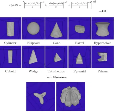
So far, various rotationally symmetric and polygonal 2D and 3D primitives, as shown in Fig. 1, are available. In addition to these simple geometric primitives, a primitive called three dimensional super shape is made available. This primitive is based on the “Super formula” introduced by Gielis [21] designed “to study natural forms and phenomena”. Besides known approaches to create 3D super shapes by extrusion and the spherical product [9], a new approach is made available (1), (Fig. 2).

…(4)

Fig. 1. 3D primitives.

(6)

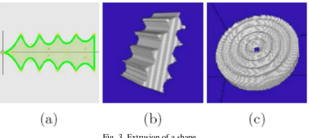
Fig. 3. Extrusion of a shape.

In order to generate even more complex and freely definable primitives, the toolbox provides a tool to draw two-dimensional boundary contours based on linear, quadratic and Bezier curves. The vowelised two-dimensional object (Fig. 3(a)) can then be extruded in one direction (Fig. 3(b)) or around one axis (Fig. 3(c)).

B. Composition of Phantoms

The primitives chosen can be defined in value, size and position and be transformed by affine transformations. The boundary representation of the primitives is used to transform and position them on the volume grid. Phantoms can be composed of primitives using the Boolean operations union, difference, intersect or distinguish. The intensity value of the resulting combination can be calculated from the input values by operations, such as sum, difference or product. The resulting combination can in turn be used like a single primitive in further steps and be integrated into a user specific library. In addition, the discrete values of the components can be modified to simulate real images including definable image artefacts, such as additive white Gaussian noise, and different kinds of in homogeneities, such as nonlinear intensity non-uniformity fields from estimated real MRI scans [14]. In order to separate a phantom into different tissue types (e.g., white and grey matter for brain phantoms) dependent on the distance to the phantom’s surface, an operation based on a distance transformation is made available. The phantoms can be saved in all possible big and little raw data formats and different file formats, e.g., RAW and Analyse 7.5. The phantom exports module allows further histogram-based modifications of already assigned values, e.g., clipping or histogram equalization. Furthermore, the whole phantom building process can be saved in an editable XML file, to enable the user to stop and rebuild or modify the phantom at each step of the building procedure.

IV.RESULTS AND DISCUSSIONS

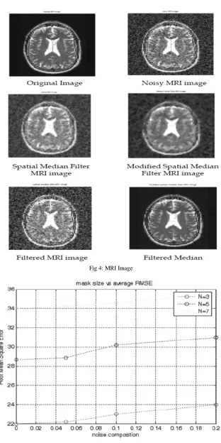
Different stages of filtered MRI images are shown in Fig.4. To test the accuracy of the modified spatial median filter, a medical image with corruption applied by some means is applied. To estimate the quality of a reconstructed MRI image, first calculate the Root-Mean- Squared Error between the original and the reconstructed image. The Root-Mean-Squared Error (RMSE) for an original image I and reconstructed MRI image R is defined by,

(7)

(8)

Fig 4: MRI Image

(9)

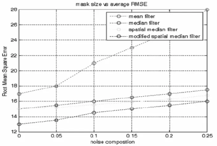
Fig 6: Effectiveness of Noise Filters for Various Noise Compositions

(10)

Fig. 7. Graphical User Interface

(11)

Fig. 9. The phantom (right) is derived from a sample slice of the brain [11] (left).

V. CONCLUSIONS

This paper introduces two new filters for removing impulse noise from images and shown how they compare to other well-known techniques for noise removal. First, common noise filtering algorithms were discussed. Next, a Spatial Median Filter was proposed based on a combination of work on the Median Filter and the Spatial Median quantile order statistic. Seeing that the order statistic could be utilized in order to make a judgment as to whether a point in the signal is considered noise or not, a Modified Spatial Median Statistic is proposed. The Modified Spatial Median Filter requires two parameters: A window size and a threshold T of the estimated non-noisy pixels under a mask. In the results, the best threshold T to use in the Modified Spatial Median Filter and determined that the best threshold is 4 when using a 3×3 window m ask size. Using these as parameters, this filter was included in a comparison of the Mean, Median, and Spatial Median Noise Filters. In the broad comparison of noise removal filters, it was concluded that for images containing p = 0.15 noise composition, the Modified Spatial Median Filter performed the best and that the Component Median Filter performed the best overall noise models tested. Simulating complex geometries of anatomical regions is a difficult and time consuming task. The phantom design toolbox allows building such complex phantoms in a fast, intuitive and easy way. Pairs of realistic-looking phantoms, one representing the anatomical structures and one representing the corresponding gray value image (e.g., of a simulated MR dataset), can be created to evaluate medical image processing algorithms. A second toolbox is already implemented to enable those quantitative evaluations.

REFERENCES

[1] R. Hodgson, D. Bailey, M. Naylor, A. Ng, and S. McCNeil, “Properties, Implementations and Applications of Rank filters”, Image Vision Comput., 3, pp. 3–14, 1985.

[2] M. Cree, “Observations on Adaptive Vector Filters for Noise Reduction in Color Images”, IEEE Signal ProcessingLetters, 11, No. 2, pp. 140–143, 2004.

[3] P. Lambert and L. Macaire, “Filtering and Segmentation: The Specificity of Color Images”, Proc. Conference on Colorin Graphics and Image Processing, Saint-Etienne.

[4] I. Pitas and P. Tsakalides, “Multivariate Ordering in Color Image Filtering”, IEEE Transactions on Circuits and Systems for Video Technology, 1, pp. 247–259, 1991.

[5] R. Lukac, B. Smolka, K. Plataniotis, and A. Venetsanopoulos, “Selection Weighted Vector Directionnal Filters”, Computer Vision and Image Understanding, 94, pp. 140–167, 2004.

[6] M. Vardavoulia, I. Andreadis, and P. Tsalides, “A New Median Filter for Colour Image Processing”,

PatternRecognition Letters, 22, pp. 675–689, 2001.

[7] A. Koschan and M. Abidi, “A Comparison of Median Filter Techniques for Noise Removal in Color Images”, Proc. 7th German Workshop on Color Image Processing, 34, No. 15, pp. 69–79, 2001.

[8] R. Lukac, “Adaptive Vector Median Filtering”, Pattern Recognition Letters, 24, pp. 1889–1899, 2002. [9] L. Khriji and M. Gabbouj, “Vector Medianrational Hybrid Filters for Multichannel Image Processing”,

(12)

[10] Raymond H. Chan, Chung-Wa Ho, and Mila Nikolova, “Salt-and-Pepper Noise Removal by Median-Type Noise Detectors and Detail-Preserving Regularization”, IEEE Trans. Image Processing, 14, No. 10, 2005. [11] K. S. Srinivasan and D. Ebenezer, “New Fast and Efficient Decision-Based Algorithm for Removal of

High-Density Impulse Noises”, IEEE Signal Processing Letters, 14, No. 3, 2007.

[12] Rabie, “Robust Estimation Approach for Blind Denoising”, IEEE Trans. Image Processing, 14, No.11, pp. 1755-1765, 2005.

[13] R. Kashyap and K. Eom, “Robust Image Modeling Techniques with an Image Restoration Application”, IEEE Trans. Acoust. Speech Signal Process, 36, No. 8, pp.1313-325, 1988.

[14] Wagenknecht G, Winter S. Volume-of-interest segmentation of cortical regions for multimodal brain analysis. Conf Record IEEE NSS/MIC. 2008; p. M06–455

[15] Kennedy DN, Worth AJ, Caviness VS. MRI-Based internet brain segmentation repository. Proc ISMRM. 1996;4(3):1657.

[16] Rex DA, Ma JQ, Toga AW. The LONI pipeline processing environment. Neuroimage.

[17] Cocosco CA, et al. BrainWeb: Online interface to a 3D MRI simulated brain database. NeuroImage. 1997;5(4):425..multimodal brain

[18] Hamo O, Nelles G, Wagenknecht G. A phantom design toolbox to generate simulated data suitable for the evaluation of segmentation algorithms. Proc IFMBE. 2009;25:PD 64.

[19] Qt 4.5: Qt‘s Classes. Nokia Corporation and/or its subsidiaries; 2009 [cited 2009 Aug 16]. Available from: URL: http://doc.trolltec.com/4.5/classes.

[20] Watt A. 3D-Computergrafik. vol. 3. Pearson Studium; 2003.

[21] Gielis J. A generic geometric transformation that unifies a wide range of natural and abstract shapes. American J of Botany. 2003;90(3):333–8.

[22] Bourke P. Supershape in 3D [Online]; 2003 [cited 2009 Okt 16]. Available from: URL:http:/local.wasp.uwa.edu.au/ pbourke/geometry/supershape3d/.

[23] Arcadian. Gray733. Wikipedia; 2007 [cited 2009 Okt 10]. Available from: URL: http://commons.wikimedia.org/wiki/File:Gray733.png.