Eleventh Floor, Menzies Building
Monash University, Wellington Road
C
LAYTONVic 3800 A
USTRALIAfrom overseas:
Telephone:
(03) 9905 2398, (03) 9905 5112
61 3 9905 2398 or
61 3 9905 5112
Fax:
(03) 9905 2426
61 3 9905 2426
e-mail:
[email protected]
Internet home page:
http//www.monash.edu.au/policy/
PHILGEM: A SAM-based
Computable General Equilibrium
Model of the Philippines
byErwin L. Corong and J. Mark Horridge
Centre of Policy Studies, Monash University
General Paper No. G-227 April 2012
ISSN 1 031 9034
ISBN 978 1 921654 35 0
PHILGEM: A SAM-based Computable
General Equilibrium Model of the
Philippines
Erwin L. Corong and J. Mark Horridge
1Centre of Policy Studies, Monash University, Australia
Abstract:This paper describes the structure of PHILGEM, a single country computable general equilibrium (CGE) model of the Philippine economy. PHILGEM offers a good starting point for model development, especially for researchers who may want to extend their ORANI-G models to draw on supplementary data coming from a social accounting matrix (SAM). A generic ver-sion of the model is described here designed for expository purposes and for adaptation to other countries. The description of PHILGEM's equations and database is closely integrated with an explanation of how the model is solved using the GEMPACK system. Computer files are freely available, which contain a complete model specification and database.
Bibliographical note: The PHILGEM model and its documentation draws from: Horridge, J.M. (2003) ORANI-G: A Generic Single-Country Computable General
Equilibrium Model, Centre of Policy Studies, Monash University.
Latest PHILGEM or ORANI-G related material will be found at: http://www.monash.edu.au/policy/oranig.htm
1
Contents
1. Introduction 1
2. Model Structure and Interpretation of Results 2
2.1. A comparative-static interpretation of model results 2
3. The Percentage-Change Approach to Model Solution 3
3.1. Levels and linearised systems compared: a small example 5
3.2. The initial solution 6
4. The Equations of PHILGEM 6
4.1. The TABLO language 7
4.2. The naming system 8
4.3. The model's data base 9
4.4. Dimensions of the model 15
4.5. Core data coefficients and related variables 17
4.6. The equation system 22
4.7. Structure of production 22
4.8. Demands for primary factors 23
4.9. Sourcing of intermediate inputs 26
4.10. Top production nest 28
4.11. Industry costs and production taxes 29
4.12. From industry outputs to commodity ouputs 30
4.13. Export and local market versions of each good 31
4.14. Demands for investment goods 32
4.15. Household demands 34
4.16. Export demands 38
4.17. Other final demands 40
4.18. Demands for margins 41
4.19. Formulae for sales aggregates 41
4.20. Market-clearing equations 42
4.21. Purchasers' prices 43
4.22. Indirect taxes 44
4.23. GDP from the income and expenditure sides 46
4.24. The trade balance and other aggregates 49
4.25. Primary factor aggregates 50
4.26. Rates of return and investment 51
4.27. The labour market 53
4.28. Miscellaneous equations 54
4.29. Adding variables for explaining results 54
4.30. Sales decomposition 55
4.31. The Fan decomposition 55
4.32. The expenditure side GDP decomposition 56
4.33. Checking the data 59
4.34. Summarizing the data 60
4.35. Import shares and short-run supply elasticities 61
4.36. Storing Data for Other Computations 62
5. Equations for SAM extension 64
5.1. Gross Operating Surplus 64
5.2. Enterprises Account 65
5.3. Labour income of households 67
5.4. Household income 69
5.5. Household consumption function, savings and other transfers 71
5.6. Government Income 71
5.8. Private investment expenditure 73
5.9. Rest of the world 74
5.10. SAM consistency 74
5.11. Revenue Neutrality 75
5.12. Household results for reporting purposes 79
5.13. Deriving a Macro SAM 76
5.14. Condensation 78
6. Closing the Model 81
7. Using GEMPACK to Solve the Model 85
8. Conclusion 87
References 88
Appendix A: Percentage-Change Equations of a CES Nest 89
Appendix B: PHILGEM on the Web 91
Appendix C: Hardware and Software Requirements for Using GEMPACK 91 Appendix D: Main differences between full-size PHILGEM and the version described here 92
Appendix E: Deriving Percentage-Change Forms 92
Appendix F: Algebra for the Linear Expenditure System 93
Appendix G: Making your own AGE model from PHILGEM 95
Appendix H: Formal Checks on Model Validity; Debugging Strategies 97
Appendix I: Short-Run Supply Elasticity 98
Appendix J: List of Variables 100
List of Figures
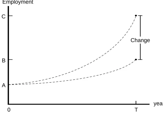
Figure 1. Comparative-static interpretation of results 2
Figure 2. Linearisation error 4
Figure 3. Multistep process to reduce linearisation error 4
Figure 4. The PHILGEM Flows Database 10
Figure 5. PHILGEM Aggregate Social Accounting Matrix (SAM) Database 12
Figure 6. PHILGEM Aggregate SAM (in millions of pesos) 14
Figure 7. Structure of Production 23
Figure 8. Demand for different types of labour 24
Figure 9. Primary Factor Demand 25
Figure 10. Intermediate input sourcing decision 27
Figure 11. Composition of output 30
Figure 12. Structure of Investment Demand 33
Figure 13. Structure of Consumer Demand 35
Figure 14. Building a model-specific EXE file 85
Figure 15. Using the model-specific EXE to run a simulation 86
1. Introduction
This document describes PHILGEM, a single-country computable general equilibrium (CGE) model of the Philippine economy. PHILGEM extends the well-known ORANI-G model of the Australian economy2 by introducing (a) multiple households, and (b) additional equations to facilitate use of data coming from a social accounting matrix (SAM). As a result, PHILGEM illuminates the linkage between producing sectors and the rest of the economy and tracks how income is generated and consequently distributed and transferred.
Like ORANI-G, PHILGEM is formulated as a system of linear equations and solved using GEMPACK (Harrison and Pearson, 1994), a flexible system for solving computable or applied general equilibriun (AGE) models. GEMPACK automates the process of translating the model specification into a model solution program. The GEMPACK user needs no programming skills. Instead, he/she creates a TAB text file, listing the equations of the model. The syntax of this file resembles ordinary algebraic notation. The GEMPACK program TABLO then translates this text file into a model-specific program which solves the model.
PHILGEM offers a good starting point for model development especially for researchers who may want to extend their ORANI-G-based models to draw on supplementary data coming from a SAM. Indeed as will be shown in this document, this extension simply entails adding a few equations at the bottom of the original ORANI-G model specification. Hence, most details of ORANI-G are unchanged.
Nevertheless, for the sake of completeness and convenience, this paper describes the whole
PHILGEM model, borrowing large sections unchanged from the ORANI-G documentation3. It consists of:
• an outline of the structure of the model and of the appropriate interpretations of the results of com-parative-static and forecasting simulations;
• a description of the solution procedure;
• a brief description of the data, emphasising the general features of the data structure required for such a model;
• a complete description of the theoretical specification of the model framed around the TABLO Input file which implements the model in GEMPACK; and
• a guide to the GEMPACK system.
Sections altered or added for PHILGEM are Sections 4.2 to 4.4, 4.15, the whole of Section 5, parts of Section 6 and parts of Appendices G and J. The remainder is essentially identical to the ORANI-G document.
A downloadable set of computer files complements this document—see Appendix B. The files contain the PHILGEM TABLO Input file and a 25-sector database with 2 occupational and 20 household categories. Some version of GEMPACK is required to solve the model—see Appendix C.
2
ORANI-G is a generic version of the ORANI applied general equilibrium (AGE) model of the Australian economy, which was first developed in the late 1970s as part of the government-sponsored IMPACT project. See: Powell, 1977; Dixon, Parmenter, Ryland and Sutton, 1977; Dixon, Parmenter, Sutton and Vincent (DPSV/Green Book), 1982. ORANI-G has also been used as a launching pad for developing new CGE models for other countries. Among others, these include Brazil, Finland, Malaysia, South Africa, Vietnam, Indonesia, South Korea, Thailand, the Philippines, Pakistan, Denmark, Uganda, both Chinas and Fiji.
3
2. Model Structure and Interpretation of Results
PHILGEM has a theoretical structure which is typical of a static AGE model. It consists of equations de-scribing, for some time period:
• producers' demands for produced inputs and primary factors; • producers' supplies of commodities;
• demands for inputs to capital formation; • household demands;
• export demands; • government demands;
• the relationship of basic values to production costs and to purchasers' prices; • market-clearing conditions for commodities and primary factors; and • numerous macroeconomic variables and price indices.
To facilitate use of SAM data, PHILGEM includes behavioural equations and identities describing, for some time period:
• household income and transfers • enterprises income;
• government income and transfers;
• domestic receipts from and transfers to the rest of the world (ROW)
Demand and supply equations for private-sector agents are derived from the solutions to the optimisation problems (cost minimisation, utility maximisation, etc.) which are assumed to underlie the behaviour of the agents in conventional neoclassical microeconomics. The agents are assumed to be price-takers, with producers operating in competitive markets which prevent the earning of pure profits.
2.1. A comparative-static interpretation of model results
Like the majority of AGE models, PHILGEM is designed for comparative-static simulations. Its equations and variables, which are described in detail in Section 4, all refer implicitly to the economy at some future time period.
This interpretation is illustrated by Figure 1, which graphs the values of some variable, say employ-ment, against time. A is the level of employment in the base period (period 0) and B is the level which it would attain in T years time if some policy—say a tariff change—were not implemented. With the tariff change, employment would reach C, all other things being equal. In a comparative-static simulation, PHILGEM might generate the percentage change in employment 100(C-B)/B, showing how employment in period T would be affected by the tariff change alone.
Employment
0 T
Change
A
years B
C
3. The Percentage-Change Approach to Model Solution
Many of the PHILGEM equations are non-linear—demands depend on price ratios, for example. How-ever, following Johansen (1960), the model is solved by representing it as a series of linear equations relating percentage changes in model variables. This section explains how the linearised form can be used to generate exact solutions of the underlying, non-linear, equations, as well as to compute linear approximations to those solutions4.
A typical AGE model can be represented in the levels as:
F(Y,X) = 0, (1)
where Y is a vector of endogenous variables, X is a vector of exogenous variables and F is a system of non-linear functions. The problem is to compute Y, given X. Normally we cannot write Y as an explicit function of X.
Several techniques have been devised for computing Y. The linearised approach starts by assuming that we already possess some solution to the system, {Y0,X0}, i.e.,
F(Y0,X0) = 0. (2)
Normally the initial solution {Y0,X0} is drawn from historical data—we assume that our equation system was true for some point in the past. With conventional assumptions about the form of the F function it will be true that for small changes dY and dX:
FY(Y,X)dY + FX(Y,X)dX = 0, (3)
where FY and FX are matrices of the derivatives of F with respect to Y and X, evaluated at {Y0,X0}. For reasons explained below, we find it more convenient to express dY and dX as small percentage changes
y and x. Thus y and x, some typical elements of y and x, are given by:
y = 100dY/Y and x = 100dX/X. (4)
Correspondingly, we define:
GY(Y,X) = FY(Y,X)Y^ and GX(Y,X) = FX(Y,X)X^, (5)
where Y^ and X^ are diagonal matrices. Hence the linearised system becomes:
GY(Y,X)y + GX(Y,X)x = 0. (6)
Such systems are easy for computers to solve, using standard techniques of linear algebra. But they are accurate only for small changes in Y and X. Otherwise, linearisation error may occur. The error is illus-trated by Figure 2, which shows how some endogenous variable Y changes as an exogenous variable X moves from X0 to XF. The true, non-linear relation between X and Y is shown as a curve. The linear, or first-order, approximation:
y = - GY(Y,X)-1GX(Y,X)x (7)
leads to the Johansen estimate YJ—an approximation to the true answer, Yexact.
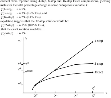
Figure 2 suggests that, the larger is x, the greater is the proportional error in y. This observation leads to the idea of breaking large changes in X into a number of steps, as shown in Figure 3. For each sub-change in X, we use the linear approximation to derive the consequent sub-sub-change in Y. Then, using the new values of X and Y, we recompute the coefficient matrices GY and GX. The process is repeated for each step. If we use 3 steps (see Figure 3), the final value of Y, Y3, is closer to Yexact than was the Johan-sen estimate YJ. We can show, in fact, that given sensible restrictions on the derivatives of F(Y,X), we can obtain a solution as accurate as we like by dividing the process into sufficiently many steps.
4
Y
1 step
Exact
X
X0 X
Y0
Yexact
F YJ
dX dY
Figure 2. Linearisation error
The technique illustrated in Figure 3, known as the Euler method, is the simplest of several related techniques of numerical integration—the process of using differential equations (change formulae) to move from one solution to another. GEMPACK offers the choice of several such techniques. Each re-quires the user to supply an initial solution {Y0,X0}, formulae for the derivative matrices G
Y and GX, and the total percentage change in the exogenous variables, x. The levels functional form, F(Y,X), need not be specified, although it underlies GY and GX.
The accuracy of multistep solution techniques can be improved by extrapolation. Suppose the same experiment were repeated using 4-step, 8-step and 16-step Euler computations, yielding the following estimates for the total percentage change in some endogenous variable Y:
y(4-step) = 4.5%,
y(8-step) = 4.3% (0.2% less), and y(16-step) = 4.2% (0.1% less).
Extrapolation suggests that the 32-step solution would be: y(32-step) = 4.15% (0.05% less),
and that the exact solution would be: y(∞-step) = 4.1%.
Y
1 step
3 step Exact
X
X0 X1 X2 X3
Y0 Y1
Y3 Yexact Y2
XF YJ
The extrapolated result requires 28 (= 4+8+16) steps to compute but would normally be more accurate than that given by a single 28-step computation. Alternatively, extrapolation enables us to obtain given accuracy with fewer steps. As we noted above, each step of a multi-step solution requires: computation from data of the percentage-change derivative matrices GY and GX; solution of the linear system (6); and use of that solution to update the data (X,Y).
In practice, for typical AGE models, it is unnecessary, during a multistep computation, to record values for every element in X and Y. Instead, we can define a set of datacoefficientsV, which are func-tions of X and Y, i.e., V = H(X,Y). Most elements of V are simple cost or expenditure flows such as appear in input-output tables. GY and GX turn out to be simple functions of V; often indeed identical to elements of V. After each small change, V is updated using the formula v = HY(X,Y)y + HX(X,Y)x. The advantages of storing V, rather than X and Y, are twofold:
• the expressions for GY and GX in terms of V tend to be simple, often far simpler than the original F
functions; and
• there are fewer elements in V than in X and Y (e.g., instead of storing prices and quantities sepa-rately, we store merely their products, the values of commodity or factor flows).
3.1. Levels and linearised systems compared: a small example
To illustrate the convenience of the linear approach5, we consider a very small equation system: the CES input demand equations for a producer who makes output Z from N inputs Xk, k=1-N, with prices Pk. In the levels the equations are (see Appendix A):
Xk = Z δ1/(ρ+1)k
[
PPkave
]
−1/(ρ+1), k=1,N (8)
where Pave =
(
∑
i=1 Nδ1/(ρ+1)i Pρ/(ρ+1)i
)
(ρ+1)/ρ. (9)The δk and ρ are behavioural parameters. To solve the model in the levels, the values of the δk are nor-mally found from historical flows data, Vk=PkXk, presumed consistent with the equation system and with some externally given value for ρ. This process is called calibration. To fix the Xk, it is usual to as-sign arbitrary values to the Pk, say 1. This merely sets convenient units for the Xk (base-period-dollars-worth). ρ is normally given by econometric estimates of the elasticity of substitution, σ (=1/(ρ+1)). With the Pk, Xk, Z and ρ known, the δk can be deduced.
In the solution phase of the levels model, δk and ρ are fixed at their calibrated values. The solution algorithm attempts to find Pk, Xk and Z consistent with the levels equations and with other exogenous restrictions. Typically this will involve repeated evaluation of both (8) and (9)—corresponding to
F(Y,X)—and of derivatives which come from these equations—corresponding to FY and FX.
The percentage-change approach is far simpler. Corresponding to (8) and (9), the linearised equa-tions are (see Appendices A and E):
xk = z - σ
(
pk - pave)
, k=1,N (10)and pave =
∑
i=1 NSipi, where the Si are cost shares, eg, Si= Vi
/
∑
k=1 NVk (11)
Since percentage changes have no units, the calibration phase—which amounts to an arbitrary choice of units—is not required. For the same reason the δk parameters do not appear. However, the flows data Vk again form the starting point. After each change they are updated by:
Vk,new =Vk,old + Vk,old(xk + pk)/100 (12) GEMPACK is designed to make the linear solution process as easy as possible. The user specifies the linear equations (10) and (11) and the update formulae (12) in the TABLO language—which re-sembles algebraic notation. Then GEMPACK repeatedly:
5
• evaluates GY and GX at given values of V;
• solves the linear system to find y, taking advantage of the sparsity of GY and GX; and • updates the data coefficients V.
The housekeeping details of multistep and extrapolated solutions are hidden from the user. Apart from its simplicity, the linearised approach has two further advantages.
• It allows free choice of which variables are to be exogenous or endogenous. Many levels algorithms do not allow this flexibility.
• To reduce AGE models to manageable size, it is often necessary to use model equations to substitute out matrix variables of large dimensions. In a linear system, we can always make any variable the subject of any equation in which it appears. Hence, substitution is a simple mechanical process. In fact, because GEMPACK performs this routine algebra for the user, the model can be specified in terms of its original behavioural equations, rather than in a reduced form. This reduces the potential for error and makes model equations easier to check.
3.2. The initial solution
Our discussion of the solution procedure has so far assumed that we possess an initial solution of the model—{Y0,X0} or the equivalent V0—and that results show percentage deviations from this initial state.
In practice, the PHILGEM database does not, like B in Figure 1, show the expected state of the econ-omy at a future date. Instead the most recently available historical data, A, are used. At best, these refer to the present-day economy. Note that, for the atemporal static model, A provides a solution for period T. In the static model, setting all exogenous variables at their base-period levels would leave all the en-dogenous variables at their base-period levels. Nevertheless, A may not be an empirically plausible control state for the economy at period T and the question therefore arises: are estimates of the B-to-C percentage changes much affected by starting from A rather than B? For example, would the percentage effects of a tariff cut inflicted in 1994 differ much from those caused by a 2005 cut? Probably not. First, balanced growth, i.e., a proportional enlargement of the model database, just scales equation coefficients equally; it does not affect PHILGEM results. Second, compositional changes, which do alter percentage-change effects, happen quite slowly. So for short- and medium-run simulations A is a reasonable proxy for B, (Dixon, Parmenter and Rimmer, 1986).6
4. The Equations of PHILGEM
In this section we provide a formal description of the linear form of the model. Our description is organ-ised around the TABLO file which implements the model in GEMPACK.We present the complete text of the TABLO Input file divided into a sequence of excerpts and supplemented by tables, figures and ex-planatory text.
The TABLO language in which the file is written is essentially conventional algebra, with names for variables and coefficients chosen to be suggestive of their economic interpretations. Some practice is required for readers to become familiar with the TABLO notation but it is no more complex than alterna-tive means of setting out the model—the notation employed in DPSV (1982), for example. Acquiring the familiarity allows ready access to the GEMPACK programs used to conduct simulations with the model and to convert the results to human-readable form. Both the input and the output of these programs em-ploy the TABLO notation. Moreover, familiarity with the TABLO format is essential for users who may wish to make modifications to the model's structure.
6
Another compelling reason for using the TABLO Input file to document the model is that it ensures that our description is complete and accurate: complete because the only other data needed by the GEMPACK solution process is numerical (the model's database and the exogenous inputs to particular simulations); and accurate because GEMPACK is nothing more than an equation solving system, incor-porating no economic assumptions of its own.
We continue this section with a short introduction to the TABLO language—other details may be picked up later, as they are encountered. Then we describe the input-output database which underlies the model. This structures our subsequent presentation.
4.1. The TABLO language
The TABLO model description defines the percentage-change equations of the model. For example, the CES demand equations, (10) and (11), would appear as:
Equation E_x # input demands #
(all, f, FAC) x(f) = z ‐ SIGMA*[p(f) ‐ p_f]; Equation E_p_f # input cost index #
V_F*p_f = sum{f,FAC, V(f)*p(f)};
The first word, 'Equation', is a keyword which defines the statement type. Then follows the identifier for the equation, which must be unique. The descriptive text between '#' symbols is optional—it appears in certain report files. The expression '(all, f, FAC)' signifies that the equation is a matrix equation, contain-ing one scalar equation for each element of the set FAC.7
Within the equation, the convention is followed of using lower-case letters for the percentage-change variables (x, z, p and p_f), and upper case for the coefficients (SIGMA, V and V_F). Since GEMPACK ignores case, this practice assists only the human reader. An implication is that we cannot use the same sequence of characters, distinguished only by case, to define a variable and a coefficient. The '(f)' suffix indicates that variables and coefficients are vectors, with elements corresponding to the set FAC. A semi-colon signals the end of the TABLO statement.
To facilitate portability between computing environments, the TABLO character set is quite re-stricted—only alphanumerics and a few punctuation marks may be used. The use of Greek letters and subscripts is precluded, and the asterisk, '*', must replace the multiplication symbol '×'.
Sets, coefficients and variables must be explicitly declared, via statements such as:
Set FAC # inputs # (capital, labour, energy); Coefficient
(all,f,FAC) V(f) # cost of inputs #; V_F # total cost #;
SIGMA # substitution elasticity #; Variable
(all,f,FAC) p(f) # price of inputs #; (all,f,FAC) x(f) # demand for inputs #; z # output #;
p_f # input cost index #;
As the last two statements in the 'Coefficient' block and the last three in the 'Variable' block illustrate, initial keywords (such as 'Coefficient' and 'Variable') may be omitted if the previous statement was of the same type.
Coefficients must be assigned values, either by reading from file:
Read V from file FLOWDATA; Read SIGMA from file PARAMS;
or in terms of other coefficients, using formulae:
Formula V_F = sum{f, FAC, V(f)}; ! used in cost index equation !
7
The right hand side of the last statement employs the TABLO summation notation, equivalent to the
Σ
notation used in standard algebra. It defines the sum over an index f running over the set FAC of the in-put-cost coefficients, V(f). The statement also contains a comment, i.e., the text between exclamation marks (!). TABLO ignores comments.Some of the coefficients will be updated during multistep computations. This requires the inclusion of statements such as:
Update (all,f,FAC) V(f) = x(f)*p(f);
which is the default update statement, causing V(f) to be increased after each step by [x(f) + p(f)]%, where x(f) and p(f) are the percentage changes computed at the previous step.
The sample statements listed above introduce most of the types of statement required for the model. But since all sets, variables and coefficients must be defined before they are used, and since coefficients must be assigned values before appearing in equations, it is necessary for the order of the TABLO state-ments to be almost the reverse of the order in which they appear above. The PHILGEM TABLO Input file is ordered as follows:
•
definition of sets;•
declarations of variables;•
declarations of often-used coefficients which are read from files, with associated Read and Update statements;•
declarations of other often-used coefficients which are computed from the data, using associated Formulae; and•
groups of topically-related equations, with some of the groups including statements defining coeffi-cients which are used only within that group.4.2. The naming system
PHILGEM’s naming convention is the same as ORANI-G. The TABLO Input file defines a multitude of variables and coefficients that are used in the model's equations. It can be difficult to remember the names of all these variables and coefficients8. Fortunately, their names follow a pattern. Although GEMPACK does not require that names conform to any pattern, we find that systematic naming reduces the burden on (human) memory. As far as possible, names for variables and coefficients conform to a system in which each name consists of 2 or more parts, as follows:
first, a letter or letters indicating the type of variable, for example, a technical change
del ordinary (rather than percentage) change f shift variable
H indexing parameter p price, local currency pf price, foreign currency S input share
SIGMA elasticity of substitution
t tax
V levels value, local currency
w percentage-change value, local currency x input quantity;
second, one of the digits 0 to 6 indicating user, that is, 1 current production
2 investment 3 consumption
8
4 export 5 government 6 inventories
0 all users, or user distinction irrelevant;
third (optional), three or more letters giving further information, for example, bas (often omitted) basic—not including margins or taxes
cap capital
cif imports at border prices imp imports (duty paid)
lab labour
lnd land
lux linear expenditure system (supernumerary part)
mar margins
oct other cost tickets
prim all primary factors (land, labour or capital) pur at purchasers' prices
sub linear expenditure system (subsistence part)
tar tariffs
tax indirect taxes
tot total or average over all inputs for some user
hou households
gov government
ent enterprises
row rest of the world gos gross operating surplus;
fourth (optional), an underscore character, indicating that this variable is an aggregate or average, with subsequent letters showing over which sets the underlying variable has been summed or averaged, for example,
_c over COM (commodities), _s over SRC (dom + imp), _i over IND (industries), _io over IND and OCC (skills).
Although GEMPACK does not distinguish between upper and lower case, we use: lower case for variable names and set indices;
upper case for set and coefficient names; and initial letter upper case for TABLO keywords.
4.3. The model's data base
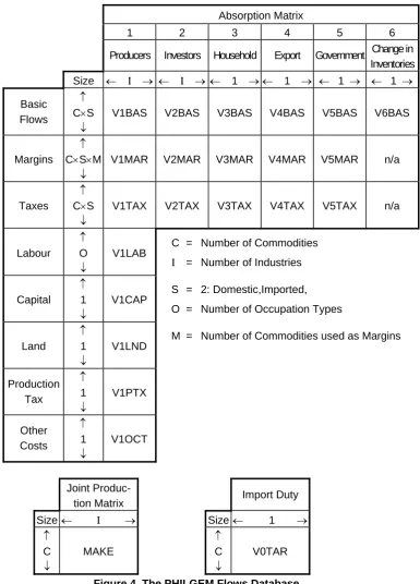
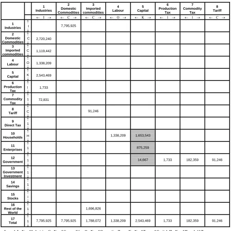
Figure 4 is a schematic representation of PHILGEM's input-output table database. It reveals the basic structure of the model. The column headings in the main part of the figure (an absorption matrix or Supply-Use Table) identify the following demanders:
(1) domestic producers divided into I industries; (2) investors divided into I industries;
(3) a single representative household;
(4) an aggregate foreign purchaser of exports; (5) government demands; and
(6) changes in inventories.
to or subtracted from inventories. Only domestically produced goods appear in the export column. M of the domestically produced goods are used as margins services (wholesale and retail trade, and transport) which are required to transfer commodities from their sources to their users. Commodity taxes are payable on the purchases. As well as intermediate inputs, current production requires inputs of three categories of primary factors: labour (divided into O occupations), fixed capital, and agricultural land. Production taxes include output taxes or subsidies that are not user-specific. The 'other costs' category covers various miscellaneous taxes on firms, such as municipal taxes or charges.
Absorption Matrix
1 2 3 4 5 6
Producers Investors Household Export Government Change in Inventories
Size ← I → ← I → ← 1 → ← 1 → ← 1 → ← 1 →
Basic Flows
↑ C×S
↓
V1BAS V2BAS V3BAS V4BAS V5BAS V6BAS
Margins ↑ C×S×M
↓
V1MAR V2MAR V3MAR V4MAR V5MAR n/a
Taxes
↑ C×S
↓
V1TAX V2TAX V3TAX V4TAX V5TAX n/a
Labour ↑ O ↓
V1LAB C = Number of Commodities
I = Number of Industries
Capital ↑ 1 ↓
V1CAP
S = 2: Domestic,Imported, O = Number of Occupation Types
Land
↑ 1 ↓
V1LND
M = Number of Commodities used as Margins
Production Tax
↑ 1 ↓
V1PTX
Other Costs
↑ 1 ↓
V1OCT
Joint
Produc-tion Matrix Import Duty Size ← I → Size← 1 →
↑ C ↓
MAKE
↑ C ↓
V0TAR
Each cell in the illustrative absorption matrix in Figure 4 contains the name of the corresponding data matrix. For example, V2MAR is a 4-dimensional array showing the cost of M margins services on the flows of C goods, both domestically produced and imported (S), to I investors.
In principle, each industry is capable of producing any of the C commodity types. The MAKE matrix at the bottom of Figure 4 shows the value of output of each commodity by each industry. Finally, tariffs on imports are assumed to be levied at rates which vary by commodity but not by user. The revenue obtained is represented by the tariff vector V0TAR.
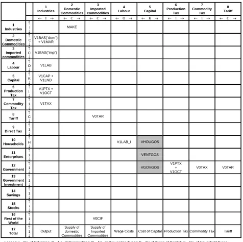
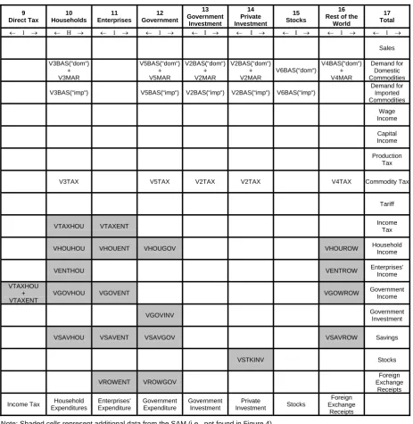
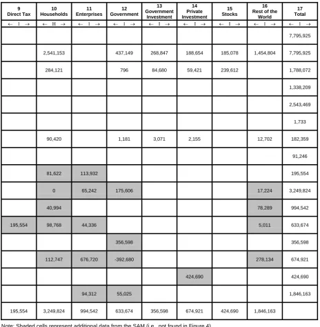
Figure 5 presents a schematic representation of the entire database of PHILGEM in the form of a Social Accounting Matrix (SAM), while Figure 6 presents the value flows of the SAM which is based on the Input-Output Table and National Accounts data (NSCB 2006), both for the year 2000.
A SAM is an integrated framework that records all transactions in an economy in a given year (Round, 2003). It provides information on the economic and social structure; illuminates the interaction of various agents; and captures economic flows at both micro and macro levels.
A SAM tracks how income is generated and distributed. It is a square matrix, composed of different accounts, with entries along the rows representing receipts while column entries track expenditures. A SAM adheres to double entry accounting in which a flow is both recorded as a receipt and an expense. A residual savings row allows the row sum for each account to equal the corresponding column sum. The Philippine SAM shown in Figure 5 is based on a combination of data coming from the input-output table, national income and product accounts, household survey and the labour force survey.
Figure 5 reveals that the first 8 rows of the SAM correspond to the Input-Output table database shown in Figure 4, while entries found along the intersection of government row and column accounts representing commodity tax, production tax and tariff are computed directly. On the other hand, cells shaded in gray represent data drawn elsewhere or not found in the input-output table.
Entries in the SAM are named based on the row and column in which they appear. For example, VHOUGOS represents the value of household income from gross operating surplus (or capital), while VTAXENT corresponds to the value of direct income taxes paid by enterprises. VGOVROW shows the value of foreign aid received by the government whereas VGOVENT displays the value of dividend income received by government from enterprises which include both public and private corporations. Section 5 contains more details of the SAM and associated equations and variables.
The capital income shares of these agents are sourced from the national income accounts for the year 2000 (NSCB 2006). In turn, each household’s share in total capital income earned by all households in the economy is taken from the 2003 household survey, known locally as the family income and expenditure survey (NSO 2003).
1 Industries 2 Domestic Commodities 3 Imported commodities 4 Labour 5 Capital 6 Production Tax 7 Commodity Tax 8 Tariff
← I → ← C → ← C → ← O → ← K → ← 1 → ← 1 → ← C →
1 Industries ↑ I ↓ MAKE 2 Domestic Commodities ↑ C ↓ V1BAS(“dom“) + V1MAR 3 Imported commodities ↑ C ↓ V1BAS(“imp“) 4 Labour ↑ O ↓ V1LAB 5 Capital ↑ K ↓ V1CAP + V1LND 6 Production Tax ↑ 1 ↓ V1PTX + V1OCT 7 Commodity Tax ↑ 1 ↓ V1TAX 8 Tariff ↑ C ↓ V0TAR 9 Direct Tax ↑ 1 ↓ 10 Households ↑ H ↓ V1LAB_I VHOUGOS 11 Enterprises ↑ 1 ↓ VENTGOS 12 Government ↑ 1 ↓ VGOVGOS V1PTX + V1OCT V0TAX V0TAR 13 Government Investment ↑ 1 ↓ 14 Savings ↑ 1 ↓ 15 Stocks ↑ i ↓ 16 Rest of the
World ↑ 1 ↓ V0CIF 17 Total ↑ 1 ↓ Output Supply of domestic Commodities Supply of Imported Commodities
Wage Costs Cost of Capital Production Tax Commodity Tax Tariff Legend: I – No. of Industries; C – No. of Commodities; O – No. of Occupation Types; K – No.of Types of Capital; H – No. of Household Types.
9 Direct Tax 10 Households 11 Enterprises 12 Government 13 Government Investment 14 Private Investment 15 Stocks 16 Rest of the
World
17 Total
← 1 → ← H → ← 1 → ← 1 → ← I → ← I → ← I → ← 1 → ← 1 →
Sales V3BAS(“dom“) + V3MAR V5BAS(“dom“) + V5MAR V2BAS(“dom“) + V2MAR V2BAS(“dom“) + V2MAR V6BAS(“dom“) V4BAS(“dom“) + V4MAR Demand for Domestic Commodities V3BAS(“imp“) V5BAS(“imp“) V2BAS(“imp“) V2BAS(“imp“) V6BAS(“imp“)
Demand for Imported Commodities Wage Income Capital Income Production Tax V3TAX V5TAX V2TAX V2TAX V4TAX Commodity Tax
Tariff
VTAXHOU VTAXENT Income
Tax VHOUHOU VHOUENT VHOUGOV VHOUROW Household
Income
VENTHOU VENTROW Enterprises’
Income VTAXHOU
+ VTAXENT
VGOVHOU VGOVENT VGOWROW Government
Income
VGOVINV Government
Investment VSAVHOU VSAVENT VSAVGOV VSAVROW Savings
VSTKINV Stocks
VROWENT VROWGOV
Foreign Exchange
Receipts Income Tax Household
Expenditures Enterprises’ Expenditure Government Expenditure Government Investment Private Investment Stocks Foreign Exchange Receipts
Note: Shaded cells represent additional data from the SAM (i.e., not found in Figure 4).
1 Industries 2 Domestic Commodities 3 Imported commodities 4 Labour 5 Capital 6 Production Tax 7 Commodity Tax 8 Tariff
← I → ← C → ← C → ← O → ← K → ← 1 → ← 1 → ← C →
1 Industries ↑ I ↓ 7,795,925 2 Domestic Commodities ↑ C ↓ 2,720,240 3 Imported commodities ↑ C ↓ 1,119,442 4 Labour ↑ O ↓ 1,338,209 5 Capital ↑ K ↓ 2,543,469 6 Production Tax ↑ 1 ↓ 1,733 7 Commodity Tax ↑ 1 ↓ 72,831 8 Tariff ↑ C ↓ 91,246 9 Direct Tax ↑ 1 ↓ 10 Households ↑ H ↓ 1,338,209 1,653,543 11 Enterprises ↑ 1 ↓ 875,259 12 Government ↑ 1 ↓
14,667 1,733 182,359 91,246
13 Government Investment ↑ 1 ↓ 14 Savings ↑ 1 ↓ 15 Stocks ↑ i ↓ 16 Rest of the
World ↑ 1 ↓ 1,696,826 17 Total ↑ 1 ↓
7,795,925 7,795,925 1,788,072 1,338,209 2,543,469 1,733 182,359 91,246
Legend: I – No. of Industries; C – No. of Commodities; O – No. of Occupation Types; K – No.of Types of Capital; H – No. of Household Types.
9 Direct Tax
10 Households
11 Enterprises
12 Government
13 Government
Investment
14 Private Investment
15 Stocks
16 Rest of the
World
17 Total
← 1 → ← H → ← 1 → ← 1 → ← I → ← I → ← I → ← 1 → ← 1 →
7,795,925
2,541,153 437,149 268,847 188,654 185,078 1,454,804 7,795,925
284,121 796 84,680 59,421 239,612 1,788,072
1,338,209
2,543,469
1,733
90,420 1,181 3,071 2,155 12,702 182,359
91,246
81,622 113,932 195,554
0 65,242 175,606 17,224 3,249,824
40,994 78,289 994,542
195,554 98,768 44,336 5,011 633,674
356,598 356,598
112,747 676,720 -392,680 278,134 674,921
424,690 424,690
94,312 55,025 1,846,163
195,554 3,249,824 994,542 633,674 356,598 674,921 424,690 1,846,163
Note: Shaded cells represent additional data from the SAM (i.e., not found in Figure 4).
Figure 6. (continued). PHILGEM Aggregate Social Accounting Matrix (SAM) Database
4.4. Dimensions of the model
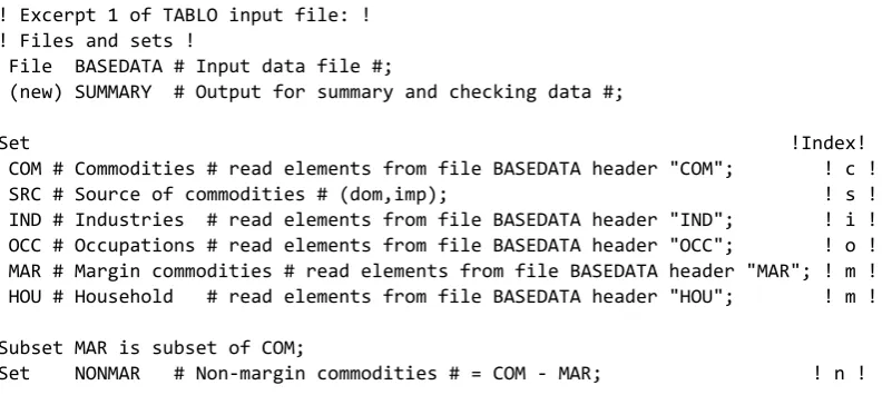
Excerpt 1 of the TABLO Input file begins by defining logical names for input and output files. Initial data are stored in the BASEDATA input file. The SUMMARY output file is used to store summary and diagnostic information. Note that BASEDATA and SUMMARY are logical names. The actual locations of these files (disk, folder, filename) are chosen by the model user.
! Excerpt 1 of TABLO input file: ! ! Files and sets !
File BASEDATA # Input data file #;
(new) SUMMARY # Output for summary and checking data #;
Set !Index! COM # Commodities # read elements from file BASEDATA header "COM"; ! c ! SRC # Source of commodities # (dom,imp); ! s ! IND # Industries # read elements from file BASEDATA header "IND"; ! i ! OCC # Occupations # read elements from file BASEDATA header "OCC"; ! o ! MAR # Margin commodities # read elements from file BASEDATA header "MAR"; ! m ! HOU # Household # read elements from file BASEDATA header "HOU"; ! m !
Subset MAR is subset of COM;
Set NONMAR # Non‐margin commodities # = COM ‐ MAR; ! n !
The commodity, industry, occupational, and household classifications of PHILGEM described here are aggregates of the classifications used in the original version of PHILGEM, which had 240 industries and commodities, 10 labour occupations, and 42,092 households.
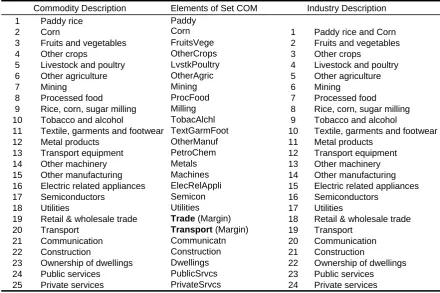
The industry classification differs slightly from the commodity classification. Both are listed in Table 1. In this aggregated version of the model, multiproduction is confined to the first industry (RiceCorn), which produce the first two commodities (Paddy rice and Corn). Each of the remaining industries produces a unique commodity. Labour is disaggregated into skill-based occupational categories described by the set OCC.
The central column of Table 1 lists the elements of the set COM which are read from file. GEMPACK uses the element names to label the rows and columns of results and data tables. The ele-ment names cannot be more than 12 letters long, nor contain spaces. The IND eleele-ments are the same as elements 2-25 of COM. The representative households are lThe set HOU contains elements sh the representative households by demographic charac are also read from file
Elements of the set MAR are margins commodities, i.e., they are required to facilitate the flows of other commodities from producers (or importers) to users. Hence, the costs of margins services, together with indirect taxes, account for differences between basic prices (received by producers or importers) and purchasers' prices (paid by users).
TABLO does not prevent elements of two sets from sharing the same name; nor, in such a case, does it automatically infer any connection between the corresponding elements. The Subset statement which follows the definition of the set MAR is required for TABLO to realize that the two elements of MAR, Trade and Transport, are the same as the 19th and 20th elements of the set COM.
Table 1 Commodity and Industry Classification
Commodity Description Elements of Set COM Industry Description Paddy
Corn Paddy rice and Corn 1
2 3
Paddy rice Corn
Fruits and vegetables FruitsVege
1
2 Fruits and vegetables 4 Other crops OtherCrops 3 Other crops
5 Livestock and poultry LvstkPoultry 4 Livestock and poultry 6 Other agriculture OtherAgric 5 Other agriculture
7 Mining Mining 6 Mining
8 Processed food ProcFood 7 Processed food 9 Rice, corn, sugar milling Milling 8 Rice, corn, sugar milling 10 Tobacco and alcohol TobacAlchl 9 Tobacco and alcohol
11 Textile, garments and footwear TextGarmFoot 10 Textile, garments and footwear 12 Metal products OtherManuf 11 Metal products
13 Transport equipment PetroChem 12 Transport equipment 14 Other machinery Metals 13 Other machinery 15 Other manufacturing Machines 14 Other manufacturing 16 Electric related appliances ElecRelAppli 15 Electric related appliances 17 Semiconductors Semicon 16 Semiconductors
18 Utilities Utilities 17 Utilities
19 Retail & wholesale trade Trade (Margin) 18 Retail & wholesale trade 20 Transport Transport (Margin) 19 Transport
21 Communication Communicatn 20 Communication 22 Construction Construction 21 Construction
23 Ownership of dwellings Dwellings 22 Ownership of dwellings 24 Public services PublicSrvcs 23 Public services 25 Private services PrivateSrvcs 24 Private services
The next statement relates to the household set. Initially, the elements of the set GENDER (female and male) are listed explicitly while the set DEC is specified to contain 10 ordered elements representing income deciles 1 to 10. On the other hand, a new set HOU is generated as a set (Cartesian) product of the sets GENDER and DEC, resulting in HOU containing all possible ordered pairs coming from the sets GENDER and DEC respectively. Accordingly, set HOU would now contain elements: female_dec01, male_dec01, female_dec02, male_dec02,...,female_dec10, male_dec10. Note that under this operation, the elements of the set GENDER vary faster while those of the set DEC vary slower; and a joining charater "_" that distinguishes the elements of the first and second set is automatically created (see section 9.1.4 of GEMPACK user manual for more details).
4.5. Core data coefficients and related variables
The next excerpts of the TABLO file contains statements indicating coefficient names data to be read from file. The data items defined in these statements appear as coefficients in the model's equations. The statements define coefficient names (which all appear in upper-case characters), the locations from which the data are to be read, variable names (in lower-case), and formulae for the data updates which are necessary in computing multi-step solutions to the model (see Section 3).
4.5.1. Basic flows
The excerpts group the data according to the rows of Figure. Thus, Excerpt 2 begins by defining coef-ficients representing the basic commodity flows corresponding to row 1 (direct flows) of the figure, i.e., the flow matrices V1BAS, V2BAS, and so on. Preceding the coefficient names are their dimensions, indicated using the "all" qualifier and the sets defined in Excerpt 1. For example, the first 'Coefficient' statement defines a data item V1BAS(c,s,i) which is the basic value (indicated by 'BAS') of a flow of intermediate inputs (indicated by '1') of commodity c from source s to user industry i. The first 'Read' statement indicates that this data item is stored on file BASEDATA with header '1BAS'. (A GEMPACK data file consists of a number of data items such as arrays of real numbers. Each data item is identified by a unique key or 'header').
appear in lower-case letters. Preceding the names of the variables are their dimensions, indicated using the sets defined in Excerpt 1. For example, the first variable statement defines a matrix variable x1 (in-dexed by commodity, source, and using industry) the elements of which are percentage changes in the direct demands by producers for source-specific intermediate inputs. This is the quantity variable corre-sponding to V1BAS.
The last in the group of quantity variables, delx6, is preceded by the 'Change' qualifier to indicate that it is an ordinary (rather than percentage) change. Changes in inventories may be either positive or negative. Our multistep solution procedure requires that large changes be broken into a sequence of small changes. However, no sequence of small percentage changes allows a number to change sign—at least one change must exceed -100%. Thus, for variables that may, in the levels, change sign, we prefer to use ordinary changes. The names of ordinary change variables often start with the letters "del".
Next come two price variables. A matrix variable p0 (indexed by commodity and source), shows percentage changes in the basic prices which are common to all local users. These basic prices do not include the cost of margins and taxes. Exports have their own basic prices, pe. Potentially, the pe could be different from the domestic part of p09.
! Excerpt 2 of TABLO input file: !
! Data coefficients and variables relating to basic commodity flows ! Coefficient ! Basic flows of commodities (excluding margin demands)!
(all,c,COM)(all,s,SRC)(all,i,IND) V1BAS(c,s,i) # Intermediate basic flows #; (all,c,COM)(all,s,SRC)(all,i,IND) V2BAS(c,s,i) # Investment basic flows #; (all,c,COM)(all,s,SRC) V3BAS(c,s) # Household basic flows #; (all,c,COM) V4BAS(c) # Export basic flows #; (all,c,COM)(all,s,SRC) V5BAS(c,s) # Government basic flows #; (all,c,COM)(all,s,SRC) V6BAS(c,s) # Inventories basic flows #;
Read
V1BAS from file BASEDATA header "1BAS"; V2BAS from file BASEDATA header "2BAS"; V3BAS from file BASEDATA header "3BAS"; V4BAS from file BASEDATA header "4BAS"; V5BAS from file BASEDATA header "5BAS"; V6BAS from file BASEDATA header "6BAS";
Variable ! Variables used to update above flows !
(all,c,COM)(all,s,SRC)(all,i,IND) x1(c,s,i) # Intermediate basic demands #; (all,c,COM)(all,s,SRC)(all,i,IND) x2(c,s,i) # Investment basic demands #; (all,c,COM)(all,s,SRC) x3(c,s) # Household basic demands #; (all,c,COM) x4(c) # Export basic demands #; (all,c,COM)(all,s,SRC) x5(c,s) # Government basic demands #; (change)(all,c,COM)(all,s,SRC) delx6(c,s) # Inventories demands #;
(all,c,COM)(all,s,SRC) p0(c,s) # Basic prices for local users #; (all,c,COM) pe(c) # Basic price of exportables #; (change)(all,c,COM)(all,s,SRC) delV6(c,s) # Value of inventories #;
Update
(all,c,COM)(all,s,SRC)(all,i,IND) V1BAS(c,s,i) = p0(c,s)*x1(c,s,i); (all,c,COM)(all,s,SRC)(all,i,IND) V2BAS(c,s,i) = p0(c,s)*x2(c,s,i); (all,c,COM)(all,s,SRC) V3BAS(c,s) = p0(c,s)*x3(c,s); (all,c,COM) V4BAS(c) = pe(c)*x4(c); (all,c,COM)(all,s,SRC) V5BAS(c,s) = p0(c,s)*x5(c,s); (change)(all,c,COM)(all,s,SRC) V6BAS(c,s) = delV6(c,s);
Finally, the variable delV6 is used in the update statements which appear next.
9
The first 'Update' statement indicates that the flow V1BAS(c,s,i) should be updated using the default update formula, which is used for a data item which is a product of two (or more) of the model's vari-ables. For an item of the form V = PX, the formula for the updated value VUis:
VU = V0 + Δ(PX) = V0 + X0ΔP + P0ΔX
= V0 + P0X0
(
ΔP P0 +ΔX
X0
)
= V0 + V0(
p 100 +x
100
)
(13)where V0, P0 and X0 are the pre-update values, and p and x are the percentage changes of the variables P and X. For the data item V1BAS(c,s,i) the relevant percentage-change variables are p0(c,s) (the basic-value price of commodity c from source s) and x1(c,s,i) (the demand by user industry i for intermediate inputs of commodity c from source s).
Not all of the model's data items are amenable to update via default Updates. For example, the in-ventories flows, V6BAS, might change sign, and so must not be updated with percentage change variables. In such a case, the Update statement must contain an explicit formula for the ordinary change in the data item: this is indicated by the word 'Change' in parentheses. For V6BAS we represent the change by an ordinary-change variable, delV6. The Update formula (13) then becomes simply:
VU = V0 + ΔV. (14)
An equation defining the delV6 variable appears later on.
4.5.2. Margin flows
The coefficients and variables of Excerpt 3 are associated with row 2 (margins) of Figure 4, i.e., the flow matrices V1MAR, V2MAR, and so on. These are the quantities of retail and wholesale services or transport needed to deliver each basic flow to the user. For example V3MAR(c,s,m) is the value of mar-gin type m used to deliver commodity type c from source s to households (user 3). The model assumes that margin services are domestically produced and are valued at basic prices—represented by the variable p0dom, which (we shall see later) is simply a synonym for the domestic part of the basic price matrix, p0 [i.e., p0dom(c) = p0(c,"dom")].
! Excerpt 3 of TABLO input file: !
! Data coefficients and variables relating to margin flows ! Coefficient
(all,c,COM)(all,s,SRC)(all,i,IND)(all,m,MAR)
V1MAR(c,s,i,m) # Intermediate margins #; (all,c,COM)(all,s,SRC)(all,i,IND)(all,m,MAR)
V2MAR(c,s,i,m) # Investment margins #; (all,c,COM)(all,s,SRC)(all,m,MAR) V3MAR(c,s,m) # Households margins #; (all,c,COM)(all,m,MAR) V4MAR(c,m) # Export margins #; (all,c,COM)(all,s,SRC)(all,m,MAR) V5MAR(c,s,m) # Government margins #; Read
V1MAR from file BASEDATA header "1MAR"; V2MAR from file BASEDATA header "2MAR"; V3MAR from file BASEDATA header "3MAR"; V4MAR from file BASEDATA header "4MAR"; V5MAR from file BASEDATA header "5MAR";
Variable ! Variables used to update above flows ! (all,c,COM)(all,s,SRC)(all,i,IND)(all,m,MAR)
x1mar(c,s,i,m)# Intermediate margin demand #; (all,c,COM)(all,s,SRC)(all,i,IND)(all,m,MAR)
x2mar(c,s,i,m)# Investment margin demands #; (all,c,COM)(all,s,SRC)(all,m,MAR) x3mar(c,s,m) # Household margin demands #; (all,c,COM)(all,m,MAR) x4mar(c,m) # Export margin demands #; (all,c,COM)(all,s,SRC)(all,m,MAR) x5mar(c,s,m) # Government margin demands #; (all,c,COM) p0dom(c) # Basic price of domestic goods = p0(c,"dom") #;
Update
(all,c,COM)(all,s,SRC)(all,i,IND)(all,m,MAR)
V2MAR(c,s,i,m) = p0dom(m)*x2mar(c,s,i,m); (all,c,COM)(all,s,SRC)(all,m,MAR) V3MAR(c,s,m) = p0dom(m)*x3mar(c,s,m); (all,c,COM)(all,m,MAR) V4MAR(c,m) = p0dom(m)*x4mar(c,m); (all,c,COM)(all,s,SRC)(all,m,MAR) V5MAR(c,s,m) = p0dom(m)*x5mar(c,s,m);
4.5.3. User-specific commodity taxes
Excerpt 4 contains coefficients and variables associated with row 3 (commodity taxes) of Figure 4, i.e., the flow matrices V1TAX, V2TAX, and so on. These all have the same dimensions as the corre-sponding basic flows.
! Excerpt 4 of TABLO input file: !
! Data coefficients and variables relating to commodity taxes ! Coefficient ! Taxes on Basic Flows!
(all,c,COM)(all,s,SRC)(all,i,IND) V1TAX(c,s,i) # Taxes on intermediate #; (all,c,COM)(all,s,SRC)(all,i,IND) V2TAX(c,s,i) # Taxes on investment #; (all,c,COM)(all,s,SRC) V3TAX(c,s) # Taxes on households #; (all,c,COM) V4TAX(c) # Taxes on export #; (all,c,COM)(all,s,SRC) V5TAX(c,s) # Taxes on government #; Read
V1TAX from file BASEDATA header "1TAX"; V2TAX from file BASEDATA header "2TAX"; V3TAX from file BASEDATA header "3TAX"; V4TAX from file BASEDATA header "4TAX"; V5TAX from file BASEDATA header "5TAX"; Variable
(change)(all,c,COM)(all,s,SRC)(all,i,IND) delV1TAX(c,s,i) # Interm tax rev #; (change)(all,c,COM)(all,s,SRC)(all,i,IND) delV2TAX(c,s,i) # Invest tax rev #; (change)(all,c,COM)(all,s,SRC) delV3TAX(c,s) # H'hold tax rev #; (change)(all,c,COM) delV4TAX(c) # Export tax rev #; (change)(all,c,COM)(all,s,SRC) delV5TAX(c,s) # Govmnt tax rev #; Update
(change)(all,c,COM)(all,s,SRC)(all,i,IND) V1TAX(c,s,i) = delV1TAX(c,s,i); (change)(all,c,COM)(all,s,SRC)(all,i,IND) V2TAX(c,s,i) = delV2TAX(c,s,i); (change)(all,c,COM)(all,s,SRC) V3TAX(c,s) = delV3TAX(c,s); (change)(all,c,COM) V4TAX(c) = delV4TAX(c); (change)(all,c,COM)(all,s,SRC) V5TAX(c,s) = delV5TAX(c,s);
PHILGEM treats commodity taxes in great detail—the tax levied on each basic flow is separately identi-fied. Published input-output tables are usually less detailed—so to construct the initial model database we enforce plausible assumptions: e.g., that all intermediate usage of, say, Coal, is taxed at the same rate. However, the disaggregated data structure still allows us to simulate the effects of commodity-and-user-specific tax changes, such as an increased tax on Coal used by the Iron industry.
The tax flows are updated by corresponding ordinary change variables: equations determining these appear later on.
4.5.4. Factor payments and other flows data
Excerpt 5 of the TABLO Input file corresponds to the remaining rows of Figure 4. There are coefficient matrices for payments to labour, capital, and land, and 2 sorts of production tax. Then are listed the cor-responding price and quantity variables. For the production tax V1PTX, the corcor-responding ordinary change variable delV1PTX is used in a Change Update statement: an equation determining this variable appears later. The other flow coefficients in this group are simply the products of prices and quantities. Hence, they can be updated via default Update statements.
Excerpt 5 also defines the import duty vector V0TAR. Treatment of the last item in the flows data-base, the multiproduction matrix MAKE, showing output of commodities by each industry, is deferred to a later section.
! Excerpt 5 of TABLO input file: !
(all,i,IND)(all,o,OCC) V1LAB(i,o) # Wage bill matrix #; (all,i,IND) V1CAP(i) # Capital rentals #; (all,i,IND) V1LND(i) # Land rentals #; (all,i,IND) V1PTX(i) # Production tax #; (all,i,IND) V1OCT(i) # Other cost tickets #; Read
V1LAB from file BASEDATA header "1LAB"; V1CAP from file BASEDATA header "1CAP"; V1LND from file BASEDATA header "1LND"; V1PTX from file BASEDATA header "1PTX"; V1OCT from file BASEDATA header "1OCT"; Variable
(all,i,IND)(all,o,OCC) x1lab(i,o) # Employment by industry and occupation #; (all,i,IND)(all,o,OCC) p1lab(i,o) # Wages by industry and occupation #; (all,i,IND) x1cap(i) # Current capital stock #;
(all,i,IND) p1cap(i) # Rental price of capital #; (all,i,IND) x1lnd(i) # Use of land #;
(all,i,IND) p1lnd(i) # Rental price of land #;
(change)(all,i,IND) delV1PTX(i) # Ordinary change in production tax revenue #; (all,i,IND) x1oct(i) # Demand for "other cost" tickets #;
(all,i,IND) p1oct(i) # Price of "other cost" tickets #; Update
(all,i,IND)(all,o,OCC) V1LAB(i,o) = p1lab(i,o)*x1lab(i,o); (all,i,IND) V1CAP(i) = p1cap(i)*x1cap(i); (all,i,IND) V1LND(i) = p1lnd(i)*x1lnd(i); (change)(all,i,IND) V1PTX(i) = delV1PTX(i); (all,i,IND) V1OCT(i) = p1oct(i)*x1oct(i);
! Data coefficients relating to import duties ! Coefficient (all,c,COM) V0TAR(c) # Tariff revenue #; Read V0TAR from file BASEDATA header "0TAR";
Variable (all,c,COM) (change) delV0TAR(c) # Ordinary change in tariff revenue #; Update (change) (all,c,COM) V0TAR(c) = delV0TAR(c);
4.5.5. Purchasers' values
Excerpt 6 defines the values at purchasers' prices of the commodity flows identified in Figure 4. These aggregates will be used in several different equation blocks. The definitions use the TABLO summation notation, explained in Section 4.1. For example, the first formula in Excerpt 6 contains the term:
sum{m,MAR, V1MAR(c,s,i,m) }
This defines the sum, over an index m running over the set of margins commodities (MAR), of the input-output data flows V1MAR(c,s,i,m). This sum is the total value of margins commodities required to facilitate the flow of intermediate inputs of commodity c from source s to user industry i. Adding this sum to the basic value of the intermediate-input flow and the associated indirect tax, gives the pur-chaser's-price value of the flow.
Next are defined purchasers' price variables, which include basic, margin and tax components. Equations to determine these variables appear in Excerpt 22 below.
! Excerpt 6 of TABLO input file: !
! Coefficients and variables for purchaser's prices (basic + margins + taxes) ! Coefficient ! Flows at purchasers prices !
(all,c,COM)(all,s,SRC)(all,i,IND) V1PUR(c,s,i) # Intermediate purch. value #; (all,c,COM)(all,s,SRC)(all,i,IND) V2PUR(c,s,i) # Investment purch. value #; (all,c,COM)(all,s,SRC) V3PUR(c,s) # Households purch. value #; (all,c,COM) V4PUR(c) # Export purch. value #; (all,c,COM)(all,s,SRC) V5PUR(c,s) # Government purch. value #; Formula
(all,c,COM)(all,s,SRC)(all,i,IND)
V1PUR(c,s,i) = V1BAS(c,s,i) + V1TAX(c,s,i) + sum{m,MAR, V1MAR(c,s,i,m)}; (all,c,COM)(all,s,SRC)(all,i,IND)
V3PUR(c,s) = V3BAS(c,s) + V3TAX(c,s) + sum{m,MAR, V3MAR(c,s,m)}; (all,c,COM)
V4PUR(c) = V4BAS(c) + V4TAX(c) + sum{m,MAR, V4MAR(c,m)}; (all,c,COM)(all,s,SRC)
V5PUR(c,s) = V5BAS(c,s) + V5TAX(c,s) + sum{m,MAR, V5MAR(c,s,m)};
Variable ! Purchasers prices !
(all,c,COM)(all,s,SRC)(all,i,IND) p1(c,s,i)# Purchaser's price, intermediate #; (all,c,COM)(all,s,SRC)(all,i,IND) p2(c,s,i)# Purchaser's price, investment #; (all,c,COM)(all,s,SRC) p3(c,s) # Purchaser's price, household #; (all,c,COM) p4(c) # Purchaser's price, exports,loc$ #; (all,c,COM)(all,s,SRC) p5(c,s) # Purchaser's price, government #;
4.6. The equation system
The rest of the TABLO Input file is an algebraic specification of the linear form of the model, with the equations organised into a number of blocks. Each Equation statement begins with a name and (option-ally) a description. For PHILGEM, the equation name normally consists of the characters E_ followed by the name of the left-hand-side variable. Except where indicated, the variables are percentage changes. Variables are in lower-case characters and coefficients in upper case. Variables and coefficients are de-fined as the need arises. Readers who have followed the TABLO file so far should have no difficulty in reading the equations in the TABLO notation. We provide some commentary on the theory underlying each of the equation blocks.
4.7. Structure of production
PHILGEM allows each industry to produce several commodities, using as inputs domestic and imported commodities, labour of several types, land, and capital. In addition, commodities destined for export are distinguished from those for local use. The multi-input, multi-output production specification is kept manageable by a series of separability assumptions, illustrated by the nesting shown in Figure 7. For example, the assumption of input-output separability implies that the generalised production function for some industry:
F(inputs,outputs) = 0 (15)
may be written as:
G(inputs) = X1TOT = H(outputs) (16)
where X1TOT is an index of industry activity. Assumptions of this type reduce the number of estimated parameters required by the model. Figure 7 shows that the H function in (16) is derived from two nested CET (constant elasticity of transformation) aggregation functions, while the G function is broken into a sequence of nests. At the top level, commodity composites, a primary-factor composite and 'other costs' are combined using a Leontief production function. Consequently, they are all demanded in direct pro-portion to X1TOT. Each commodity composite is a CES (constant elasticity of substitution) function of a domestic good and the imported equivalent. The primary-factor composite is a CES aggregate of land, capital and composite labour. Composite labour is a CES aggregate of occupational labour types. Al-though all industries share this common production structure, input proportions and behavioural parameters may vary between industries.
KEY
Inputs or Outputs Functional
Form
CES CES CET
Leontief
CES CES
up to up to
up to
Labour type O Labour
type 2 Labour
type 1
Good G Good 2
Good 1
Capital Labour
Land
'Other Costs' Primary
Factors
Imported Good G Domestic
Good G Imported
Good 1 Domestic
Good 1
Good G Good 1
Activity
Level
CET Local Market
Export Market
CET Local Market
Export Market
Figure 7. Structure of Production
4.8. Demands for primary factors
CES
up to Labour
type O Labour
type 2 Labour
type 1
Labour
V1LAB(i,o) p1lab(i,o) x1lab(i,o) V1LAB_O(i)
p1lab_o(i) x1lab_o(i) Boxes show
VALUE price % quantity %
Figure 8. Demand for different types of labour
Choose inputs of occupation-specific labour, X1LAB(i,o),
to minimize total labour cost,
Sum{o,OCC, P1LAB(i,o)*X1LAB(i,o)}, where
X1LAB_O(i) = CES[ All,o,OCC: X1LAB(i,o)], regarding as exogenous to the problem
P1LAB(i,o) and X1LAB_O(i).
Note that the problem is formulated in the levels of the variables. Hence, we have written the variable names in upper case. The notation CES[ ] represents a CES function defined over the set of variables enclosed in the square brackets.
! Excerpt 7 of TABLO input file: !
! Occupational composition of labour demand ! Coefficient
(parameter)(all,i,IND) SIGMA1LAB(i) # CES substitution between skill types #; (all,i,IND) V1LAB_O(i) # Total labour bill in industry i #;
TINY # Small number to prevent zerodivides or singular matrix #; Read SIGMA1LAB from file BASEDATA header "SLAB";
Formula
(all,i,IND) V1LAB_O(i) = sum{o,OCC, V1LAB(i,o)};
TINY = 0.000000000001; !NB TINY+NUM=NUM, if NUM significant! Variable
(all,i,IND) p1lab_o(i) # Price to each industry of labour composite #; (all,i,IND) x1lab_o(i) # Effective labour input #;
Equation
E_x1lab # Demand for labour by industry and skill group # (all,i,IND)(all,o,OCC)
x1lab(i,o) = x1lab_o(i) ‐ SIGMA1LAB(i)*[p1lab(i,o) ‐ p1lab_o(i)]; E_p1lab_o # Price to each industry of labour composite #
(all,i,IND) [TINY+V1LAB_O(i)]*p1lab_o(i) = sum{o,OCC, V1LAB(i,o)*p1lab(i,o)};