Title: A New Application of Hidden Markov Model in Exchange Rate Forecasting

Available Online atwww.ijcsmc.com

International Journal of Computer Science and Mobile Computing

A Monthly Journal of Computer Science and Information Technology

ISSN 2320–088X

IJCSMC, Vol. 5, Issue. 9, September 2016, pg.205 – 215

A New Application of Hidden Markov

Model in Exchange Rate Forecasting

Azunda Zahari

, Jafreezal Jaafar

¹Computer & Information Sciences Universiti Teknologi PETRONAS, Malaysia ²Computer & Information SciencesUniversiti Teknologi PETRONAS, Malaysia

1

[email protected]; 2 [email protected]

Abstract— This paper presents a new application of Hidden Markov Model (HMM) as a forecasting tool for the prediction of the currency exchange rate between the US dollar and the euro. The results obtained show that the difference between price gaps which consists open, high, and low price can be selected to produce the best model parameter of Hidden Markov Model. Three model parameters based on Akaike Information Criterion (AIC), Bayesian Information Criterion (BIC) and Log likelihood value has been calculated. The empirical results show that the projection from the daily opening price to the highest and lowest price of the day produce lowest AIC, BIC and Log likelihood values respectively. The price pattern based on the daily closing value has been ignored because of poor model performance compared to the other two price gaps. As it turns out, the proposed application outperforms the model which uses the closing price as an input variable in terms of model parameter based on AIC, BIC, and Log likelihood values.

Keywords— Hidden Markov Model, Log likelihood, AIC, BIC, time series forecasting, exchange rates

I. INTRODUCTION

There are a too many machine learning techniques focusing on modelling the financial time series, intending to improve forecasting accuracy. The importance of financial markets for the development of a new model reflected on the increase number of time series studies began in (Johnson, 1969). According to (Johnson, 1969), foreign exchange forces by demand and supply, the freedom of rates to move in response to market forces does not imply that they will in fact move significantly or erratically; they will do so only if the underlying forces governing demand and supply are themselves erratic.

The contribution of this paper is to introduce in exchange rate market a new application of Hidden Markov Model, which try to overcome some of previous research limitations. In particular our proposed application reduces the numbers of HMM parameters that the traders need to practice while on the other hand it increases the pips accumulation or profit gains in each trading period. The proposed technique is easy to implement in comparison to the application of trend forecasting methods researched by ((Park, Lee, & Lee, 2011) and (Nguyen & Nguyen, 2015))

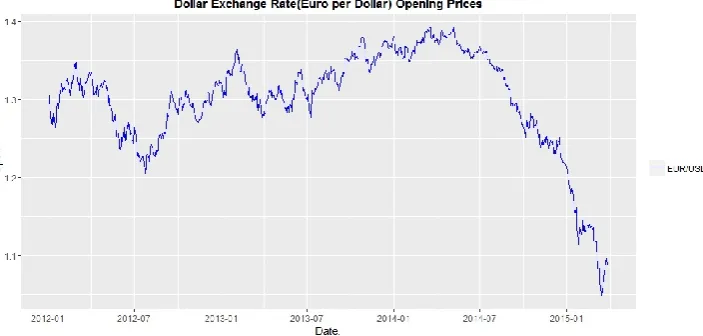
Hidden Markov Model that has been already proposed in the literature eliminates the risk of getting in both market directions, whether in bull or bear market. The main reason behind our decision to use EUR versus USD is that it is the most tradable pairs by traders. For that reason, it is a tradable quantity which makes our trading simulation more practical. The study examines the exchange rates from their first trading day since the end of January 2012.

II. LITERATURE REVIEW

Researching easy yet effective prediction techniques is a very difficult and complex task for foreign exchange rate practitioners. The conventional statistical methods seem to fail to capture discontinuities, the nonlinearities and the high complexity of datasets such as financial time series. Soft computing techniques like Hidden Markov Model (HMM) provide enough learning capacity and are more likely to capture the complex non-linear models which are dominant in the financial markets but their initial parameter is difficult to set. ((Hassan, 2009) and (Badge & Srivastava, 2010)). Despite of that, previous techniques let the trader have to identify the trend ((Bakhach, Tsang, & Ng, 2015) and make decision whether to buy or sell position (Oladimeji, 2016).

In contrast to previous studies, which focusing more on predicting the closing price, this study apply opening price to predict the price projection which is able to find the trader’s profitable entry point. The aim of this paper is to introduce a new application of Hidden Markov Model which is able to overcome the difficulties in setting the parameters of the model. For this purpose among the various Hidden Markov Model applications, we use the 3 input features consist of open, high, and low price value. These input values has been applied in (Hassan, 2009) which has proven experimentally to outperform the traditional Hidden Markov Model.

The mentioned three input variables has been applied in several studies including (Nath, 2005), (Kentucky & Emam, 2008), (Tiong, Ngo, Lee, & Bar, 2013). This methodology was applied for the prediction of the price of financial time-series. Despite the high prediction accuracy of the derived model, this methodology does not provide any method for analyzing the price projection from open price value. Moreover, the Hidden Markov Model to the task of forecasting financial series with ambiguous empirical evidence. (Ahani, Abass, & Okunoye, 2010) use the Hidden Markov Model to develop a simulation model of the Nigerian Stock Exchange using real life data collected from the daily stock market prices of the Nigerian Stock Exchange between the years 2005 and 2008 which assumed that the hidden states are bull, bear and Even. These hidden states, along with the observable sequences of large rise, small rise, no change, large drop and small drop, were used to develop the Hidden Markov Model. The visualization reveals that the stock exchange will only be steady periodically irrespective of initial conditions. The non -stationary and non-linearity of time series lead to an extension of the Hidden Markov Model to include a novel exponentially weighted Expectation-Maximization (EM) algorithm in (Zhang & Science, 2004) to handle these two challenges. This extension allows the HMM algorithm are proved using techniques from the EM Theorem. Experimental results show that their proposed model consistently beat the S&P 500 Index over five 400-day testing periods from 1994 to 2002, including both bull and bear markets.

The lowest BIC and AIC value is preferred. On the other hand the highest Log likelihood value is chosen for the best model.

Modelling high accuracy techniques for predicting time series is a very crucial problem for scientists and decision makers. The traditional statistical methods seem to fail to capture the discontinuities, the nonlinearities and the high complexity of datasets such as financial time series. Soft computing techniques like Hidden Markov Model provide enough learning capacity and are more likely to capture the complex non-linear models which are dominant in the financial markets but their initial parameter is difficult to set ((Hassan, 2009) , and (Badge & Srivastava, 2010)). (Bakhach et al., 2015) apply the Directional Change (DC) approach aims to capture directions price movements – whether to take a long or short position.

The main objective of this paper is to introduce a new application of Hidden Markov Model, which try to overcome some of these limitations. The proposed technique eliminates the number of parameters that the practitioner needs to experiment while on the other hand it increases the forecasting ability of the model.

Hidden Markov Model is employed in (Li & Cheng, 2015) to fit global, U.S. and European annual corporate default counts. All parameters are calibrated by using the Expectation-Maximization algorithm while the standard errors of the estimated parameters are conducted by Monte Carlo method. Little forecasting research has been done under the Directional Change (DC) framework motivates (Bakhach et al., 2015) to formulate a forecasting problem to answer the question of whether the current trend (up or down) will continue for a particular percentage (which is decided by the investor) before the trend ends. The trends movement also considered in (Komariah & Sin, 2015) for predicting the trends of USD Dollar/IDR Rupiah movement using Hidden Markov Model using the hidden variables correspond to people’s sentiment manifested by tweets every day. The study of financial time series trends continued by (Sandoval, 2015), which presents Hierarchical Hidden Markov Model used to capture the USD/COP market sentiment dynamics choosing from uptrend or downtrend latent regimes based on observed feature vector realizations calculated from transaction prices and wavelet-transformed order book volume dynamics. The new classification method for identifying up, down, and sideways trends in Forex market foreign exchange rates proposed by (Talebi, Hoang, & Gavrilova, 2014).

The performance of state-of-the-art machine learning techniques are investigated by (Theofilatos & Karathanasopoulos, 2012) in trading with the EUR/USD exchange rate using five supervised learning classification techniques (K-Nearest Neighbors algorithm, Naïve Bayesian Classifier, Artificial Neural Networks, Support Vector Machines and Random Forests). These techniques were applied in one day movement prediction of the EUR/USD exchange rate using autoregressive terms as inputs. The performance of the selected techniques was benchmarked with Naïve Strategy and moving average convergence/divergence model. The result shows that trading strategies produced by the machine learning techniques using Support Vector Machines and Random Forests outperformed all other strategies in terms of annualized return and sharp ratio. To the best of their knowledge, they came out with the first application of Random Forests in the problem of trading with the EUR/USD exchange rate providing extremely satisfactory results.

EUR/ALL exchange rate based on the patterns that previously occurred. EUR/ALL exchange rate on weekdays for a period of four years is used under study. Several experiments are conducted applying different parameters to both techniques. Root Mean Square Error (RMSE) is used as a measure to evaluate and compare the predictive power of SVM and ANN.

The EURJPY exchange direction is examined by (Haeri, Hatefi, & Rezaie, 2015) which attempt to forecast the price direction whether increase or decrease using five major indicators including exponential moving average (EMA), stochastic oscillator (KD), moving average convergence divergence (MACD), relative strength index (RSI) and Williams %R (WMS %R). Proposed approach is using hidden Markov models and CART classification algorithms is used for forecasting direction (increase or decrease) of Euro-Yen exchange rates in a day. Then the method is compared with CART and neural network. Comparison shows that the forecasting with proposed method has higher accuracy.

Generalized Autoregressive Conditional Heteroscedastic approach is considered in (Milano, 2013) to model the Eurodollar spot and futures exchange rate’s volatilities using daily and weekly observations, which apply different currency futures hedging strategies which minimize the foreign exchange risk in USD. (Ahmed & Straetmans, 2015) attempts to predict the cyclical behavior of exchange rates by using five risk factors, viz., violations of uncovered interest rate parity (UIP), relative purchasing power parity (RPPP) and pseudo-parity for equity returns, relative (cross-country) TED spreads and relative term spreads. These factors are found to forecast periods of depreciation or appreciation and subsequent reversals to form trading strategies and hedge their positions as well as re-balance their carry trade positions.

Compared to previous study, this paper avoids hedging strategy which is more risky to the trader’s portfolio. The proposed application also reduces the factors involves in making trading decisions and eradicate complex financial market trend calculations.

III.PROPOSED METHOD IN MODELLING THE EURO (EURO)/US DOLLAR (USD) EXCHANGE RATES

In this paper, the HMM has been applied to investigates the similar data pattern in exchange rates data that occur on a daily basis. Most time series analysis technique involves some form of identifying market trends. Hence, the traders need to decide whether they should buy, sell or hold the position. On the other hand, this study suggest the valuable risk based on daily price projection which the traders need to fill the buying and selling orders in each trading period. The HMM is proven as a powerful tool that work well for

sequential data modelling. Hidden Markov Model consists of a finite set of states, each of which is

associated with multidimensional probability distribution. Transitions among the states are governed by a

set of probabilities called transition probabilities. In a particular state an observation can be generated,

according to the associated probability distribution.

HMM contains following elements: i) N is Number of hidden states ii) Q is Set of states Q = {1,2,...,N} iii) M is Number of symbols

iv) V is Set of observation symbols V = {1,2,....,M} v) A is State Transition Probability Matrix

In order to implement HMM, the following three fundamental questions should be resolved

1. Given the model λ= (A, B, π) how do we compute P(O| λ), the probability of occurrence of the

observation sequence O = O1,O2, ….. , OT.

2. Given the observation sequence O and a model λ, how to choose a state sequence q1 , q2 , ….. , qT that

3. Given the observation sequence O and a space of models found by varying the model parameters A, B and π, how do we find the model that best explains the observed data.

The exchange rate data is published consists of the opening, closing, highest and lowest price for each time horizon including daily and hourly data. Based on mathematical expression has been researched by

(Badge, 2012), this study apply exchange rate prices on opening {oi}, highest {hi}, and lowest {li}for each

time horizon. The historical data has been used to predict the price range from the opening price to the highest price and from the opening price to the lowest price. The problem can be expressed as follows: n

pi+1 = ∏ f(oi, hi, li) (1)

i=1 where;

i = the stage in model on daily basis. In order to apply HMM, the historical data is divided into training and testing data set. Before applying Hidden Markov Model the main thing is to choose number of states and observation symbols. Given an observation sequence and the set of hidden states, we need to learn the Transition probability matrix {A} and the Observation probability matrix {B}, which are determined as follows:

A ={aij}s.t.aij = p[qt+1 = sj/qt=si] i ≤1, j ≤ N (2)

B ={bj(K)}s.t.bj(k) =p[vk =t/qt =sj] 1≤j≤N,1≤k≤M (3)

Where qt is the state at time t. Baum-Welch algorithm is used as a learning algorithm. The Baum-Welch

algorithm is a generalized expectation-maximization algorithm which to calculate maximum likelihood estimates and posterior mode estimates for the parameters of an HMM. The Baum-Welch algorithm searching for

λ= max p(O/ λ) (4)

which is the HMM λ that maximizes the probability of the observation O.

The application of the algorithm can be expressed as follows:

The forward probability and the backward probability has been calculated for each HMM state. The next stage is to find forward probability that can be expressed as αi(t) = p(O1=o1,,,Ot=ot, Qt=i| λ), that is the

probability of considering the partial sequence o1, , , ot and ending up in state i at time t. The calculation of

αi(t) as follows:

αi(t) = πibi(O1) (5)

N

αj(t + 1) = bj(Ot+1) ∑ αi(t).aij (6)

i=1

The backward probability is defined as the probability of the ending partial sequence Ot+1….OT given that

started at state i, at time t. The calculation of βi(t) as follows:

βi(T) = 1 (7)

N

βj(t) = ∑ βj(t + 1)aijbj(Ot+1) (8)

i=1

The Baum-Welch algorithm is used to find the similar patterns with the current day from the HMM

data pattern which assume that the produced likelihood value on day n is lpi. Based on the historical data

set using the HMM those observation sequences are located which would produce the same or nearly same

value of lpi. The HMM found the yth day’s observation sequences which would produce the same

likelihood value lopi. The price range variable on day ‘y’ and ‘y+1’ is determined.

pi+1 = (py+1 – py) + oi (9)

According to the above equation, py is the projection price of matched data pattern, py+1 equal to next day

projection price of matched data pattern and pi representing the projection price of today’s data.

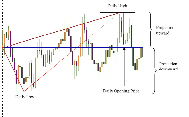
The HMM is trained to calculate the likelihood values of price range from the open price (Fig. 1) between two data sequences, in which past day price range behavior is first located which is almost similar to that of the current day. The range calculated produces the likelihood values for the current day, and then observation sequences are located which give nearly equal values which are formed from the past data sets. Then price difference of that day’s price and next to that day’s price are taken and hence next day’s price range is forecasted by adding the above difference to the current day’s opening price. In order to train HMM based tool is developed for time series forecasting, based on historical records of daily opening

price utilization as depicted in Fig.1. The prior probability πi, a random number has been chosen and

normalized;

1

1 



N

i i 

.

In this study, there are three input variables has been used in calculating the exchange rate price range. It consists of the opening, high and low price values of the day. The price projection calculated from the daily open price range which depicted in Fig.2 is the new method introduces in this study compares to previous researchers that concern more on the closing price of the day. The daily price range value as shown in Fig.3 which produced from the projection can be applied in risk and reward calculation in each trading period. In order to find the similar data patterns, the well known Baum-Welch algorithm is applied. The first step in training the parameters of an HMM is to see what states and transitions the model thinks are likely on each trading day. Those likely states and transitions can be used to reestimate the probabilities using the ‘forward-backward” or Baum-Welch algorithm, increasing the likelihood of the training data.

Fig. 2 Price Projection in two directions: upward and downward

Fig. 3 Price range between high and low of the day

Daily Opening Price

Projection upward

Projection downward

Daily Low

IV.EXPERIMENTAL RESULTS AND DISCUSSIONS

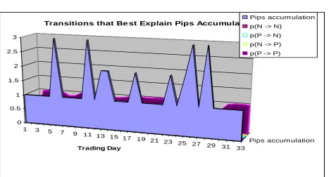
In order to train the HMM, the dataset is divided into two sets, one training set start from 4/1/2013 (3032 observations) and one test set begin at 29/7/2013 to 5/5/2016 (3574 observations). For example, the study compute the statistical parameters an HMM using the exchange rate of EUR/USD for the period 2/1/2012 to predict the range (TABLE 1) of price target 15/1/2012. The trained HMM and the past data, produced consistent 10 pips daily price range movement has been shown in Fig. 4 as pips gain, for the period 2 January 2012 to 15 January 2012. It can be stated that total pips accumulation for each trading period is greater than 0 which indicates that the probability of profitability is positive value. The Table 1 shows the similarities between two datasets (range of price movement 12 October 2011 and 20 May 2013 is 10 pips). It seems that 28 May 2013 price pattern repeated the price that of 2 January 2012.

TABLEI

DAILY DATA PATTERN FOR THE SPECIFIED TRADING PERIOD

Date Price

Range from the opening price

Open High Actual Predicted

12/10/2011 1.29234 1.29304 1.29304 1.29334

20/5/2013 1.29805 1.29915 1.29915 1.29905

Data pattern on 21/5/2013 that match data pattern on 12/10/2011 and 20/5/2013

1.25962 1.26242 1.26242 1.25972

1 3 _{5 7}

9 _{11 13 15 17}

19 21 23 _{25 27}

29 _{31 33} Pips accum ulation 0

0.5 1 1.5 2 2.5 3

Trading Day

Transitions that Be st Explain Pips Accumulation

Pips accum ulation p(N -> N)

p(P -> N) p(N -> P) p(P -> P)

The Table 2 shows that Model 1 and Model 2 produce the lowest AIC and BIC values compared to the

Model 3. The Model 3 produces the highest AIC and BIC values which cannot be considered as a

preferred model. In term of Log likelihood feature value as depicted in Table 3, Model 1 and Model 2 still

outperform the Model 3 with 9474.581. Model 3 fail to beat almost entirely the model parameter

comparisons, the trace left behind by the training set points, as a result making it the model with the poor

parameter estimation gain. The third model produces the lowest AIC and BIC with 18909.16 and

-18811.27 values compared to Model 1 and Model 3. It can be seen that in the AIC and BIC parameter

values, the first model produce the lowest value. Finally, it can be concluded that the Model 1 has proven

has the best parameter estimation compared to Model 2 and Model 3.

TABLE2

MODEL PARAMETER COMPARISON BASED ON AIC AND BIC VALUES

Model Difference AIC BIC

Model 1 Low and Open -19633.48 -19535.59

Model 2 High and Open -19678.55 -19580.65

Model 3 Close and Open -18909.16 -18811.27

TABLE3

MODEL PARAMETER COMPARISON BASED ON LOG LIKELIHOOD VALUE

V. CONCLUSIONS AND FUTURE WORK

This paper introduces the new approach of Hidden Markov model for financial forecasting purposes. The study applies the proposed technique to the task of forecasting the EUR/USD daily exchange rate which compared its result with 3 different models development. In terms of results, the selected technique outperforms all its benchmarks in terms of AIC, BIC, and Log likelihood value and trading efficiency for both in- and out-of-sample periods. The proposed technique produce consistent pips accumulation over the long run. Further improvements needs to be made on the proper selection of variables as inputs, more variables including technical and fundamentals factors. Future research could explore the possibility of coming up with a risk adjustment to produce easy and profitable trading strategy without burdening the

Model Difference Log likelihood

Model 1 Low and Open 9836.742

Model 2 High and Open 9859.273

traders with high risk and reward ratio. Recent research done on this field has shown the prospective return and applications that could be obtained for exchange rate forecasting by employing this easy predictive application. Future work could be to examine the impact of fundamental and technical variables, instead of price gaps, on the exchange rate price movement.

ACKNOWLEDGEMENT

The authors like to thank to all reviewers at Computer & Information Sciences, Universiti Teknologi PETRONAS, Perak, Malaysia who greatly helped us.

R

[1] Adebiyi, A. A., Adewumi, A. O., & Ayo, C. K. (2014). Comparison of ARIMA and Artificial Neural Networks Models for Stock Price Prediction, 2014, 9–11.

[2] Ahani, E., Abass, O., & Okunoye, O. B. (2010). Simulation of the Nigerian Stock Exchange Using Hidden Markov Model,

5(1), 29–41.

[3] Ahmed, J., & Straetmans, S. (2015). Predicting exchange rate cycles utilizing risk factors ☆. Journal of Empirical Finance, 34, 112–130. http://doi.org/10.1016/j.jempfin.2015.09.001

[4] Arumugam, P., & R, S. A. S. (2013). Stock Market Forecasting Using Hidden Markov Model with Clustering Algorithm,

3(May), 72–76.

[5] Badge, J. (2012). Forecasting of Indian Stock Market by Effective Macro- Economic Factors and Stochastic Model, 1(2), 39–51.

[6] Badge, J., & Srivastava, N. (2010). Future State Prediction of Stock Market Using, 5(1), 73–80.

[7] Bakhach, A., Tsang, E. P. K., & Ng, W. L. (2015). Forecasting Directional Changes in Financial Markets, 1–17.

[8] Can, C. E., Ergun, G., & Gokceoglu, C. (2014). Prediction of Earthquake Hazard by Hidden Markov Model ( around Bilecik , NW Turkey ), 6(3), 403–414. http://doi.org/10.2478/s13533-012-0180-1

[9] Christensen, R. H. B., & Pedersen, M. W. (2011). Chapter 6 - Model selection and checking.

[10] Haeri, A., Hatefi, S. M., & Rezaie, K. (2015). Forecasting about EURJPY exchange rate using hidden Markova model and CART classification algorithm, 4(1), 84–89. http://doi.org/10.14419/jacst.v4i1.4194

[11] Hassan, M. R. (2009). A combination of hidden Markov model and fuzzy model for stock market forecasting.

Neurocomputing, 72(16–18), 3439–3446. http://doi.org/10.1016/j.neucom.2008.09.029

[12] Hu, S. (1987). Akaike information criterion statistics. Mathematics and Computers in Simulation, 29(5), 452. http://doi.org/10.1016/0378-4754(87)90094-2

[13] Johnson, H. G. (1969). The Case For Flexible Exehange Rates , 1969 *, (March).

[14] Kentucky, W., & Emam, A. (2008). Optimal Artificial Neural Network Topology for Foreign Exchange Forecasting, (270), 63–68.

[15] Kevin, R., Emilie, P. C., Alain, L., & Denis, H. (2015). Achimer Hybrid hidden Markov model for marine environment monitoring, 8(1), 204–213.

[16] Komariah, K. S., & Sin, B. (2015). Hidden Markov Model Based Approach to USD Dollar / IDR Rupiah Currency Exchange Rate Prediction using Twitter Sentiment Analysis, 9–11.

[17] Lee, D. (2013). Trading USDCHF filtered by Gold dynamics via HMM coupling, 1–13.

[18] Li, L., & Cheng, J. (2015). Modeling and Forecasting Corporate Default Counts Using Hidden Markov Model, 3(5), 2–6. http://doi.org/10.7763/JOEBM.2015.V3.234

[19] Milano, P. D. I. (2013). Modeling the euro exchange rate using the, 0–104.

[20] Nath, B. (2005). Stock Market Forecasting Using Hidden Markov Model : A New Approach.

[21] Nguyen, N., & Nguyen, D. (2015). Hidden Markov Model for Stock Selection, (December 2014), 455–473. http://doi.org/10.3390/risks3040455

[22] Oladimeji, I. W. (2016). Forecasting Shares Trading Signals With Finite State Machine Variant, 3(4), 4488–4493. [23] Park, S. H., Lee, J. H., & Lee, H. C. (2011). Trend forecasting of financial time series using PIPs detection and

continuous HMM. Intelligent Data Analysis, 15(5), 779–799. http://doi.org/10.3233/IDA-2011-0495

[24] Sandoval, J. (2015). Computational Visual Analysis of the Order Book Dynamics for Creating High-Frequency Foreign Exchange Trading Strategies ., 51, 1593–1602. http://doi.org/10.1016/j.procs.2015.05.290

[26] Theofilatos, K., & Karathanasopoulos, A. (2012). Modeling and Trading the EUR / USD Exchange Rate Using Machine Learning Techniques, 2(5), 269–272.

[27] Tiong, L. C. O., Ngo, D. C. L., Lee, Y., & Bar, D. (2013). Stock Price Prediction Model using Candlestick Pattern Feature,

1(3), 58–64.

[28] Xhaja, D., Ktona, A., & Brahushi, G. (2014). Currency Exchange Rate Forecasting Using Machine Learning Techniques,

3(5), 1037–1041.